Optical Fiber Communications and Devicesan incorrectly Part 4 pot
Bạn đang xem bản rút gọn của tài liệu. Xem và tải ngay bản đầy đủ của tài liệu tại đây (1.14 MB, 25 trang )
Effects of Dispersion Fiber on CWDM Directly Modulated System Performance
65
will occur. At this length L
2
=C/(1+C
2
), C
1
becomes zero and the pulse becomes
unchirped. We define this situation as optimal.
Finally, with further propagation, the fast and the slow frequency components will tend to
separate in time from each other and pulse broadening will be observed.
On the other hand, the SPM alone leads to pulse chirping, with the sign of the SPM-induced
chirp being opposite to that induced by anomalous GVD.
In Figure 11, the leading edge of the pulse becomes red-shifted and the trailing edge of the
pulse becomes blue-shifted. If the effects of anomalous dispersion were present, with the
chirp induced by SPM some pulse narrowing would occur. This means that the effect of
SPM counteracts GVD.
Fig. 11. Input (left) and output (right) pulse shape and chirp.
The effect of GVD on the pulse propagation depends, mainly, on whether or not the pulse is
chirped, the laser injection pulse shape, [del Rio 2010], and also on the fiber SPM (Self Phase
Modulation [Hamza, M. Y., Tariq, S. & Chen, L. 2006, 2008]. With the correct relation
between the initial chirp and the GVD parameters, the pulse broadening (which occurs in
the absence of any initial chirp) will be preceded by a narrowing stage (pulse compression).
On the other hand, the SPM alone leads to a pulse chirping, with the sign of the SPM-
induced chirp, being opposite to that induced by anomalous GVD. This means that in the
presence of SPM, the GVD induced pulse-broadening will be reduced (in the case of
anomalous), while extra broadening occurs in the case of normal GVD.
4. Enhancing the performance of systems using negative and positive
dispersion fibers
In this section, we study that the transmission performance depends strongly on dispersion
fiber and DML output power. We demonstrated that systems using SMF fibers can achieve a
good performance if the DML output power is properly chosen. Finally, we have found a
mathematical expression that make an estimation for a power value to fix the laser power
output for each channel in WDM systems.
In order to study the CWDM system performance a simple arrangement is proposed, as can
be seen in Figure 12. We have selected 16 output channels with wavelengths , in agreement
Optical Fiber Communications and Devices
66
with Recommendation ITU-T G. 694.2. The pulse pattern was a periodic 128-bit OC-48 (2.5
Gb/s) nonreturn-to-zero (NRZ). After transmission through 100 km of fiber, channels are
demultiplexed and detected using a typical pin photodiode.
We have used two kinds of optical fibers; the already laid and widely deployed single-mode
ITU-T G.652 fiber (SMF) and the ITUT-T G.655 fiber with a negative dispersion sign around
C band (NZ-DSF). It is well known, SMF fiber dispersion coefficient is positive in the whole
telecommunication band from O-band to L-band and the dispersion coefficient of the NZ-
DSF fiber is negative in the optical frequency range considered. For our purpose, the same
spectral attenuation coefficient of both fibers has been considered whose water peak at 1.38
µm is well suppressed. The dispersion slope, effective area and nonlinear index of refraction
are compliant with typical conventional G.652 and G.655 fibers.
Fig. 12. Arrangement set up of simulated transmission link.
We have to point out that the transmission performance of waveforms produced by directly
modulated lasers in fibers with different signs of dispersion, depends strongly on the
characteristics of the laser frequency chirp. For this reason, we have modeled two DMLs
(made up of DFB-DMLs), by using the Laser Rate Equations in agreement with that reported
in [Tomkos 2001b], both DMLs presenting extreme behaviors [Hinton 1993]: DML-A is
strongly adiabatic chirp dominated; = 2.2 and k = 28.7 *10
12
(W.s)
-1
and DML-T is strongly
transient chirp dominated; = 5.6 and k = 1.5 *10
12
(W.s)
-1
. The and k values used in our
simulation are in agreement with potential commercial devices [Osinki 1987, Peral 1998,
Rodríguez 1995].
In this work, we are mainly interested in comparing the system performance based on the
type of fiber and DML used; for this reason, the rest of link components have been modeled
by considering ideal behavior.
The performance of transmission systems is often characterized by the bit error rate (BER),
which is required to be smaller than approximately 10
-12
for most installed systems.
Experimental characterization of such systems is not easy since the direct measurement of
BER takes considerable time at these low BER values. Another way of estimating the BER is
using the Q of the system, which can be more easily modeled than the BER.
The parameter Q , the signal-to-noise ratio at the decision circuit in voltage or current units,
is given by the expression[Alexandre 1997]
OM
OD
16
TX
TX
TX
RX
RX
RX
Optical
Fiber
1
1
2
2
16
Effects of Dispersion Fiber on CWDM Directly Modulated System Performance
67
10
10
II
Q
(13)
where I
i
and σ
i
are average values and variances of the “1” and “0” values for each pattern. Q
factor can be considered just a qualitative indicator of the actual BER and it can expressed as
1
2
2
Q
BER erfc
(14)
This parameter guarantee an error-free transmission of Q-Factor higher than 7,
corresponding to a BER lower than 10
–12
.
In order to study the transmission performance of DMLs presenting extreme behavior on a
fiber with positive or negative dispersion, a set of simulations were carried out; called Cases
A, B, C and D, as shown in Table 1. The quality of transmission between them has been
compared. Thus, Case-A deploys DML-A lasers and SMF fiber, Case-B: DML-A/NZ-DSF,
Case-C: DML-T/SMF and Case-D: DML-T/ DSF.
Case DML Optical Fiber
A DML-A SMF
B DML-A NZ-DSF
C DML-T SMF
D DML-T NZ-DSF
Table 1. Different configurations for the simulated system
The DML output power of all channels was varied from -10 dBm to 10 dBm (0.1-10 mw),
and the performance, in terms of Q-Factor, is analyzed for each transmitted channel.
Figure 13 shows the Q-Factor dependence on channel power for the wavelength channel
centered at 1551 nm.
Fig. 13. Simulated results for the transmission performance, Q-Factor, at 1551 nm
wavelength after transmission over 100 km of positive and negative dispersion fiber
Optical Fiber Communications and Devices
68
Independently of the Case and wavelength channels, the Q-Factor always presents a
maximum value for a specific DML output power [Horche 2008]. This behaviour
demonstrates the existence of an optimum channel power that will have to be considered
during the system design.
This optimum value corresponds with the power value that allows compensating the laser
chirp with the fiber dispersion and it depends on the combination of components used in
each case.
4.1 A and B cases: Adiabatic dominated laser
A and B Cases use adiabatic chirp dominated DML-A lasers. The Qmax value is reached at
0.3-0.46 mw, independently of the fiber type. Over this value the function drastically gets
worse when increasing the output laser power. In both cases the type of the laser used in the
simulation is an adiabatic chirp dominated, so for values over 0.4 mW the filter reduces
partially the spectrum and this phenomenon closes the eye diagram.
Fig. 14 shows the spectrum of adiabatic chirp dominated laser together with the transfer
function of a Gaussian filter. The shift of the spectrum towards blue would cause a bigger
reduction of the peak emission of bit “1” than the one produced on the peak of bit “0”. This
would bring both “1” and “0 peak emission power closer and the eye diagram be closed.
Fig. 14. Spectrum of adiabatic chirp dominated laser together with the transfer function of a
Gaussian filter
On the other hand, the power waveform coming from DML suffers a deformation when
getting through the dispersive media. In the case of DML-A, the result of the interplay of the
dispersion with the specific chirp characteristics will result in a high intensity spike at the
front of the pulses for transmission through a fiber with positive dispersion (SMF) and at the
end for negative dispersion (NZ-DSF) [Krehlik06], as can be seen at the top of the Figure 15.
The absolute value of the dispersion (and not its sign) will play a major role in the
transmission performance. Thus, the performance corresponding to transmission through
an SMF fiber will be worse than that corresponding to transmission through an NZ-DSF
fiber because of the larger absolute value of the dispersion.
Effects of Dispersion Fiber on CWDM Directly Modulated System Performance
69
Figure 15 represents the power waveforms for five different optical output powers (from 0.5
to 4 mw) after transmission through 100 km NZ-DSF fiber.
Fig. 15. Shapes of optical pulses for different DML-A output powers, after transmission
through 100 km negative dispersion fiber
The increment of P
ch
will result in a higher intensity spike at the trailing edge of the pulse.
As consequence the eye pattern after transmission will be severely closed.
In Fig. 16 the eye diagrams are shown for the case of the adiabatic chirp dominated
transmitter after transmission over 100 km of a negative dispersion fiber for (a) P
ch
= 0.46
mw (optimum power) and (b) P
ch
= 1 mw. For P
ch
= 0.46 mw, the eye pattern is clearly open,
while for P
ch
= 1 mw eye pattern experiencing more than 3dB eye closure.
a) P
ch
= 0.5 mw (b) P
ch
= 1 mw
Fig. 16. Eye diagrams for the case of the adiabatic chirp dominated transmitter after
transmission over 100 km of a negative dispersion fiber for (a) P
ch
= 0.46 mw and (b) P
ch
= 1
mw.
For small powers, the Q-Factor increases with P
ch
because a large amount of power reaches
the detector. For higher P
ch
the optical pulse deformation arising from chirp induced by
DML becomes too large and causes an error in pulse reconstruction.
Before transmission
After transmission
Optical Fiber Communications and Devices
70
4.2 C and D cases: Transient dominated laser
C and D Cases use transient chirp dominated DML-T lasers. For Case-C (DML-T/SMF), the
Q
max
value takes place for an output power of 6.7 mw approximately. In Case-D (DML-
T/DSF), the necessary output power to reach the Q
max
is around 2.3-3.4 mw.
In DML-T, the wavelength shift by laser transient chirp is a blue shift during the pulse rise
time and a red shift during the pulse fall time; exactly the opposite effects takes place with
SPM (Self-phase-modulation) [Suzuki 1993]. Therefore, the optical pulse chirped by direct
modulation is compressed in fibers with negative dispersion (NZ-DSF), while that chirped
by SPM is compressed in fibers with positive dispersion (SMF).
As it can be seen in Figure 13, for channel power Pch from 0.1 to 4 mw, the performance of
system that uses an NZ-DSF fiber (D-Case) is better than that of an SMF fiber (C-Case). In
this power range, SPM magnitude is not enough and the wavelength shift by laser transient
chirp is the predominant effect. Thus, the optical pulse chirped by direct modulation is
compressed in fibers with negative dispersion (NZ-DSF) and uncompressed in fibers with
positive dispersion (SMF). Therefore, case D is better than case C, however, for P
ch
. from 4
mw to 9 mw, Case-C (DML-T/SMF) presents a better performance than Case D (DML-
T/NZ-DSF) because of the increment in the magnitude of the SPM in the optical fiber and,
therefore, chromatic dispersion of the positive dispersion fiber is equalized by the SPM as
long as the pulses are broadened for negative dispersion fiber. As resulting from this, the
eye pattern after the transmission through SMF fiber will be more open than using NZ-DSF
fiber when higher output power is used.
Figure 17 shows the eye diagram of Case-C (a) and Case-D (b). In both cases a P
ch
. of 7 mw
was used and the eye diagram is measured for the signal transmission after 100 km of
dispersion fiber at 1551 nm wavelength. After the transmission through SMF, the eye look
perfectly open (Fig 17a) while the eye pattern after transmission through NZ-DSF is severely
closed (see Fig 17b) and intersymbol interference will occur. On other hand, the different
dispersion sign will only affect the asymmetry of the eye diagram, as is obvious from the
results of Fig. 17.
Therefore, we can conclude that systems using an SMF fiber can have a similar or better
performance to those systems that use an NZ-DSF fiber if the DML is transient chirp
dominated and its output power is properly chosen.
5. Management of the power channel of to enhance CWDM system
performance
In order to analyze the influence of the selected wavelength in a CWDM system, simulations
varying the number of channels from 1 to 16 have been carried out, using the same
schematic arrangement set up shown in Fig. 12. The channel wavelengths were between
1531 and 1591 nm. In this case, this wavelength range was used due to the system does not
need optical amplifiers. Some channels were located at compatibles frequencies with
CWDM ITU-T grid in order to, in the future, extend this work to whole useful fiber optic
spectral range (1271-1611 nm).
In every case, the Q-Factor shows a maximum value for a given optical output power. In A
and B Cases, due to small powers of channels, Q
max
is almost independent of number of
Effects of Dispersion Fiber on CWDM Directly Modulated System Performance
71
(a) Positive (b) Negative
Fig. 17. Eye diagram at the receiver side of a 2.5 Gb/s transient chirp dominated transmitter
(7 mw of output power at 1551 nm wavelength) over (a) SMF fiber where the dispersion is
positive and (b) NZ-DSF fiber where the dispersion is negative
channels. In C and D Cases, this maximum value decreases with the increment of the
number of channels used manly due to crosstalk between channels and others no-lineal
effects. However, the Q
max
value, for a given channel, takes place for a very similar output
power.
Figure 18 shows the Q-Factor versus channel power for channels centered at 1531, 1551, 1571
and 1591 nm respectively, for 16-Channel WDM system using DML-T/SMF (a) and DML-
T/DSF (b).
In both cases, each channel presents a different optimum P
ch
. Thus, by means of the P
ch
management of each channel it is possible to reach the Q
max
and enhances WDM system
performance can be achieving.
As an example; if a 16-Channel WDM system is designed using DML-T and SMF with
channel powers equal to the optimum channel power Pch. all 16 channels will have a Q
higher than 8, corresponding to a BER lower than 10
-15
. In contrast, if a system design with
equal channel power is used some of channels (higher dispersive channels) will fail after
propagation through SMF fiber.
In Case D, in order to guarantee a Q-Factor=15, the output power laser of the channels
centered at 1531, 1551, 1571 and 1591 nm should be 3.2, 3.5 3.8 4 mW respectively. Such
difference is due to the different fiber dispersion coefficients that would be associated to
every one of them, as shown in Table 2. Then, the compensation of the dispersion would
happen for different chirp values and therefore for different output power values.
From another point of view, if the system were designed with the same value of output
power in every laser, there is the risk for the channel with the bigger dispersion value not to
exceed the minimum criteria that assure an error-free transmission.
Optical Fiber Communications and Devices
72
(a) Case C (DML-T/SMF)
(b) Case D (DML-T/NZ-DSF)
Fig. 18. Q-Factor vs channel power for channels centered at 1531, 1551, 1571 and 1591 nm
respectively, for 16-Channel WDM system using DML-T/SMF (a) and DML-T/NZ-DSF (b).
Channel Dispersio
n
1531 nm 15,21 ps/nm·km
1551 nm 16,34 ps/nm·km
1571 nm 17,47 ps/nm·km
1591 nm 18,56 ps/nm·km
Table 2. Chromatic dispersion of differents channels (SMF fiber)
Since the optimum power channel depends on the global dispersion of the system, a study
including the variation of the accumulated dispersion of the global system will be done. The
optimum channel powers (P
ch
to reach Q
max
) are plotted as a function of dispersion in Fig. 19
(open circles in the case of transmission through positive dispersion fiber and solid circles
for negative dispersion fiber). In Fig. 19, the results for channel centered at 1551 nm after
transmission over 100 Km of SMF and NZ-DSF fibers as well as a potential CWDM channel
centered at 1391 nm are shown. Attenuation dependence with wavelength was taken
account in the calculation of optimum P
ch
and, in all cases, Q
max
higher than 7 (BER lower
than 10
-12
) was obtained.
Effects of Dispersion Fiber on CWDM Directly Modulated System Performance
73
Fig. 19. Comparison of Optimum Channel Powers versus accumulated dispersion for a
positive dispersion fiber (open circles) and negative dispersion fiber (solid circles).
In both cases, each channel presents a different optimum P
ch.
Then, by the P
ch
. control of
each channel it is possible to reach the Q
max
and an enhancement of the WDM system
performance can be achieved. This optimum P
ch
is the conclusion of the following
considerations: for low power levels, below the optimum power, the Q-Factor increases with
Pch because a larger amount of power reaches the detector and the performance
enhancement will be dependent upon the level power, so that the greater the power in the
receiver, higher system performance is obtained; while, for P
ch
higher than optimum power,
the chirp increases with level power and it causes greater frequency shift and linewidth
broadening which results in an error in pulse reconstruction.
A mathematical expression that fits this curve would be very useful, since it would make an
estimation of the power value to fix the laser output for each channel. For this reason, using
the Matlab simulation tool, this function has been estimated from a polynomial expression
of degree 4 (Figure 20)
Fig. 20. Estimated and approximated curve
Aproximated
Simulated
Optical Fiber Communications and Devices
74
432
()
f
xaxbxcxdxe
(15)
a = -3.482 ·10-14; b = -6.588·10-11; c = 4.202·10-07; d = 0.001435; e = 3.673
where x is the dispersion accumulated across the link.
Thanks to this equation it is possible to optimize the system behaviour reducing the number
of simulations needed for the design stage.
6. Conclusions
The performance of fibers relative to positive or negative dispersion characteristics is
discussed for the case of directly modulated lasers. The effects of chirp and fiber
nonlinearity in a directly modulated 2.5-Gb/s transmission system have been researched by
simulation. We have demonstrated that enhanced system performance, which uses a
positive dispersion fiber, can be achieved if positive chromatic dispersion in the optical fiber
is equalized by SPM, whereas laser transient chirp can be compensated using a negative
dispersion fiber. We can conclude that systems using SMF fiber can have a similar or better
performance to those systems that use NZ-DSF fiber if the DML is transient chirp
dominated and its output power is properly chosen.
Since the magnitude of SPM can be changed by controlling the optical power in the fiber,
the balance between SPM and laser transient chirp can be controlled. Therefore, an optimum
compensation condition can be achieved by controlling the optical DML output power. This
technique is simple, flexible, and applicable to WDM systems.
In order to analyze the effectiveness of this technique for WDM systems, simulations
varying the number of channels from 1 to 16 have been carried out and checking. In every
case, Q-Factor shows a maximum value depending on the optical power of each channel and
accumulated dispersion. This maximum value decreases depending on the number of
channels used. Also, we have shown that through the management of the Pch. of each
channel it will be possible to enhance the performance of each channel as well as the whole
WDM system.
7. Acknowledgements
The authors gratefully acknowledge the support of the MICINN (Spain) through project
TEC2010-18540 (ROADtoPON).
8. References
G.P. Agrawal (2010) Fiber-Optic Communication System. A John Wiley & Sons Ed.
S. B. Alexander (1997). Optical Communication Receiver Design. SPIE Press/ IEE.
J.C. Cartledge, G.S. Burley. (1989). The Effect of Laser Chirping on Ligthwave System
Performance. J. Lightwave Technol., vol. 7, no. 3, pp. 568-573.
L.A. Coldren and S.W. Corzine. (1995) Diode Lasers and Photonic Integrated Circuits. Wiley
Series in Microwave and optical Engineering.
Effects of Dispersion Fiber on CWDM Directly Modulated System Performance
75
C. del Río and P.R. Horche (2008). Directly modulated laser intrinsic parameters
Optimization for WDM Systems, International Conference on Advances in Electronics
and Micro-electronics, Sep-Oct 2008.
C. del Río, P. R. Horche, A. Martín Minguez (2010). Effects of Modulation Current Shape on
Laser Chirp of 2.5 Gb/s Directly Modulated DFB-Laser. Proceedings of The Third
International Conference on Advances in Circuits, Electronics and Micro-electronics.
CENICS 2010. ISBN.: 979-0-7695-4089-4
C. del Río, P.R. Horche, and A. M. Minguez (2010). Effects of Modulation Current Shape on
Laser Chirp of 2.5 Gb/s Directly Modulated DFB-Laser. Proc. Conf. on Advances in
Circuits and Micro-electronics, pp. 51-55, CENICS 2010
GVD effects in fiber optic communications: dispersion- and power-map cooptimization
using genetic algorithm, Optical Engg., volume 47, pp. 075003.
Hamza, M. Y., Tariq, S., Awais, M. M. & Yang, S. (2008). Mitigation of SPM and
Henry, C. H. (1982), Theory of the linewidth of semiconductor lasers, IEEE J.Quantum
Electron.,QE-18(2), 259–264.
K. Hinton and T. Stephens. (August 1993). Specifying Adiabatic Lasers for 2-5gbitls. High
Dispersion IM/DD Optical Systems. Electronics Letters. Vol. 29 No. 16.
P. Horche and Carmina del Río (2008). Enhanced Performance of WDM Systems using
Directly Modulated Lasers on Positive Dispersion Fibers. Optical Fiber Technology.
Volume 14, Issue 2, April 2008, Pages 102-108.
Krelik P. (2006)Characterization of semiconductor laser frequency chirp based on signal
distorsion in dispersive optical fiber". Opto-electronics review. vol. 14, no.2, pp. 123-128.
J.A. P. Morgado, and A.V. T. Cartaxo (October 2003). Directly Modulated Laser parameters
Optimization for Metropolitan Area Networks Utilizing Negative Dispersion
Fibers. IEEE Journal of Selected Topics in Quantum Electronics, Vol. 9, No. 5.
M. Osinski and J. Buss (January 1987). Linewidth broadening factor in semiconductor
lasers—An overview, IEEE J. Quantum Electron., vol. 23, no. 1, pp. 9–29,.
E. Peral, W. K. Marshall and A. Yariv (October 1998). Precise Measurement of
Semiconductor Laser Chirp Using Effect of Propagation in Dispersive Fiber and
Application to Simulation of Transmission Through Fiber Gratings. Journal of
Lightwave Technology, Vol. 16, No. 10,.
D. Rodríguez, I. Esquivias, S. Deubert, J. P. Reithmaier, A. Forchel, M. Krakowski, M.
Calligaro, and O. Parillaud. (February 2005 ). Gain, Index Variation, and
Linewidth-Enhancement Factor in 980-nm Quantum-Well and Quantum-Dot
Lasers. IEEE Journal of Quantum Electronics, Vol. 41, No. 2.
N. Suzuki, and T. Ozeki. (1993). Simultaneous Compensation of Laser Chirp, Kerr Effect,
and Dispersion in l0-Gb/s Long-Haul Transmission Systems. J. Lightwave Technol,
vol. 11, no. 9, pp. 1486-94.
Tomkos et. al. (2001a). Demonstration of negative dispersion fibers for DWDM metropolitan
Area networks, IEEE J. of Select. Top. in Quan. Elec. vol. 7, no. 3, pp. 439-60.
I. Tomkos, I. Roudas, R. Hesse, N. Antoniades, A. Boskovic, R. Vodhanel. (2001b). Extraction
of laser rate equations parameters for representative simulations of metropolitan-
area transmission systems and networks. Optics-Communications. 194(1-3): 109-29
I. Tomkos, R. Hesse, R. Vodhanel, and A. Boskovic. (March 2002). Metro Network Utilizing
10-Gb/s Directly Modulated Lasers and Negative Dispersion Fiber. IEEE Photon.
Technol. Lett., VOL. 14, NO. 3.
Optical Fiber Communications and Devices
76
L S. Yan, C. Yu, Y.Wang, T. Luo, L. Paraschis, Y. Shi, and A. E. Willner.(2005). 40-Gb/s
Transmission Over 25 km of Negative-Dispersion Fiber Using Asymmetric
Narrow-Band Filtering of a Commercial Directly Modulated DFB Laser. IEEE
Photon. Technol. Lett., vol. 17, no. 6, pp. 1322-1324.
4
Design and Application of X-Ray Lens in
the Form of Glass Capillary Filled by a
Set of Concave Epoxy Microlenses
Yury Dudchik
Institute of Applied Physics Problems
of Belarus State University
Belarus
1. Introduction
Glass capillaries are widely used in X- optics. It is a well know fact that a simple glass
capillary acts as a waveguide for X-rays because refractive index for X-rays in any medium
is less than unity. X-rays transmit glass capillary in the regime of total external reflection
instead of visual light that propagates inside glass fiber in the regime of total internal
reflection. X-rays also may transmit curved capillaries and, as was proposed by Kumakhov,
a bunch of curved capillaries act as a lens that focuses X-rays from a point source into a focal
point. This device is known as Kumakhov X-ray lens (Kumakhov & Sharov, 1992). Another
well-known X-ray device is a taper or parabolic single capillary that is used to condense or
focus synchrotron X-rays into micron-sized spot (Thiel et al., 1992).
Recently a new application of glass capillaries for X-ray optics was proposed: it was
demonstrated that capillaries are suitable for designing so named compound refractive X-
ray lenses.
Compound refractive X-ray lens at the first time was proposed by A. Snigirev, V. Kohn, I.
Snigireva and B. Lengeler (Snigirev et al., 1996) and their idea is based on the following
principles. It is a well-known fact that refractive lens for X-rays should be concave instead of
convex for visual light. Calculation shown that the focal length F
1
of such biconcave
spherical lens is determined by the following ratio:
F
1
= R /(2
), (1)
where R-radius of the lens and (1
) is real part of refractive index n. The focal length of the
lens is rather large (5-10 m for 5-8 keV X-rays) even when the curvature radius of the lens is
equal to hundred of micrometers. The large value of the lens focal length was a reason of the
conclusion that there is no any practical interest to focus X-rays by refractive lens. Attempts
to reduce focal length of the lens have resulted in creation of a compound refractive lens
(CRL) for X-rays with energy 5-30 keV (Snigirev et al., 1996). The lens consists of a large
number (10-300) of biconcave lenses, made of material with a low-atomic weight (beryllium,
carbon, polymers, aluminium). Focal length F of such lens is defined by the following ratio:
F= F
1
/ N , where N- is the number of lenses. The equation for F shows that the focal length
Optical Fiber Communications and Devices
78
of a compound lens can reach value of 1 m at R=0.5 mm. That is quite acceptable for
practical applications.
At present compound X-ray lenses are designed by some ways: by using pressing technique
for individual lens, by lithographic method, by drilling holes in a plate by a laser (Lengeler
et al., 2005). The problem of the lens design is how to produce individual concave lens with
a high quality parabolic or spherical shape surface and with curvature radius up to 50
microns or less. Another problem is to stack the lenses coaxially to form compound lens.
The idea of compound X-ray lens was advanced in our work (Dudchik & Kolchevsky, 1999),
where it was realised in the form of glass capillary filled by a large number of epoxy drops.
The lenses were designed at the Institute of Applied Physics Problems of Belarus State
University. The lens was named as microcapillary one and applied at synchrotron SPring-8
for focusing of 18 keV X-rays and as an objective of X- ray microscope
(Kohmura et al.,
1999). The lens consists of a glass microcapillary, filled by a plenty of biconcave microlenses.
The concave microlenses inside the capillary were formed by putting air bubbles into epoxy.
The schematic view of the lens is shown in Fig. 1.
d
1 2 3 4
2R
2R
d
1
F
Fig. 1. Schematic view of the microcapillary X-ray lens. 1- X-ray beam; 2- diaphragm; 3-
capillary; 4- epoxy lens
It was shown
(Dudchik et al., 2000) that the microlenses inside the capillary are spherical
ones and its curvature radius is equal to capillary one. This founded dependence of the lens
curvature radius on the capillary one leaves a room to decrease the lens focal length. For
example the lens in the form of 200 microns in diameter capillary and filled by 103
microlenses has 13-cm focal length for 8 keV X-rays. It was shown experimentally by
Adelphi Technology, Inc. using beamline 2-3 at the Stanford Synchrotron Radiation
Laboratory (SSRL) (Dudchik et al., 2004). Such short-focal-length lenses are suitable for
imaging not only with synchrotron X-rays, but with X-rays from laboratory sources of
radiation (Piestrup et al., 2005).
The purpose of the paper is to consider details of microcapillary lens design as the lens
application for focusing and imaging of X-rays.
2. Design and application of microcaplillary X-ray lens
2.1 Fabrication technique for the microcapillary refractive X-ray lens
The method of the microcapillary lens preparation consists (Dudchik & Kolchevsky, 1999;
Dudchik et al., 2000) in consecutive producing of air bubbles inside of capillary 1, filled by
epoxy 2 with using of capillary 4, connected with a cylinder with compressed air 5, as is
Design and Application of X-Ray Lens in the Form of
Glass Capillary Filled by a Set of Concave Epoxy Microlenses
79
shown in Fig.2. The growth of the bubble inside of the capillary 1 is supervised by visual
light microscope. When the radius of the bubble is becoming equal to the radius of the
capillary 1, the capillary 4 is moving to a distance of few microns from the received bubble
and the process is repeated. The liquid between two bubbles has a form of biconcave lens.
This technique actually has not restrictions in number of lenses. The photo of epoxy lenses,
made by the method, is shown in Fig. 3. The diameter of the capillary is equal to 0.2 mm (a)
and 0.8 mm (b).The air bubbles between lenses are observed as black ones. Used epoxy
consists of carbon, oxygen, hydrogen and nitrogen which are chemically bonded in
proportion C
200
H
100
O
20
N. The epoxy density is 1.08 g/cc.
1
2
3 4 5
Fig. 2. Schematic view of the setup for microcapillary X-ray lens fabrication. 1- glass
capillary tube; 2- glue; 3-air bubbles; 4- injector needle; 5- cylinder with a compressed air
Fig. 3. Visible light microscope image of the microcapillary refractive X-ray lens. The
diameter of the capillary is equal to 0.2 mm (a) and 0.8 mm (b).
Important parameter of the lens is thickness d (Fig.1), which for the given material of the
lens depends on the diameter of the capillary channel and on the epoxy temperature. We
established that for the lens made from epoxy, the lens thickness d might be decreased up to
5-10 microns.
The shape of the lens surface was investigated by an optical method with the help of optical
microscope connected with digital camera. The obtained individual lens image was
processed by computer. In Fig. 4 (a, b) the images of two lenses are shown. The curve,
dividing a light and a dark parts in Fig. 4 was considered as a profile of the lens. At
construction of the lens profile we took into account, that the visible lens diameter 2R is
more than the real diameter of the channel 2R
real
(Fig. 5).
We took into account that the light, that scatters from the inner wall of the lens, does not
come directly to the microscope. It is doubly refracted at the (lens-material)-glass and glass-
air boundaries. This is a reason why the observed lens profile differs from the real one.
Optical Fiber Communications and Devices
80
a)
b)
Fig. 4. Visible light microscope images of concave epoxy lenses inside capillary. a) Capillary
radius is equal to 0.39 mm; b) capillary radius is equal to 0.21 mm
Formulas for calculating lens profile can be found from a geometrical paths of rays, forming
the image of the lens (Fig. 5.). According to the Snell’s law:
n
lens
sin
= n
glass
sin
; n
glass
sin
= sin
, (2)
where n
glass
is the index of refraction of the glass, n
lens
is the index of refraction of the lens
material, sin
=R
/ ( n
lens
R
chan
), sin
=R
/ ( n
glass
R
chan
), sin
=R/ ( n
glass
R
cap
), sin
=R
/ R
cap
.
2Rreal
2Rcap
2Rchan
glass capillar
y
e
p
ox
y
g
lu
e
Rcap
Rrea
l
glass
epoxy glue
2R
Rchan
Fig. 5. Schematic view of the transverse section of the microcapillary lens. The rays of visible light
forming lens image also are shown. Rcap- is the outer radius of the capillary; Rchan- is the radius
of the capillary channel; Rreal- is the measured value of the profile; R- visible value of Rreal.
Design and Application of X-Ray Lens in the Form of
Glass Capillary Filled by a Set of Concave Epoxy Microlenses
81
From eq.(2) the radius of the channel, shown in fig. 4 as R
real
, is equal to:
R
real
=R/ (n
lens
cos (
+
-
-
) ). (3)
The obtained formula for R
real
was used for calculation of the lens profile. Fig. 6 shows the
profile of lens in comparison to the circle, radius of which is equal to the radius of the
capillary. As it can be seen from Fig. 6, the form of the microcapillary lens can be accepted as
spherical one, and the radius of lens curvature R is equal to the channel radius R.
This result is in a good agreement with classical molecular theory. The theory states that the
form of liquid drop putt into microcapillary can be accepted as biconcave spherical, and the
radius of drop curvature is connected by the following ratio to the capillary radius R
chan
:
R=R
chan
/ cos , (4)
where - angle of contact. For epoxy glue located on a glass surface, angle of contact is equal
to 0
0
.
-200 -150 -100 -50 0 50 100 150 200
0
20
40
60
80
100
120
140
160
180
200
microns
circle
microns
measured dat a
a)
-300 -200 -100 0 100 200 300
50
100
150
200
250
300
350
400
m
i
crons
circle
microns
measured data
b)
Fig. 6. Measuered profiles of the lenses. a) Capillary radius is 210 microns; b- capillary
radius is 390 microns
2.2 Parameters of the microcapillary refractive lens
Lens focal length f of compound refractive X-ray lens is calculated as (Snigirev et al., 1996):
2
R
f
N
, (5)
where R- curvature radius, N- number of microlenses, (1
)- real part of refractive index for
X-rays. Parameter
for used epoxy may be calculated from the epoxy chemical formula as
2
22
0.5
E
, (6)
where E is photon energy measured in eV. Experiments on measuring lens focal length of
compound epoxy lenses at Stanford Synchrotron Radiation Laboratory and at Advanced
Optical Fiber Communications and Devices
82
Photon Source by Adelphi Technology, Inc. shown validity of formula 6 for calculation lens
focal length (Dudchik et al., 2004).
Compound X-ray lens consisting of spherical microlenses may be characterized by
absorption aperture radius R
a
that in a good approximation can be calculated as (Snigirev et
al., 1996; Dudchik et al., 2004; Piestrup et al., 2005):
1
2
2
a
R
R
N
, (7)
where
is the linear absorption coefficient for the lens material.
The discussed X-ray lens is a linear combination of spherical microlenses and spherical
aberrations occur just in the same way as for spherical visual-light lens. To take into account
this phenomenon at least two planes around the lens focus may be denoted: they are shown
by the lines MS and PP in Fig.7 which shows trajectories of 8-keV X-rays forming focal spot
of compound lens consisting of 103-microlenses.
The plane PP represents a focal plane. The plane MS represent the circle of the least
confusion (Born @ Wolf, 1975). For spherical lens the size of X-ray beam at MS and PP
planes may be decreased by using diaphragm. The beam radius R
pp
at the PP-plane depends
on the radius of used diaphragm R
d
and is calculated from the third order aberration theory
as (Born @ Wolf, 1975):
3
pp
d
RfBR (8)
where f is the lens focal length, B is Seidel coefficient, R
d
is radius of the diaphragm placed
before the lens. Eq. 8 is valid for the case of the point source located at the infinity. As it
was shown in (Dudchik et al., 2000), the equation (8) for compound X-ray lens is rewritten
as
3
2
1
2
d
pp
R
R
R
. (9)
The eq. 9 is valid for the case when R
d
< 0.6 R as was estimated in (Dudchik et al., 2000) by
numerical calculations. The beam radius R
ms
at the MS-plane is related to the beam radius
R
pp
at the focal plane as
3
2
11
48
d
ms pp
R
RR
R
. (10)
The distance L
ms
from the lens to MS-plane is calculated as:
dms
ms
d
pp
RR
Lf
RR
. (11)
For example L
ms
= 0.917 f when R
d
= 0.5 R and it is illustrated by Fig. 7 where position of MS-
plane is shown for the discussed case.
Design and Application of X-Ray Lens in the Form of
Glass Capillary Filled by a Set of Concave Epoxy Microlenses
83
Fig. 7. Paths of 8-keV X-rays forming focal spot of 103- elements lens. Lens radius is 100
microns. Diameter of the diaphragm placed before the lens is equals to 100 microns
Radius R
ms
of the circle of the least confusion decreases with decreasing of the size of
diaphragm and achieves its minimum possible value R
ms- min
when a diaphragm with an
optimal hole radius R
d-opt
is used. In this case the value R
ms- min
will be equals to the radius of
the first minimum of the Airy diffraction pattern R
diff
which is R
diff
= 0.61
L
ms
/ R
d-opt
. The
diaphragm radius R
d-opt
may be defined by the following equation:
3
2
0.61
1
8
dopt
ms
do
p
t
R
L
R
R
(12)
where
is the wavelength. The solution of the Eq. (12) for R
d-opt
and for R
ms- min
under the
assumption L
ms
=f is:
1
3
4
2.44
dopt
R
R
N
, (13)
and
min
0.61
ms
do
p
t
f
R
R
. (14)
It is interesting to compare above result for R
d-opt
(Eq. 13) with the value of so-named
parabolic aperture radius R
p
. Parabolic aperture radius R
p
is the central portion of the
spherical lens that focuses X-rays to the same point. From wave approximation it is known
(Snigirev et al., 1996; Piestrup et al., 2005) that the value may be calculated as:
1
3
4
2
p
R
R
N
. (15)
Optical Fiber Communications and Devices
84
Comparing Eq.13 and Eq.15 we can see that there is only a small deference in numerical
coefficient for these two values. It may be explained that we used f value instead of L
ms
when
solving Eq.12.
Eq. (13) for R
d-opt
and Eq. (12) for R
ms- min
are useful to calculated expected X-ray beam size in
the MS plane for compound X-ray lenses. In Table 1 and Table 2 the diameter 2R
ms
of the
circle of the least confusion is calculated for epoxy spherical lenses with deferent values of
number of microlenses N and lens radius R. Table 2 shows result of the same calculations for
the case when additional diaphragm is used to decrease size of the beam at MS plane.
From the Table 2 it is seen that spherical compound refractive lens being combined with
diaphragm ensures resolution at submicron level.
Lens parameters Lens focal
length f for 8
keV X-rays, mm
Lens
absorption
aperture 2Ra,
µm
Lms value for
8 keV X-rays
beam , mm
Diameter (2R
ms
)
of the circle of
the least
confusion, µm
N=100, R=100 µm 132 117 117.5 5
N=200, R=100 µm 66 82 62 1.72
N=100, R=50 µm 66 82 53.5 6.89
N=200, R=50 µm 33 58 29.4 2.44
Table 1. Parameters of X-ray beam formed by spherical compound epoxy X-ray lens.
Lens parameters Lens focal
length f for 8
keV X-rays, mm
Diameter of the
optimal
diaphragm
aperture 2Ropt,
µm
Lms value for 8
keV X-ray
beam , mm
Diameter 2R
ms
of the circle of
the least
confusion, µm
N=100, R=100 µm 132 62 127.4 0.78
N=200, R=100 µm 66 53.2 64.3 0.46
N=100, R=50 µm 66 37.6 62.7 0.66
N=200, R=50 µm 33 31.6 31.8 0.39
Table 2. Parameters of X-ray beam formed by spherical compound X-ray lens combined
with diaphragm.
2.3 Measurement of the microcapillary refractive lens at Stanford Synchrotron
Radiation Laboratory
Refractive X-ray lens work as ordinary lens for visual light and lens formula is also valid to
describe its operation. The formula is written as:
11 1
ab f
, (16)
Design and Application of X-Ray Lens in the Form of
Glass Capillary Filled by a Set of Concave Epoxy Microlenses
85
where a is distance from the source to lens, b
is distance from the lens to source image, f -
lens focal length. The size of the source image S
1
, as in the case of visual optics, is related to
the source size S by the equation:
1
f
SS
af
. (17)
In the case of synchrotron radiation the distance between the source and the lens is high
enough and equals, as a rule, to 10-50 m; the size of the source is also, as a rule, less than
1000 microns. When refractive lens with a focal length equal to approximately 10 cm is used,
expected size of source image may be equal to some microns in according to formula 17.
This is a way for obtaining micro and nano-sized X-ray beams.
We fabricated and tested some microcapillary refractive X-ray lenses for focusing
synchrotron X-rays. The lenses were arbitrarily designated as 1-1, 3-1, 3-4, 3-3, 4-1 and 5-1.
The calculated and measured characteristics of these CRLs are given in Table 3 below.
X-ray lens designation 1-1 3-1 3-4 3-3 4-1 4-1
Photon energy, keV 12 12 9 8 8 7
Number of individual lenses 90 196 103 93 102 102
Lens curvature radius, m
165 250 100 100 100 100
Calculated focal length, cm 52.8 37 15.7 13.8 12.6 9.6
Calculated image distance, cm 54.5 37.8 15.8 13.9 12.6 9.7
Measured image distance, cm 32 36 17.5 13 14 10
Calculated vertical minimum waist diameter, m
15.1 10.4 4.4 3.9 3.2 2.7
Measured vertical minimum waist diameter, m
12.8 12 3.9 4.8 2.7 4
Calculated horizontal minimum waist diameter, m
64.1 44.0 18.8 16.6 13.5 11.5
Measured peak transmission, % 36 30 24 16 27 5
Calculated attenuation aperture diameter, m
314 262 143 125 119 96.7
Measured attenuation aperture diameter, m
321 245 147 150 149 149
Calculated 2D-gain 16.6 20.0 25.6 16.9 28.9 6.0
Measured 2D-gain 8.9 3.5 13.4 ** 25.5 **
Table 3. Measured and calculated parameters of microcapillary refractive X-ray lens for
SSRL BL 2-3 source
Used was the beamline 2-3 on the Stanford Synchrotron Radiation Laboratory’s (SSRL’s)
synchrotron (Dudchik et al., 2004). This beamline possesses a double-crystal
monochromator that was capable of giving x-rays from 2400 to 30000 eV with a 5 x 10
-4
resolution. The approximate source size (full width half maximum, FWHM) was 0.44 x 1.7
mm
2
, as specified by SSRL. The experimental apparatus is shown in Fig. 8.
The distance from the source to lens was 16.81 meters. The X-ray beam size from this source
was approximately 2 x 20 mm
2
at the entrance to the experimental
station; however, this size
Optical Fiber Communications and Devices
86
Fig. 8. The experimental apparatus at SSRL for measuring microcapillary X-ray lens
was reduced to approximately 0.4 x 0.4 mm
2
by Ta slits upstream of the monochromator.
The CRL was placed in a goniometer head that could be manually tilted in three axes. The
lens could also be remotely translated orthogonally (x and y) to the direction of the x-ray
beam to maximize the x-ray transmission though the lens. An x-ray gas ionization detector
was placed after a translatable slit for measuring the x-ray beam profile. This Ta slit was
adjusted to below 25 m by using a thin stainless steel shim. It is likely that, as good as the
Ta slit was, the jaws are not ideally parallel at these small dimensions, and the slit width
was minimally > 3 m when jaws appeared to be entirely closed.
After the slit width was adjusted, the Ta slit was then translated in the x direction across the
focused x-ray beam, and its profile obtained. We then manually moved the slits along the z-
axis of the x-ray beam, measuring its vertical widths by scanning the slits in the x direction
across the beam at each location.
Using these measured widths, we profiled the beam waist as a function of distance from the
lens. Results are shown in Table 3. For example, the source of diameter 0.44 mm was
focused by the lens 4-1 to a minimum spot FWHM of 5 microns, at a distances of 13 cm from
the CRL. Thus, the demagnification was M = .0114. The spot size in the horizontal direction
was measured to be 19 microns, which is larger, because the imaged source diameter was
larger (1.7 mm, FWHM) in that dimension.
The CRL has an aperture with a Gaussian absorption profile, which causes stronger
absorption of the extreme rays passing through the CRL outer radial regions, as compared
to rays that pass through the less absorptive central region. The CRL aperture is much
smaller than the source size, especially in the horizontal dimension. We obtained the
transmission through the CRLs given in Table 3 by narrowing the x-ray beam to 50 x 50 µm
2
and translating each CRL through the beam, thereby producing transmission profiles of the
lenses. The absorption apertures (e
-2
points, not FWHMs) were obtained from these figures.
The calculated and measured peak transmissions (transmission at the lens axis) for the
lenses are given in Table 3.
Given the measured transmissions and profiles, we determined the gains of these lenses.
Both measured and calculated gains are given in Table 3 for all these lenses. The gain
values varied between 3.5 to 25.5. These gain values are primarily due to the large source
size. If the same lens is placed on a beam line using a third generation X-ray source, the
gain of the CRL can be substantially larger. These sources can possess spot sizes a factor
Design and Application of X-Ray Lens in the Form of
Glass Capillary Filled by a Set of Concave Epoxy Microlenses
87
of 3 smaller (e.g. 0.5 by 0.5 mm
2
). Also, typical distances from insertion devices to end
stations can be approximately 51 m, as compared to 16.8 m in our experiment. For these
source parameters, the gain at 11 keV from the same lens is 138, a sizable increase of the
intensity over that of the case without a CRL. Although the gains of these CRLs were
small, larger gains can be achieved using smaller source sizes, larger CRL apertures, and
longer object distances.
2.4 Measurement of the microcapillary refractive lens at ANKA Synchrotron Radiation
Source
Parameters of the lens # 5-1 were measured at ANKA Synchrotron Source (Germany)
(Dudchik et al., 2007a). The lens was designed in Institute of Applied Physics Problems of
Belarus State University. The lens consists of 224 spherical epoxy microlenses formed inside
glass capillary with curvature radius equal to 100 microns. Lens length is equal to 69 mm.
The individual epoxy lenses inside of the glass capillary are spherical ones with the
curvature radius equals to 100 microns. Spherical lenses may be characterized by the
following set of parameters: lens focal length f, absorption aperture radius R
a
(see formula 7),
parabolic aperture radius R
p
( see formula 15) , and the diffraction radius R
diff.
=0.61
f/R
a
,
that characterises diffraction blurring of the focused beam, where
is linear absorption
coefficient for the lens material.
The lens # 5-1 was used to focus X-rays with energy 12 keV and 14 keV. Calculations show
that for 12 keV X-rays parabolic aperture radius of the lens is R
p
=27 microns for the case of
the discussed lens (R= 100 microns, N= 224). The absorption lens aperture radius Ra for the
lens is equal to 69 microns. The same values for 14 keV X-rays are : R
p
=28 microns, R
a
=94
microns. Lens focal length f calculated by formula 5 for 12 keV and 14 keV is equal to 133
mm and 180 mm respectively. The lens length is equal to 69 mm and it is “thick enough”
comparing to lens focal length. The focal length f
t
of a thick lens may be calculated by the
next formula (Pantell et al., 2003):
1/2
1/2
sin
t
t
f
f
f
t
f
, (18)
where t is lens length. Result of calculation of f
t
: f
t
= 145 mm for 12 keV X-rays and f
t
= 192
mm for 14 keV X-rays.
The lens #5-1 has been characterized for 12 keV and 14 keV X-rays at the ANKA-FLUO
experimental station situated at a bending magnet of the ANKA Synchrotron Light Source.
The energy was monochromatized by a W/BC4 double multilayer monochromator with 2%
bandwidth. For the measurement of the beamsize the lens was placed on a five axis
positioning device and exactly oriented in the direction of the X-ray beam. The distance a
between source and lens was equal to 12.7 m. The size of the source s: 800x250 µm
2
FWHM.
The source size can be reduced by a 0.1mm x 0.1 mm
2
slit #1 placed at a distance 4.7 m to the
source. There was one more slit #2 placed at 1m distance from lens. The slit size was 0.1mm
x 0.08 mm
2
. It was also possible to hold slits in opening mode.
Optical Fiber Communications and Devices
88
Measured were beam size at different distance to the lens and lens transmission. The
minimum value of beam size was considered as lens image distance. The beam size was
derivated from knife edge scans conducted around the focus position derived with the x-ray
camera. A 0.5 µm thin Permalloy structure was chosen and the edges have been scanned
with 0.5 µm or 1 µm resolution. Characteristic K
Fe-atom X-rays emitted by Permalloy
structure were registered by X-ray camera. The measured profile of the edge is the
convolution of the Fe concentration function (approximated by a step function) and the
profile of the x-ray beam. As the step function converts the convolution in to a simple
integration, the measured function is the error function if the beam profile is a Gaussian.
Thus an error function (Fig. 9) has been fitted to the knife edge data. Fitting a Gauss function
to the derivative is equivalent; nevertheless numerical derivating adds a considerable
amount of noise to the data.
a)
b)
Fig. 9. Fit of error function to vertical (a) and horizontal (b) scan over lithographic structure
To determine gain in intensity of the beam due to focusing by the lens next procedure was
applied. The lens was removed and the fluorescence intensity resulting from a Permalloy
square of 50µm size was measured. This intensity was compared to the intensity of the
focussed beam and the area of the focussed beam was calculated with A=2
x
y
with being
the Gaussian beamsize (FWHM value/2.35). With closed front end slits the gain factor for a
smaller source can be obtained. For the ANKA source however closing slits cannot improve
the gain. Therefore two values for the gain are given in Table 4 and Table 5.
Investigations shown that tested lens is suitable to focus 12 keV-14 keV X-rays into some
microns in size spots (Dudchik et al., 2007a). Calculated lens focal length is in a good
agreement with measured one. The lens parameters may be improved my increasing lens
transparency. Also lenses with shorter lens focal length may be formed inside capillary
with inner diameter equals to 100 microns. In this case the lenses may be used for nano-
focusing.