Báo cáo hóa học: " Research Article Some Shannon-McMillan Approximation Theorems for Markov Chain Field on the Generalized Bethe Tree" docx
Bạn đang xem bản rút gọn của tài liệu. Xem và tải ngay bản đầy đủ của tài liệu tại đây (566.8 KB, 18 trang )
Hindawi Publishing Corporation
Journal of Inequalities and Applications
Volume 2011, Article ID 470910, 18 pages
doi:10.1155/2011/470910
Research Article
Some Shannon-McMillan Approximation
Theorems for Markov Chain Field on the
Generalized Bethe Tree
Kangkang Wang
1
and Decai Zong
2
1
School of Mathematics and Physics, Jiangsu University of Science and Technology,
Zhenjiang 212003, China
2
College of Computer Science and Engineering, Changshu Institute of Technology,
Changshu 215500, China
Correspondence should be addressed to Wang Kangkang,
Received 26 September 2010; Accepted 7 January 2011
Academic Editor: J
´
ozef Bana
´
s
Copyright q 2011 W. Kangkang and D. Zong. This is an open access article distributed under
the Creative Commons Attribution License, which permits unrestricted use, distribution, and
reproduction in any medium, provided the original work is properly cited.
A class of small-deviation theorems for the relative entropy densities of arbitrary random field on
the generalized Bethe tree are discussed by comparing the arbitrary measure μ with the Markov
measure μ
Q
on the generalized Bethe tree. As corollaries, some Shannon-Mcmillan theorems for
the arbitrary random field on the generalized Bethe tree, Markov chain field on the generalized
Bethe tree are obtained.
1. Introduction and Lemma
Let T be a tree which is infinite, connected and contains no circuits. Given any two vertices
x
/
y ∈ T, there exists a unique path x x
1
,x
2
, ,x
m
y from x to y with x
1
,x
2
, ,x
m
distinct. The distance between x and y is defined to m − 1, the number of edges in the path
connecting x and y. To index the vertices on T, we first assign a vertex as the “root” and label
it as O. A vertex is said to be on the nth level if the path linking it to the root has n edges. The
root O is also said to be on the 0th level.
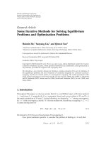
Definition 1.1. Let T be a tree w ith root O,andlet{N
n
,n ≥ 1} be a sequence of positive
integers. T is said to be a generalized Bethe tree or a generalized Cayley tree if each vertex
on the nth level has N
n1
branches to the n 1th level. For example, when N
1
N 1 ≥ 2
and N
n
N n ≥ 2 , T is rooted Bethe tree T
B,N
on which each vertex has N 1 neighboring
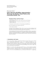
2 Journal of Inequalities and Applications
Root
(0,1)
Level 2
Level 3
Level 1
(1,1)(1,2)
(1,3)
(2,2)(2,5)
Figure 1: Bethe tree T
B,2
.
vertices see Figure 1, T
B,2
,andwhenN
n
N ≥ 1 n ≥ 1, T is rooted Cayley tree T
C,N
on
which each vertex has N branches to the next level.
In the following, we always assume that T is a generalized Bethe tree and denote by
T
n
the subgraph of T containing the vertices from level 0 the root to level n.Weusen, j
1 ≤ j ≤ N
1
···N
n
,n ≥ 1 to denote the jth vertex at the nth level and denote by |B| the
number of vertices in the subgraph B. It is easy to see that, for n ≥ 1,
T
n
n
m0
N
0
···N
m
1
n
m1
N
1
···N
m
.
1.1
Let S {s
0
,s
1
,s
2
, }, ΩS
T
, ω ω· ∈ Ω,whereω· is a function defined on T and
taking values in S,andletF be the smallest Borel field containing all cylinder sets in Ω.Let
X {X
t
,t ∈ T} be the c oordinate stochastic p rocess defined on the measurable space Ω,F;
that is, for any ω {ωt,t∈ T},define
X
t
ω
ω
t
,t∈ T. 1.2
X
T
n
X
t
,t∈ T
n
,μ
X
T
n
x
T
n
μ
x
T
n
. 1.3
Now we give a definition of Markov chain fields on the tree T by using the cylinder
distribution directly, which is a natural extension of the classical definition of Markov chains
see 1 .
Definition 1.2. Let Q Qj | i. One has a strictly positive stochastic matrix on S, q qs
0
,
qs
1
,qs
2
a strictly positive distribution on S,andμ
Q
ameasureonΩ,F.If
μ
Q
x
0,1
q
x
0,1
,
μ
Q
x
T
n
q
x
0,1
n−1
m0
N
0
···N
m
i1
N
m1
i
jN
m1
i−11
q
x
m1,j
| x
m,i
,n≥ 1.
1.4
Journal of Inequalities and Applications 3
Then μ
Q
will be called a Markov chain field on the tree T determined by the stochastic matrix
Q and the distribution q.
Let μ be an arbitrary probability measure defined as 1.3,denote
f
n
ω
−
1
T
n
log μ
X
T
n
.
1.5
f
n
ω is called the entropy density on subgraph T
n
with respect to μ.Ifμ μ
Q
,thenby1.4,
1.5 we have
f
n
ω
−
1
T
n
⎡
⎣
log q
X
0,1
n−1
m0
N
0
···N
m
i1
N
m1
i
jN
m1
i−11
log q
X
m1,j
| X
m,i
⎤
⎦
. 1.6
The convergence of f
n
ω in a sense L
1
convergence, convergence in probability, or
almost sure convergence is called the Shannon-McMillan theorem or the entropy theorem or
the asymptotic equipartition property AEP in information theory. The Shannon-McMillan
theorem on the Markov chain has been studied extensively see 2, 3. I n the recent ye ars,
with the development of the information theory scholars get to study the Shannon-McMillan
theorems for the random field on the tree graph see 4. The tree models have recently
drawn increasing interest from specialists in physics, probability and information theory.
Berger and Ye see 5 have studied the existence of entropy rate for G-invariant random
fields. Recently, Ye and Berger see 6 have also studied the ergodic property and Shannon-
McMillan theorem for PPG-invariant random fields on trees. But their results only relate to
the convergence in probability. Yang et al. 7–9 have recently studied a.s. convergence of
Shannon-McMillan theorems, the limit properties and the asymptotic equipartition property
for Markov chains indexed by a homogeneous tree and the Cayley tree, respectively. Shi and
Yang see 10 have investigated some limit properties of random transition probability for
second-order Markov chains indexed by a tree.
In this paper, we study a class of Shannon-McMillan random approximation theorems
for arbitrary random fields on the generalized Bethe tree by comparison between the arbitrary
measure and Markov measure on the generalized Bethe tree. As corollaries, a class of
Shannon-McMillan theorems for arbitrary random fields and the Markov chains field on the
generalized Bethe tree are obtained. Finally, some limit properties for the expectation of the
random conditional entropy are discussed.
Lemma 1.3. Let μ
1
and μ
2
be two probability measures on Ω, F, D ∈F,andlet{τ
n
,n ≥ 0} be a
positive-valued stochastic sequence such that
lim inf
n
τ
n
T
n
> 0,μ
1
-a.s. ω ∈ D, 1.7
then
lim sup
n →∞
1
τ
n
log
μ
2
X
T
n
μ
1
X
T
n
≤ 0,μ
1
-a.s. ω ∈ D. 1.8
4 Journal of Inequalities and Applications
In particular, let τ
n
|T
n
|,then
lim sup
n →∞
1
T
n
log
μ
2
X
T
n
μ
1
X
T
n
≤ 0,μ
1
-a.s. ω ∈ D. 1.9
Proof see 11.Let
ϕ
μ | μ
Q
lim sup
n →∞
1
T
n
log
μ
X
T
n
μ
Q
X
T
n
.
1.10
ϕμ | μ
Q
is called the sample relative entropy rate of μ relative to μ
Q
. ϕμ | μ
Q
is also called
the asymptotic logarithmic likelihood ratio. By 1.9
ϕ
μ | μ
Q
≥ lim inf
n →∞
1
T
n
log
μ
X
T
n
μ
Q
X
T
n
≥ 0,μ-a.s.
1.11
Hence ϕμ | μ
Q
can be look on as a type of measures of the deviation between the arbitrary
random fields and the Markov chain fields on the generalized Bethe tree.
2. Main Results
Theorem 2.1. Let X {X
t
,t∈ T} be an arbitrary random field on the generalized Bethe tree. f
n
ω
and ϕμ | μ
Q
are, respectively, defined as 1.5 and 1.10.Denoteα ≥ 0, H
Q
m
X
m1,j
| X
m,i
the
random conditional entropy of X
m1,j
relative to X
m,i
on the measure μ
Q
,thatis,
H
Q
m
X
m1,j
| X
m,i
−
x
m1,j
∈S
q
x
m1,j
| X
m,i
log q
x
m1,j
| X
m,i
.
2.1
Let
D
c
ω : ϕ
μ | μ
Q
≤ c
, 2.2
b
α
lim sup
n →∞
1
T
n
n−1
m0
N
0
···N
m
i1
N
m1
i
jN
m1
i−11
E
Q
log
2
q
X
m1,j
| X
m,i
· q
X
m1,j
| X
m,i
−α
| X
m,i
< ∞,
2.3
Journal of Inequalities and Applications 5
when 0 ≤ c ≤ α
2
b
α
/2,
lim sup
n →∞
⎧
⎨
⎩
f
n
ω
−
1
T
n
n−1
m0
N
0
···N
m
i1
N
m1
i
jN
m1
i−11
H
Q
m
X
m1,j
| X
m,i
⎫
⎬
⎭
≤
2cb
α
,μ-a.s. ω ∈ D
c
.
2.4
lim inf
n →∞
⎧
⎨
⎩
f
n
ω
−
1
T
n
n−1
m0
N
0
···N
m
i1
N
m1
i
jN
m1
i−11
H
Q
m
X
m1,j
| X
m,i
⎫
⎬
⎭
≥−
2cb
α
− c, μ-a.s. ω ∈ D
c
.
2.5
In particular,
lim
n →∞
⎡
⎣
f
n
ω
−
1
T
n
n−1
m0
N
0
···N
m
i1
N
m1
i
jN
m1
i−11
H
Q
m
X
m1,j
| X
m,i
⎤
⎦
0,μ-a.s. ω ∈ D
0
,
2.6
where log is the natural logarithmic, E
Q
is expectation with respect t o the measure μ
Q
.
Proof. Let Ω, F,μ be the probability space we consider, λ an arbitrary constant. Define
E
Q
qX
m1,j
| X
m,i
−λ
| X
m,i
x
m,i
x
m1,j
∈S
qx
m1,j
| x
m,i
1−λ
; 2.7
denote
μ
Q
λ, x
T
n
q
x
0,1
n−1
m0
N
0
···N
m
i1
N
m1
i
jN
m1
i−11
qx
m1,j
| x
m,i
1−λ
E
Q
qX
m1,j
| X
m,i
−λ
| X
m,i
x
m,i
.
2.8
6 Journal of Inequalities and Applications
Wecanobtainby2.7, 2.8 that in the case n ≥ 1,
x
L
n
∈S
μ
Q
λ; x
T
n
x
L
n
∈S
q
x
0,1
n−1
m0
N
0
···N
m
i1
N
m1
i
jN
m1
i−11
q
x
m1,j
| x
m,i
1−λ
E
Q
q
X
m1,j
| X
m,i
−λ
| X
m,i
x
m,i
μ
Q
λ; x
T
n−1
x
L
n
∈S
N
0
···N
n−1
i1
N
n
i
jN
n
i−11
q
x
n,j
| x
n−1,i
1−λ
E
Q
q
X
n,j
| X
n−1,i
−λ
| X
n−1,i
x
n−1,i
μ
Q
λ; x
T
n−1
N
0
···N
n−1
i1
N
n
i
jN
n
i−11
x
n,j
∈S
q
x
n,j
| x
n−1,i
1−λ
E
Q
q
x
n,j
| x
n−1,i
−λ
| X
n−1,i
x
n−1,i
μ
Q
λ; x
T
n−1
N
0
···N
n−1
i1
N
n
i
jN
n
i−11
E
Q
q
X
n,j
| X
n−1,i
−λ
| X
n−1,i
x
n−1,i
E
Q
q
x
n,j
| x
n−1,i
−λ
| X
n−1,i
x
n−1,i
μ
Q
λ; x
T
n−1
,
2.9
x
L
0
∈S
μ
Q
λ; x
T
0
x
0,1
∈S
q
x
0,1
1. 2.10
Therefore, μ
Q
λ, x
T
n
, n 0, 1, 2, are a class of consistent distributions on S
T
n
.Let
U
n
λ, ω
μ
Q
λ, X
T
n
μ
X
T
n
, 2.11
then {U
n
λ, ω, F
n
,n≥ 1} is a nonnegative supermartingale which converges almost surely
see 12. By Doob’s martingale convergence theorem we have
lim
n →∞
U
n
λ, ω
U
∞
λ, ω
< ∞.μ-a.s. 2.12
Hence by 1.3, 1.9, 2.9,and2.11 we get
lim sup
n →∞
1
T
n
log U
n
λ, ω
≤ 0.μ-a.s. 2.13
Journal of Inequalities and Applications 7
By 1.4, 2.8,and2.11,wehave
1
T
n
log U
n
λ, ω
1
T
n
n−1
m0
N
0
···N
m
i1
N
m1
i
jN
m1
i−11
−λ log q
X
m1,j
| X
m,i
− log E
Q
qX
m1,j
| X
m,i
−λ
| X
m,i
1
T
n
log
μ
Q
X
T
n
μ
X
T
n
.
2.14
By 1.10, 2.2, 2.13,and2.14 we have
lim sup
n →∞
1
T
n
n−1
m0
N
0
···N
m
i1
N
m1
i
jN
m1
i−11
−λ log q
X
m1,j
| X
m,i
− log E
Q
qX
m1,j
| X
m,i
−λ
| X
m,i
≤ ϕ
μ | μ
Q
≤ c, μ-a.s.ω∈ D
c
.
2.15
By 2.15 we have
lim sup
n →∞
1
T
n
n−1
m0
N
0
···N
m
i1
N
m1
i
jN
m1
i−11
−λ
log q
X
m1,j
| X
m,i
− E
Q
log q
X
m1,j
| X
m,i
| X
m,i
≤ lim sup
n →∞
1
T
n
n−1
m0
N
0
···N
m
i1
N
m1
i
jN
m1
i−11
log E
Q
q
X
m1,j
| X
m,i
−λ
| X
m,i
−E
Q
−λ log q
X
m1,j
| X
m,i
| X
m,i
c, μ-a.s.ω∈ D
c
.
2.16
By the inequality
x
−λ
− 1 λ log x ≤
1
2
λ
2
log x
2
x
−|λ|
, 0 ≤ x ≤ 1, 2.17
log x ≤ x − 1 x ≥ 0 and 2.16, 2.17, 2.3,wehaveinthecaseof|λ| <α,
8 Journal of Inequalities and Applications
lim sup
n →∞
1
T
n
n−1
m0
N
0
···N
m
i1
N
m1
i
jN
m1
i−11
−λ
log q
X
m1,j
| X
m,i
− E
Q
log q
X
m1,j
| X
m,i
| X
m,i
≤ lim sup
n →∞
1
T
n
n−1
m0
N
0
···N
m
i1
N
m1
i
jN
m1
i−11
E
Q
qX
m1,j
| X
m,i
−λ
| X
m,i
− 1
−E
Q
− λ log q
X
m1,j
| X
m,i
| X
m,i
c
≤ lim sup
n →∞
1
2
T
n
n−1
m0
N
0
···N
m
i1
N
m1
i
jN
m1
i−11
E
Q
λ
2
log
2
q
X
m1,j
| X
m,i
·qX
m1,j
| X
m,i
−|λ|
| X
m,i
c
≤ lim sup
n →∞
λ
2
2
T
n
n−1
m0
N
0
···N
m
i1
N
m1
i
jN
m1
i−11
E
Q
log
2
q
X
m1,j
|X
m,i
· q
X
m1,j
| X
m,i
−α
| X
m,i
c
1
2
λ
2
b
α
c. μ-a.s.ω∈ D
c
.
2.18
When 0 <λ<α,wegetby2.18
lim sup
n →∞
1
T
n
n−1
m0
N
0
···N
m
i1
N
m1
i
jN
m1
i−11
−
log q
X
m1,j
| X
m,i
− E
Q
log q
X
m1,j
| X
m,i
| X
m,i
≤
1
2
λb
α
c
λ
,μ-a.s.ω∈ D
c
.
2.19
Let gλ1/2λb
α
c/λ,inthecase0<c≤ α
2
b
α
/2, then it is obvious gλ attains, at
λ
2c/b
α
, its smallest value g
2c/b
α
2cb
α
on the interval 0,α.Wehave
lim sup
n →∞
1
T
n
n−1
m0
N
0
···N
m
i1
N
m1
i
jN
m1
i−11
−
log q
X
m1,j
| X
m,i
− E
Q
log q
X
m1,j
| X
m,i
| X
m,i
≤
2cb
α
,μ-a.s.ω∈ D
c
.
2.20
Journal of Inequalities and Applications 9
When c 0, we select 0 <λ
i
<αsuch that λ
i
→ 0 i →∞.Henceforalli, it follows from
2.19 that
lim sup
n →∞
1
T
n
n−1
m0
N
0
···N
m
i1
N
m1
i
jN
m1
i−11
−
log q
X
m1,j
| X
m,i
− E
Q
log q
X
m1,j
| X
m,i
| X
m,i
≤ 0,μ-a.s.ω∈ D
0
.
2.21
It is easy to see that 2.20 also holds if c 0from2.21.
Analogously, when −α<λ<0, it follows from 2.18 if 0 ≤ c ≤ α
2
b
α
/2,
lim inf
n →∞
1
T
n
n−1
m0
N
0
···N
m
i1
N
m1
i
jN
m1
i−11
−
log q
X
m1,j
| X
m,i
− E
Q
log q
X
m1,j
| X
m,i
| X
m,i
≥−
2cb
α
,μ-a.s.ω∈ D
c
.
2.22
Setting λ 0in2.14,by2.14 we have
lim sup
n →∞
1
T
n
log U
n
0,ω
lim sup
n →∞
1
T
n
log
μ
Q
X
T
n
μ
X
T
n
≤ 0,μ-a.s. 2.23
Noticing
H
Q
m
X
m1,j
| X
m,i
E
Q
−log q
X
m1,j
| X
m,i
| X
m,i
.
2.24
By 1.4, 1.5, 2.20,and2.23,weobtain
lim sup
n →∞
⎡
⎣
f
n
ω
−
1
T
n
n−1
m0
N
0
···N
m
i1
N
m1
i
jN
m1
i−11
H
Q
m
X
m1,j
,X
m,i
⎤
⎦
≤ lim sup
n →∞
1
T
n
log
μ
Q
X
T
n
μ
X
T
n
lim sup
n →∞
1
T
n
n−1
m0
N
0
···N
m
i1
N
m1
i
jN
m1
i−11
−
log q
X
m1,j
| X
m,i
− E
Q
log q
X
m1,j
| X
m,i
| X
m,i
≤
2cb
α
,μ-a.s.ω∈ D
c
.
2.25
10 Journal of Inequalities and Applications
Hence 2.4 follows from 2.25.By1.4, 1.5, 1.10, 2.2,and2.22,wehave
lim inf
n →∞
⎡
⎣
f
n
ω
−
1
T
n
n−1
m0
N
0
···N
m
i1
N
m1
i
jN
m1
i−11
H
Q
m
ω
⎤
⎦
≥ lim inf
n →∞
1
T
n
log
⎡
⎢
⎣
μ
Q
X
T
n
μ
X
T
n
⎤
⎥
⎦
lim inf
n →∞
1
T
n
n−1
m0
N
0
···N
m
i1
N
m1
i
jN
m1
i−11
−
log q
X
m1,j
| X
m,i
− E
Q
log q
X
m1,j
| X
m,i
| X
m,i
≥−ϕ
μ | μ
Q
−
2cb
α
≥−
2cb
α
− c, μ-a.s.ω∈ D
c
.
2.26
Therefore 2.5 follows from 2.26.Setc 0in2.4 and 2.5, 2.6 holds naturally.
Corollary 2.2. Let X {X
t
,t ∈ T} be the Markov chains field determined by the measure μ
Q
on the
generalized Bethe tree T ·f
n
ω, b
α
are, respectively, defined as 1.6 and 2.3,andH
Q
m
X
m1,j
| X
m,i
is defined by 2.1.Then
lim
n →∞
⎧
⎨
⎩
f
n
ω
−
1
T
n
n−1
m0
N
0
···N
m
i1
N
m1
i
jN
m1
i−11
H
Q
m
X
m1,j
| X
m,i
⎫
⎬
⎭
0.μ
Q
-a.s. 2.27
Proof. We take μ ≡ μ
Q
,thenϕμ | μ
Q
≡ 0. It implies that 2.2 always holds when c 0.
Therefore D0Ωholds. Equation2.27 follows from 2.3 and 2.6.
3. Some Shannon-McMillan Approximation Theorems on
the Finite State Space
Corollary 3.1. Let X {X
t
,t ∈ T} be an arbitrary random field which takes values in the alphabet
S {s
1
, ,s
N
} on the generalized Bethe tree. f
n
ω, ϕμ | μ
Q
and Dc are defined as 1.5,
1.10,and2.2.Denote0 ≤ α<1, 0 ≤ c ≤ 2Nα
2
/1 −αe
2
. H
Q
m
X
m1,j
| X
m,i
is defined as
above. Then
lim sup
n →∞
⎡
⎣
f
n
ω
−
1
T
n
n−1
m0
N
0
···N
m
i1
N
m1
i
jN
m1
i−11
H
Q
m
X
m1,j
| X
m,i
⎤
⎦
≤
2e
−1
1 − α
√
2cN, μ-a.s. ω ∈ D
c
,
3.1
Journal of Inequalities and Applications 11
lim inf
n →∞
⎡
⎣
f
n
ω
−
1
T
n
n−1
m0
N
0
···N
m
i1
N
m1
i
jN
m1
i−11
H
Q
m
X
m1,j
| X
m,i
⎤
⎦
≥−
2e
−1
1 −α
√
2cN − c, μ-a.s. ω ∈ D
c
.
3.2
Proof. Set 0 <α<1 we consider the function
φ
x
log x
2
x
1−α
, 0 <x≤ 1, 0 <α<1
Set φ
0
0
. 3.3
Then
φ
x
x
−α
2
log x
log x
2
1 − α
. 3.4
Let φ
x0thusx e
2/α−1
. Accordingly it can be obtained that
max
φ
x
, 0 ≤ x ≤ 1
φ
e
2/α−1
2
α − 1
2
e
−2
.
3.5
By 2.3 and 3.5 we have
b
α
lim sup
n →∞
1
T
n
n−1
m0
N
0
···N
m
i1
N
m1
i
jN
m1
i−11
E
Q
log
2
q
X
m1,j
| X
m,i
· qX
m1,j
| X
m,i
−α
| X
m,i
lim sup
n →∞
1
T
n
n−1
m0
N
0
···N
m
i1
N
m1
i
jN
m1
i−11
x
m1,j
∈S
log
2
q
x
m1,j
| X
m,i
· qx
m1,j
| X
m,i
1−α
≤ lim sup
n →∞
1
T
n
n−1
m0
N
0
···N
m
i1
N
m1
i
jN
m1
i−11
s
N
x
m1,j
s
1
2
α − 1
2
e
−2
N
2
α −1
2
e
−2
· lim sup
n →∞
T
n
− 1
T
n
N
2
α − 1
2
e
−2
< ∞.
3.6
Therefore, 2.3 holds naturally. By 2.18 and 3.6 we have
lim sup
n →∞
1
T
n
n−1
m0
N
0
···N
m
i1
N
m1
i
jN
m1
i−11
−λ
log q
X
m1,j
| X
m,i
− E
Q
log q
X
m1,j
| X
m,i
| X
m,i
≤ Nλ
2
2e
−2
α − 1
2
c, μ-a.s.ω∈ D
c
.
3.7
12 Journal of Inequalities and Applications
In the case of 0 <λ<α,by3.7 we have
lim sup
n →∞
1
T
n
n−1
m0
N
0
···N
m
i1
N
m1
i
jN
m1
i−11
−
log q
X
m1,j
| X
m,i
− E
Q
log q
X
m1,j
| X
m,i
| X
m,i
≤ Nλ
2e
−2
α − 1
2
c
λ
,μ-a.s.ω∈ D
c
.
3.8
Let gλ2λNe
−2
/α −1
2
c/λ,inthecase0<c≤ 2Nα
2
/1 − αe
2
,thenitis
obvious gλ attains, at λ 1 − αe
c/2N, its smallest value g1 − αe
c/2N
2e
−1
√
2cN/1 − α on the interval 0,α.Thatis
lim sup
n →∞
1
T
n
n−1
m0
N
0
···N
m
i1
N
m1
i
jN
m1
i−11
−
log q
X
m1,j
| X
m,i
− E
Q
log q
X
m1,j
| X
m,i
| X
m,i
≤
2e
−1
1 − α
√
2cN, μ-a.s.ω∈ D
c
.
3.9
By the similar means of reasoning 2.21, it can be concluded that 3.9 also holds when
c 0. According to the methods of proving 2.4, 3.1 follows from 1.5, 2.23,and3.9.
Similarly, when −α<λ<0, 0 ≤ c ≤ 2Nα
2
/1 − αe
2
,by3.7 we have
lim inf
n →∞
1
T
n
n−1
m0
N
0
···N
m
i1
N
m1
i
jN
m1
i−11
−
log q
X
m1,j
| X
m,i
− E
Q
log q
X
m1,j
| X
m,i
| X
m,i
≥−
2e
−1
1 −α
√
2cN, μ-a.s.ω∈ D
c
.
3.10
Imitating the proof of 2.5, 3.2 follows from 1.5, 1.10, 2.2,and3.10.
Corollary 3.2 see 9. Let X {X
t
,t ∈ T} be the Markov chains field determined by the measure
μ
Q
on the g eneralized Bethe tree T · f
n
ω is defined as 1.6,andH
Q
m
X
m1,j
| X
m,i
is defined as
2.1.Then
lim
n →∞
⎧
⎨
⎩
f
n
ω
−
1
T
n
n−1
m0
N
0
···N
m
i1
N
m1
i
jN
m1
i−11
H
Q
m
X
m1,j
| X
m,i
⎫
⎬
⎭
0.μ
Q
-a.s. 3.11
Journal of Inequalities and Applications 13
Proof. By 3.1 and 3.2 in Corollary 3.1, we obtain that when c 0,
lim
n →∞
⎧
⎨
⎩
f
n
ω
−
1
T
n
n−1
m0
N
0
···N
m
i1
N
m1
i
jN
m1
i−11
H
Q
m
X
m1,j
| X
m,i
⎫
⎬
⎭
0,μ-a.s.ω∈ D
0
.
3.12
Set μ ≡ μ
Q
,thenϕμ | μ
Q
≡ 0. It implies 2.2 always holds when c 0. Therefore D0Ω
holds. Equation 3.11 follows from 3.12.
Corollary 3.3. Under the assumption of Corollary 3.1,ifμ μ
Q
,then
lim
n →∞
⎧
⎨
⎩
f
n
ω
−
1
T
n
n−1
m0
N
0
···N
m
i1
N
m1
i
jN
m1
i−11
H
Q
m
X
m1,j
| X
m,i
⎫
⎬
⎭
0.μ-a.s. 3.13
Proof. It can be obtained that ϕμ | μ
Q
≡ 0,μ a.s. holds i f μ μ
Q
see Gray 1990 13,
therefore μD0 1. Equation 3.13 follows from 3.12.
Let X {X
t
,t∈ T} be a Markov chains field on the generalized Bethe tree with the
initial distribution and the joint distribution with respect to the measure μ
P
as follows:
μ
P
x
0,1
p
x
0,1
, 3.14
μ
P
x
T
n
p
x
0,1
n−1
m0
N
0
···N
m
i1
N
m1
i
jN
m1
i−11
p
x
m1,j
| x
m,i
,n≥ 1,
3.15
where P pj | i is a strictly positive stochastic matrix on S, p ps
0
,ps
1
,ps
2
is a
strictly positive distribution. Therefore, the entropy density of X {X
t
,t∈ T} with respect to
the measure μ
P
is
f
n
ω
−
1
T
n
⎡
⎣
log p
X
0,1
n−1
m0
N
0
···N
m
i1
N
m1
i
jN
m1
i−11
log p
X
m1,j
| X
m,i
⎤
⎦
. 3.16
Let the initial distribution and joint distribution of X {X
t
,t∈ T} with respect to the measure
μ
Q
be defined as 1.4 and 1.5, respectively.
We have the following conclusion.
Corollary 3.4. Let X {X
t
,t∈ T} be a Markov chains field on the generalized Bethe tree T whose
initial distribution and joint distribution with respect to the measure μ
P
and μ
Q
are defined by 3.14,
3.15 and 1.4, 1.5, respectively . f
n
ω is defined as 3.16.If
h∈S
l∈S
p
l | h
− q
l | h
q
l | h
≤ c, 3.17
14 Journal of Inequalities and Applications
then
lim sup
n →∞
⎡
⎣
f
n
ω
−
1
T
n
n−1
m0
N
0
···N
m
i1
N
m1
i
jN
m1
i−11
H
Q
m
X
m1,j
| X
m,i
⎤
⎦
≤
2e
−1
1 − α
√
2cN, μ
P
-a.s.
3.18
lim inf
n →∞
⎡
⎣
f
n
ω
−
1
T
n
n−1
m0
N
0
···N
m
i1
N
m1
i
jN
m1
i−11
H
Q
m
X
m1,j
| X
m,i
⎤
⎦
≥−
2e
−1
1 − α
√
2cN − c. μ
P
-a.s,
3.19
Proof. Let μ μ
P
in Corollary 3.1,andby1.5, 3.15 we get 3.16. By the inequalities log x ≤
x − 1 x>0, a ≤ a
, 3.17,and1.10,weobtain
ϕ
μ
P
| μ
Q
lim sup
n →∞
1
T
n
log
μ
P
X
T
n
μ
Q
X
T
n
lim sup
n →∞
1
T
n
log
p
X
0,1
n−1
m0
N
0
···N
m
i1
N
m1
i
jN
m1
i−11
p
X
m1,j
| X
m,i
q
X
0,1
n−1
m0
N
0
···N
m
i1
N
m1
i
jN
m1
i−11
q
X
m1,j
| X
m,i
≤ lim sup
n →∞
1
T
n
log
p
X
0,1
q
X
0,1
lim sup
n →∞
1
T
n
n−1
m0
N
0
···N
m
i1
N
m1
i
jN
m1
i−11
log
p
X
m1,j
| X
m,i
q
X
m1,j
| X
m,i
≤ lim sup
n →∞
1
T
n
n−1
m0
N
0
···N
m
i1
N
m1
i
jN
m1
i−11
h∈S
l∈S
δ
h
X
m,i
δ
l
X
m1,j
log
p
l | h
q
l | h
≤ lim sup
n →∞
1
T
n
n−1
m0
N
0
···N
m
i1
N
m1
i
jN
m1
i−11
h∈S
l∈S
δ
h
X
m,i
δ
l
X
m1,j
p
l | h
q
l | h
− 1
≤
h∈S
l∈S
lim sup
n →∞
T
n
− 1
T
n
p
l | h
− q
l | h
q
l | h
≤
h∈S
l∈S
pl | h − ql | h
q
l | h
.
3.20
By 3.17 and 3.20 we have
ϕ
μ
P
| μ
Q
≤ c, a.s. 3.21
It follows from 2.2 and 3.21 that DcΩ; therefore 3.18, 3.19 follow from 3.1,
3.2.
Journal of Inequalities and Applications 15
4. Some Limit Properties for Expectation of Random Conditional
Entropy on the Finite State Space
Lemma 4.1 see 8. Let X
T
n
{X
t
,t ∈ T
n
} be a Markov chains field defined on a Bethe tree
T
B,N
, S
n
k, ω be the number of k in the set of random variables X
T
n
{X
t
,t ∈ T
n
}. then for all
k ∈ S,
lim
n
S
n
k, ω
T
n
π
k
μ
Q
-a.s, 4.1
where π π1, ,πN is the stationary distribution determined by Q.
Theorem 4.2. Let X
T
n
{X
t
,t ∈ T
n
} be a Markov chains field defined on a Bethe tree T
B,N
,and
let H
Q
m
X
m1,j
| X
m,i
be defined as above. Then
lim
n
1
T
n
⎡
⎣
N1
i1
H
Q
0
X
1,i
| X
0,1
n−1
m1
N1N
m−1
i1
Ni
jNi−11
H
Q
m
X
m1,j
| X
m,i
⎤
⎦
−
k∈S
l∈S
π
k
q
l | k
log q
l | k
,μ
Q
-a.s.
4.2
Proof. Noticing now N
1
N 1, for all n ≥ 2, N
n
N, that therefore we have
N1
i1
H
Q
0
X
1,i
| X
0,1
n−1
m1
N1N
m−1
i1
Ni
jNi−11
H
Q
m
X
m1,j
| X
m,i
N1
i1
− E
Q
log q
X
1,i
| X
0,1
| X
0,1
n−1
m1
N1N
m−1
i1
Ni
jNi−11
− E
Q
log q
X
m1,j
| X
m,i
| X
m,i
−
N1
i1
x
1,i
∈S
q
x
1,i
| X
0,1
log q
x
1,i
| X
0,1
−
n−1
m1
N1N
m−1
i1
Ni
jNi−11
x
m1,j
∈S
q
x
m1,j
| X
m,i
log q
x
m1,j
| X
m,i
16 Journal of Inequalities and Applications
−
N1
i1
k∈S
l∈S
δ
k
X
0,1
q
l | k
log q
l | k
−
n−1
m1
N1N
m−1
i1
Ni
jNi−11
k∈S
l∈S
δ
k
X
m,i
q
l | k
log q
l | k
−
k∈S
l∈S
q
l | k
log q
l | k
⎡
⎣
N1
i1
δ
k
X
0,1
n−1
m0
N1N
m−1
i1
Ni
jNi−11
δ
k
X
m,i
⎤
⎦
−
k∈S
l∈S
q
l | k
log q
l | k
NS
n−1
k, ω
δ
k
X
0,1
.
4.3
Noticing that lim
n →∞
|T
n
|/|T
n−1
|N,by4.3 we have
lim
n
1
T
n
⎡
⎣
N1
i1
H
Q
0
X
1,i
| X
0,1
n−1
m1
N1N
m−1
i1
Ni
jNi−11
H
Q
m
X
m1,j
| X
m,i
⎤
⎦
−lim
n
1
T
n
k∈S
l∈S
q
l | k
log q
l | k
NS
n−1
k, ω
δ
k
X
0,1
−
k∈S
l∈S
q
l | k
log q
l | k
lim
n
1
T
n−1
S
n−1
k, ω
−
k∈S
l∈S
π
k
q
l | k
log q
l | k
.
4.4
Equation4.2 follows from 4.4.
Theorem 4.3. Let X
T
n
{X
t
,t ∈ T
n
} be a Markov chains field defined on a Bethe tree T
B,N
,
H
Q
m
X
m1,j
| X
m,i
defined as above. Then
lim
n
1
T
n
⎧
⎨
⎩
N1
i1
E
Q
H
Q
0
X
1,i
| X
0,1
n−1
m1
N1N
m−1
i1
Ni
jNi−11
E
Q
H
Q
m
X
m1,j
| X
m,i
⎫
⎬
⎭
−
k∈S
l∈S
q
k
q
l | k
log q
l | k
.μ
Q
-a.s.
4.5
Journal of Inequalities and Applications 17
Proof. By the definition of H
Q
m
X
m1,j
| X
m,i
and properties of conditional expectation, we
have
N1
i1
E
Q
H
Q
0
X
1,i
| X
0,1
n−1
m1
N1N
m−1
i1
Ni
jNi−11
E
Q
H
Q
m
X
m1,j
| X
m,i
N1
i1
− E
Q
E
Q
log q
X
1,i
| X
0,1
| X
0,1
n−1
m1
N1N
m−1
i1
Ni
jNi−11
− E
Q
E
Q
log q
X
m1,j
| X
m,i
| X
m,i
N1
i1
− E
Q
log q
X
1,i
| X
0,1
n−1
m1
N1N
m−1
i1
Ni
jNi−11
− E
Q
log q
X
m1,j
| X
m,i
−
N1
i1
x
0,1
∈S
x
1,i
∈S
q
x
0,1
,x
1,i
log q
x
1,i
| x
0,1
−
n−1
m1
N1N
m−1
i1
Ni
jNi−11
x
m,i
∈S
x
m1,j
∈S
q
x
m,i
,x
m1,j
log q
x
m1,j
| x
m,i
−
N1
i1
k∈S
l∈S
q
k
q
l | k
log q
l | k
−
n−1
m1
N1N
m−1
i1
Ni
jNi−11
k∈S
l∈S
q
k
q
l | k
log q
l | k
−
k∈S
l∈S
q
k
q
l | k
log q
l | k
T
n
− 1
.
4.6
Accordingly we have by 4.6
lim
n
1
T
n
⎧
⎨
⎩
N1
i1
E
Q
H
Q
0
X
1,i
| X
0,1
n−1
m1
N1N
m−1
i1
Ni
jNi−11
E
Q
H
Q
m
X
m1,j
| X
m,i
⎫
⎬
⎭
−
k∈S
l∈S
q
k
q
l | k
log q
l | k
lim
n
T
n
− 1
T
n
−
k∈S
l∈S
q
k
q
l | k
log q
l | k
,μ
Q
-a.s.
4.7
Therefore 4.5 also holds.
18 Journal of Inequalities and Applications
Acknowledgments
The work is supported by the Project of Higher Schools’ Natural Science Basic Research of
Jiangsu Province of China 09KJD110002. The author would like to thank the referee for his
valuable suggestions. Correspondence author: K. Wang, main research interest is strong limit
theory in probability theory. D. Zong main research interest is intelligent algorithm.
References
1 K. L. Chung, A Course in Probability Theory, Academic Press, New York, NY, USA, 2nd edition, 1974.
2 L. Wen and Y. Weiguo, “An extension of Shannon-McMillan theorem and some limit properties for
nonhomogeneous Markov chains,” Stochastic Processes and their Applications, vol. 61, no. 1, pp. 129–
145, 1996.
3 W. Liu and W. Yang, “Some extensions of Shannon-McMillan theorem,” Journal of Combinatorics,
Information & System Sciences, vol. 21, no. 3-4, pp. 211–223, 1996.
4 Z. Ye and T. B erger, Information Measures for Discrete Random Fields, Science Press, Beijing, China, 1998.
5 T. Berger and Z. X. Ye, “Entropic aspects of random fields on trees,” IEEE Transactions on Information
Theory, vol. 36, no. 5, pp. 1006–1018, 1990.
6 Z. Ye and T. Berger, “Ergodicity, regularity and asymptotic equipartition property of random fields
on trees,” Journal of Combinatorics, Information & System Sciences, vol. 21, no. 2, pp. 157–184, 1996.
7 W. Yang, “Some limit properties for Markov chains indexed by a homogeneous tree,” Statistic s &
Probability Letters, vol. 65, no. 3, pp. 241–250, 2003.
8 W. Yang and W. Liu, “Strong law of lar ge numbers and Shannon-McMillan theorem for Markov chain
fields on trees,” IEEE Transactions on Information Theory, vol. 48, no. 1, pp. 313–318, 2002.
9 W. Yang and Z. Ye, “The asymptotic equipartition property for nonhomogeneous Markov chains
indexed by a homogeneous tree,” IEEE Transactions on Information Theory, vol. 53, no. 9, pp. 3275–
3280, 2007.
10 Z. Shi and W. Yang, “Some limit properties of random transition probability for second-order
nonhomogeneous markov chains indexed by a tree,” Journal of Inequalities and Applications, vol. 2009,
Article ID 503203, 2009.
11 W. Liu and W. Yang, “Some strong limit theorems for Markov chain fields on trees,” Probability in the
Engineering and Informational Sciences, vol. 18, no. 3, pp. 411–422, 2004.
12 J. L. Doob, Stochastic Processes, John Wiley & Sons, New York, NY, USA, 1953.
13 R. M. Gray, Entropy and Information Theory, Springer, New York, NY, USA, 1990.