Báo cáo hóa học: " Research Article Fast Signal Recovery in the Presence of Mutual Coupling Based on New 2-D Direct Data Domain Approach" pdf

Hindawi Publishing Corporation
EURASIP Journal on Wireless Communications and Networking
Volume 2011, Article ID 607679, 9 pages
doi:10.1155/2011/607679
Research Ar ticle
Fast Signal Recovery in the Presence of Mutual Coupling Based on
New 2-D Direct Data Domain Approach
Ali Azarbar,
1
G. R. Dadashzadeh,
2
andH.R.Bakhshi
2
1
Department of Computer and Information Technology Engineering, Islamic Azad University, Parand Branch,
Tehran 37613 96361, Iran
2
Faculty of Engineering, Shahed University, Tehran 33191 18651, Iran
Correspondence should be addressed to Ali Azarbar,
Received 17 August 2010; Revised 9 December 2010; Accepted 18 January 2011
Academic Editor: Richard Kozick
Copyright © 2011 Ali Azarbar et al. This is an open access article distributed under the Creative Commons Attribution License,
which permits unrestricted use, distribution, and reproduction in any medium, provided the original work is properly cited.
The performance of adaptive algorithms, including direct data domain least square, can be significantly degraded in the presence
of mutual coupling among array elements. In this paper, a new adaptive algorithm was proposed for the fast recovery of the signal
with one snapshot of receiving signals in the presence of mutual coupling, based on the two-dimensional direct data domain least
squares (2-D D
3
LS) for uniform rectangular array (URA). In this method, inverse mutual coupling matrix was not computed.
Thus, the computation was reduced and the signal recovery was very fast. Taking mutual coupling into account, a method was
derived for estimation of the coupling coefficient which can accurately estimate the coupling coefficient without any auxiliary

sensors. Numerical simulations show that recovery of the desired signal is accurate in the presence of mutual coupling.
1. Introduction
Adaptive antenna arrays are strongly affected by the existence
of mutual coupling (MC) effect between antenna elements;
thus, if the effects of MC are ignored, the system performance
will not be accurate [1, 2]. Research into compensation for
the MC has been mainly based on the idea of using open
circuit voltages, firstly proposed by Gupta and Ksienski [2].
While this method has calculated the mutual impedance,
the presence of other antenna elements has been ignored
and a very simplified current distribution has been assumed
for each antenna elements. Many efforts have been made
to compensate for the MC effect for uniform linear array
(ULA) and uniform circular array (UCA) [2–9]. In [3], an
adaptive algorithm was used to compensate for the MC effect
in a ULA. In [7], the authors introduced a minimum norm
technique MC compensation method, which is based on the
technique in [2] for general arrays with arbitrary elements
and more accurate. In [9], a new method was proposed to
compensate for the MC effect which relied on the calculation
of a new definition of mutual impedance. however, the
authors did not deal with 2-D DOA estimation problem.
On the other hand, many algorithms of the 1-D DOA
estimation have been extended to solve the 2-D cases
[10, 11]; however, a few have considered the effect of
mutual coupling or any other array errors [12]. Besides,
most of these proposed adaptive algorithms are based on
the covariance matrix of the interference. However, these
statistical algorithms suffer from two major drawbacks. First,
they require independent identically-distributed secondary

data in order to estimate the covariance matrix of the
interference. Unfortunately, the statistics of the interference
may fluctuate rapidly over a short distance, limiting the
availability of homogeneous secondary data. The resulting
errors in the covariance matrix reduce the ability to sup-
press the interference. The second drawback is that the
estimation of the covariance matrix requires the storage and
processing of the secondary data. This is computationally
intensive, requiring many calculations in real-time. Recently,
direct data domain algorithms have been proposed to
overcome these drawbacks of statistical techniques [13–16].
The approach is to adaptively minimize the interference
power while maintaining the array gain in the direction of
the signal. The sample support problem is eliminated by
2 EURASIP Journal on Wireless Communications and Networking
Jammer 1
Desired
signal
Jammer 2 Jammer M
z
y
x
P1
PN
2N
1211
21
θ
0
ϕ

0
1(N − 1) 1N
···
···
···
···
···
···
.
.
.
.
.
.
.
.
.
.
.
.
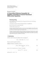
Figure 1: URA with N × P elements.
avoiding the estimation of a covariance matrix which leads
to enormous savings in the required real-time computations.
The performance of this algorithm is affected by the MC
effect, too [17] and must be compensated.
Unfortunately, the MC matrix tends to change with
timeduetoenvironmentalfactors,sofulleliminationof
its effect and prediction of its variability are impossible.
Therefore, calibration procedures based upon signal pro-
cessing algorithms are needed to estimate and compensate

for the effect of the MC. The most likely way is to
carry out some measurements for calibration. However, this
procedure has the drawbacks of being time-consuming and
very expensive [18]. Some other researches suggested self-
calibration adaptive algorithms for damping the MC effect
[19–21].
In this paper, a new adaptive algorithm was proposed for
the fast recovery of the signal with one snapshot of receiving
signals in the presence of mutual coupling, based on 2-
DD
3
LS algorithm for URA. Then, utilizing the 2-D D
3
LS
algorithm properties, a novel technique for the coupling
coefficients estimation, without using any auxiliary sensors
is presented.
This paper is organized as follows. Section 2,conven-
tional 2-D D
3
LS algorithm is reviewed. In Section 3,a
fast adaptive algorithm of direct data domain including
mutual coupling effect is presented. In Section 4,anew
technique is presented for compensation of the MC effect.
In Section 5, numerical simulations illustrate these proposed
techniques which can accurately recover the desired signal in
thepresenceofMC.
2. 2-D Direct Data Domain Algorithm
Consider a URA consisting of N × P equally spaced elements
with the spacing of d

x
in rows (in the x direction) and d
y
in
columns (in the y direction). The array receives a signal from
aknowndirection(θ
0
, ϕ
0
)andM interferers from unknown
directions (θ
m
, ϕ
m
), m = 1, 2, ,M as shown in Figure 1.
The output of the array voltage can be expressed as
x
= As + n,(1)
where x, A, s,andn denote the received signal vector,
steering matrix, signal plus jammers vector and additive
white Gaussian noise vector, respectively, defined as:
x
=
[
x
11
(
t
)
, x

12
(
t
)
, , x
1N
(
t
)
, x
21
(
t
)
, ,
x
2N
(
t
)
, , x
P1
(
t
)
, , x
PN
(
t
)]

T
,
s
=
[
s
(
t
)
, J
1
(
t
)
, J
2
(
t
)
, , J
M
(
t
)]
T
,
n
=
[
n

11
(
t
)
, n
12
(
t
)
, , n
1N
(
t
)
, n
21
(
t
)
, ,
n
2N
(
t
)
, , n
P1
(
t
)

, , n
PN
(
t
)]
T
,
A
=

a

θ
0
, ϕ
0

, a

θ
1
, ϕ
1

, , a

θ
M
, ϕ
M


,
(2)
where
a

θ
m
, ϕ
m

=
a
y

θ
m
, ϕ
m

⊗
a
x

θ
m
, ϕ
m

, m = 0, 1, 2, , M,

a
x

θ
m
, ϕ
m

=

1, β

θ
m
, ϕ
m

, , β
N−1

θ
m
, ϕ
m


T
,
a
y


θ
m
, ϕ
m

=

1, α

θ
m
, ϕ
m

, , α
P−1

θ
m
, ϕ
m


T
.
(3)
We de fine β(θ
m
, ϕ

m
) = exp( j2π(d
x
/λ)sinθ
m
cos ϕ
m
)and
α(θ
m
, ϕ
m
) = exp( j2π(d
y
/λ)sinθ
m
sin ϕ
m
) which represent
the phase progression of the signal between one element and
the next in the row and column, respectively. The a(θ
m
, ϕ
m
)is
mth signal’s direction manifold vector, superscript (
·)
T
is the
transpose operation and the symbol

⊗ denotes the Kronecker
tensor. Therefore, by suppression of time dependence in the
phasor notation, complex vector of phasor voltage is:
x
= s
0
a

θ
0
, ϕ
0

+
⎛
⎝
M

m=1
J
m
a

θ
m
, ϕ
m

⎞
⎠

+ n,(4)
where s
0
and J
m
are the complex amplitude of the desired
signal and mth interferers, respectively. Next, the first row
from each column is multiplied by β and subtracted from the
second row; then the result of each column is multiplied by α
and subtracted from the next column. This cancels out all the
signals and only noise and interferers are left. The first row of
the matrix in (5) is the constraint to the desired signal which
produces a gain factor of Q. For a conventional adaptive
array system, the K weights w
k
areusedandtherelationship
between K with P and N canbechosenasK
= K
1
· K
2
,
K
1
= (N +1)/2, K
2
= (P +1)/2[16]. Matrix equation can be
constructed as:
⎡
⎢

⎢
⎢
⎢
⎢
⎢
⎢
⎢
⎢
⎢
⎣
b
1
b
2
··· b
K
2
−1
b
K
2
D
1
D
2
··· D
(K
2
−1)
D

K
2
D
2
D
3
··· D
K
2
D
(K
2
+1)
.
.
.
D
(K
2
−1)
D
K
2
··· D
(P−2)
D
(P−1)
⎤
⎥
⎥

⎥
⎥
⎥
⎥
⎥
⎥
⎥
⎥
⎦
×
⎡
⎢
⎢
⎢
⎢
⎢
⎢
⎢
⎣
w
1
w
2
.
.
.
w
K
⎤
⎥

⎥
⎥
⎥
⎥
⎥
⎥
⎦
=
⎡
⎢
⎢
⎢
⎢
⎢
⎢
⎢
⎣
Q
0
.
.
.
0
⎤
⎥
⎥
⎥
⎥
⎥
⎥

⎥
⎦
,
(5)
where
b
1
=

1 β ··· β
K
1
−1

, b
i
= α
i−1
b
1
,(6)
EURASIP Journal on Wireless Communications and Networking 3
D
i
=
⎡
⎢
⎢
⎢
⎢

⎣

x
i1
− β
−1
x
i2

−
α
−1

x
(i+1)1
− β
−1
x
(i+1)2

···

x
iK
1
− β
−1
x
i(K
1

+1)

−
α
−1

x
(i+1)K
1
− β
−1
x
(i+1)(K
1
+1)

.
.
.
.
.
.

x
i(K
1
−1)
− β
−1
x

iK
1

−
α
−1

x
(i+1)(K
1
−1)
− β
−1
x
(i+1)K
1

···

x
i(N−1)
− β
−1
x
iN

−
α
−1


x
(i+1)(N−1)
− β
−1
x
(i+1)N

⎤
⎥
⎥
⎥
⎥
⎦
. (7)
For simplicity β(θ
0
, ϕ
0
) = β and α(θ
0
, ϕ
0
) = α.Becausethe
matrix in (5) is not square, the conjugate gradient method
(CGM) is used to solve the matrix equation and to obtain the
weighting solution. It has a good convergence characteristic
and converges to the minimum norm solution, even for the
singular problem [13]. Now, the amplitude of the recovered
signal is as [16]:
s

0
=
1
Q
K
1
K
2

i=1
w
i
x
i+[(i−1)/K
1
](K
1
−1)
,(8)
where w
= [w
1
, w
2
, , w
K
]
T
is the weights vector in the
absence of coupling and subscript, [

·], denotes rounding
down to the integer:
Q
=
K
1
K
2

i=1
α
[(i−1)/K
1
]
β
i−1−[(i−1)/K
1
]K
1
w
i
. (9)
3. 2-D Fast Sig nal Recovery Algorithm
in the Presence of Mutual Coupling
If one assumes that C denotes the mutual coupling matrix
(MCM) of the array, the output will be as:
x
= CAs + n,
(10)
x

= s
0
Ca

θ
0
, ϕ
0

+
⎛
⎝
M

m=1
J
m
Ca

θ
m
, ϕ
m

⎞
⎠
+ n. (11)
Svantesson [6] showed that the coupling between the
neighboring elements with the same interspace is almost the
same and the magnitude of the mutual coupling coefficient

between two far apart elements is so small that can be
approximated to zero. Thus, a banded symmetric Toeplitz
matrix can be used as a model for the mutual coupling of
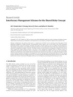
ULA and URA. In this paper, each sensor is assumed to be
affected by the coupling of the 8 sensors around it, which is
shown in Figure 2.
We d efin e M CM as [12]:
C
=
⎡
⎢
⎢
⎢
⎢
⎢
⎢
⎢
⎢
⎢
⎢
⎣
C
1
C
2
0 ··· 000
C
2
C
1

C
2
··· 000
.
.
.
.
.
.
.
.
.
.
.
.
000
··· C
2
C
1
C
2
000··· 0 C
2
C
1
⎤
⎥
⎥
⎥

⎥
⎥
⎥
⎥
⎥
⎥
⎥
⎦
PN×PN
, (12)
c
xy
c
y
c
xy
c
x
c
x
c
xy
c
y
c
xy
Figure 2: Map of mutual coupling.
where C
1
and C

2
are N×N submatrices of C and can be given
by
C
1
= To e p l i t z
([
1, c
x
,0, ,0
])
,
C
2
= To e p l i t z

c
y
, c
xy
,0, ,0

.
(13)
Then, the following equation is derived to recover the desired
signal in the presence of mutual coupling (Proof in the
appendix), notwithstanding to compute the inverse matrix of
MC. Hence, this equation could be reduced the computation
of the algorithm
s

0
=
1
Q
c
K
1
K
2

i=1
wc
i
· x
i+[(i−1)/K
1
](K
1
−1)
, (14)
where w
c
= [wc
1
, wc
2
, , wc
K
]
T

is the weights vector when
coupling is known and
Q
c
=

1+βc
x
+ αc
y
+ αβc
xy

K
1
K
2

i=1
α
[(i−1)/K
1
]
β
i−1−[(i−1)/K
1
]K
1
wc
i

+

c
x
+ αc
xy

(K
1
−1)K
2

i=1
α
[(i−1)/(K
1
−1)]
β
i−1−[(i−1)/(K
1
−1)](K
1
−1)
× wc
i+1+[(i−1)/(K
1
−1)]
4 EURASIP Journal on Wireless Communications and Networking
+


c
y
+ βc
xy

K
1
(K
2
−1)

i=1
α
[(i−1)/K
1
]
β
i−1−[(i−1)/K
1
]K
1
wc
i+K
1
+ c
xy
(K
1
−1)(K
2

−1)

i=1
α
[(i−1)/(K
1
−1)]
β
i−1−[(i−1)/(K
1
−1)](K
1
−1)
× wc
i+K
1
+1+[(i−1)/(K
1
−1)]
.
(15)
The conventional recovering of the signal is as the following:
s
0
=
1
Q

w
T


C
−1
x

K

, (16)
where [
·]
K
denotes, K rows from the vector. C
−1
is
computationally intensive and requires many calculations
in the real-time because evaluation of the inverse requires
an Θ([PN]
3
)process (here Θ(·) denotes “on the order of”).
Therefore, (14) can be replaced with (16)andthenumberof
processes would be an Θ(K
1
K
2
).
4. Mutual Coupling Compensation
In this section, a new method is presented to estimate the
coupling coefficients from the properties of the 2-D D
3
LS

algorithm. If the mutual coupling effect is ignored, the
term (x
ij
− β
−1
x
i(j+1)
) − α
−1
(x
(i+1) j
− β
−1
x
(i+1)( j+1)
), for i =
1, 2, ,P − 1and j = 1, 2, , N − 1willhavenosignal
components. However, in the presence of MC, for the edge
elements in the URA, the above term can be written as the
following:

x
11
− β
−1
x
12

−
α

−1

x
21
− β
−1
x
22

=
s
0
α
−1
β
−1
c
xy
+Interferers,

x
11
− β
−1
x
12

=−

β

−1
c
x
+ αβ
−1
c
xy

s
0
+Interferers,

x
11
− α
−1
x
21

=−

α
−1
c
y
+ α
−1
βc
xy


s
0
+Interferers,
(17)
As is seen in (17), when there are no interferers, the equations
can be solved. In this paper, it is assumed that d
x
= d
y
= d;
so c
x
= c
y
. The above equations can be solved in order
to estimate
c
x
, c
y
,andc
xy
. Once the system estimates the
coupling coefficient, it needs only one snapshot of the data in
order to obtain an acceptable solution. So, when the coupling
is unknown, first we can estimate mutual coupling from (17)
and then, the fast recovering of the signal is as the following:
s
0
=

1

Q
c
K
1
K
2

i=1
wc
i
· x
i+[(i−1)/K
1
](K
1
−1)
, (18)
where
s
0
is the estimation of s
0
and

Q
c
is Q
c

with replacement
of c
x
, c
y
, c
xy
with c
x
, c
y
, c
xy
.
5. Numerical Examples
In this section, the capability of MC compensation for
the proposed algorithm will be tested with two examples.
Table 1: Parameters for the desired signal and interferer.
Magnitude Phase θ
s
ϕ
s
Signal 1–10 V/m 0 75
◦
45
◦
Jammer1 1000 V/m 0 43
◦
−77
◦

10987654321
Intensities of the signal
1
2
3
4
5
6
7
8
9
10
Recovered of the signal
2D-D3LS without MC
2D-D3LS with MC
Figure 3: Recovered strength of the desired signal in the absence
and presence of mutual coupling.
Consider a URA with 7 × 7 elements in which the spacing
between each two elements in rows and columns is λ/2. The
array receives the desired signal with one jammer. The signal
to noise ratio is 20 dB and other parameters are listed in
Ta b l e 1.
The number of adaptive weights chosen for our simu-
lation will be 16 [16]. Jammer is 60 dB stronger than the
intensity of the desired signal. The magnitude of incident
signal varies from 1 V/m to 10 V/m; but jammer intensities
are constant as given in Ta b l e 1 . Figure 3 shows the accuracy
of the recovered signal in the presence of MC using new
formulation (18) with comparison to the ideal recovering.
Figure 4 shows the result of the recovered signal in the

presence of MC, using a new proposed algorithm with
comparison to the ideal recovering. The expected linear
relationship is clearly seen and the jammer has been nulled
and signal recovered correctly.
Later on, the performance of the proposed method is
illustrated by the various simulations. The amplitude of
the desired signal accuracy is measured by the root mean-
squared error (RMSE), and L
= 100 is the number of Monte
Carlo runs.
Figure 5 shows the RMSE of the estimated coupling
coefficients versus signal-to-noise ratio (SNR). Figure 6
shows the RMSE of the estimated amplitude of the desired
signal, versus SNR. For high SNR, error is very low and in
case there is no noise, new formulation is equal to the ideal.
EURASIP Journal on Wireless Communications and Networking 5
10987654321
Intensities of the signal
1
2
3
4
5
6
7
8
9
10
Recovered of the signal
Figure 4: Recovered strength of the desired signal with the

proposed algorithm in the presence of mutual coupling.
6. Conclusion
In this paper, the problems of 2-D D
3
LS algorithms were
studied for recovering of the signal in the presence of mutual
coupling and driving a new formulation to recover the signal
in the presence of MC. Without using the moment of method
and impedance matrix calculation, coupling coefficients
can be automatically estimated and without computing the
inverse matrix, the desired signal can be recovered. Because
we did not use the inverse MC matrix, the amount of
computation would be reduced. Moreover, simulation results
were confirmed when SNR was high and the RMSE of the
method was very close to the ideal D
3
LS in the absence of
MC.
Appendix
In this appendix, (8)and(14) are proved. Consider a URA
consisting of 5
× 5 elements. The array receives one signal (s)
from a known direction (θ
0
, ϕ
0
) and one interferer ( j)(this
proof can be extended similarly). From (1), let the received
signal at the array in the presence of mutual coupling for each
element be

x
np
= s
np
+ j
np
,for

n = 1, ,5, p = 1, ,5

,(A.1)
where s
np
, j
np
are the received signal and jammer at the npth
element, expressed as
s
11
= s = g
s
e
jwt
, s
n(p+1)
= βs
np
, s
(n+1)p
= αs

np
.
(A.2)
40353025201510
S/N (dB)
0
5
10
15
20
25
30
RMSE (%) of coupling coefficient
c
x
, c
y
c
xy
Figure 5: RMSE of the coupling coefficients versus the SNR.
40353025201510
S/N (dB)
0
2
4
6
8
10
12
14

16
18
20
RMSE (%) of amplitude of recovered signal
Ideal D3LS
Proposed algorithm
Figure 6: RMSE of the recovered amplitude versus the SNR.
By taking mutual coupling into account, from (11)foreach
column
first column:
s
11
=

1+βc
x
+ αc
y
+ αβc
xy

s,
s
12
= βs
11
+

c
x

+ αc
xy

s,
s
1p
= βs
1(p−1)
,forp = 3, 4, 5,
2nd column:
s
21
= αs
11
+

c
y
+ βc
xy

s,
6 EURASIP Journal on Wireless Communications and Networking
s
22
= βs
21
+

c

xy
+ αc
x
+ α
2
c
xy

s,
s
2p
= βs
2(p−1)
,forp = 3, 4,5,
3rd column:
s
31
= αs
21
,
s
32
= βs
31
+ α

c
xy
+ αc
x

+ α
2
c
xy

s,
s
3p
= βs
3(p−1)
,forp = 3, 4,5,
4th column:
s
41
= αs
31
,
s
42
= βs
41
+ α
2

c
xy
+ αc
x
+ α
2

c
xy

s,
s
4p
= βs
4(p−1)
,forp = 3, 4,5.
(A.3)
(a) Absence of the Mutual Coupling. If the one row from each
column is multiplied by β and subtracted from the next row
and then the result of each column is multiplied by α and
subtracted from the next column, in the absence of mutual
coupling, this will cancel out all the signals and only noise
and interferer will be left

x
np
− β
−1
x
n(p+1)

−
α
−1

x
(n+1)p

− β
−1
x
(n+1)(p+1)

,
for n
= 1, 2, ,4, p = 1, 2, ,4.
(A.4)
The weight vectors should be in a way that produces zero
output; therefore, a reduced rank matrix is formed in which
the weighted sum of all its elements would be zero. In order
to make the matrix not singular, the additional equation
is introduced through the constraint that the same weights
when operating on the signal produced a gain factor Q,
which is the first equation. Therefore, (5)willbe
⎡
⎢
⎢
⎢
⎣
b
1
b
2
b
3
D
1
D

2
D
3
D
2
D
3
D
4
⎤
⎥
⎥
⎥
⎦
×
⎡
⎢
⎢
⎢
⎢
⎢
⎢
⎢
⎣
w
1
w
2
.
.

.
w
9
⎤
⎥
⎥
⎥
⎥
⎥
⎥
⎥
⎦
=
⎡
⎢
⎢
⎢
⎢
⎢
⎢
⎢
⎣
Q
0
.
.
.
0
⎤
⎥

⎥
⎥
⎥
⎥
⎥
⎥
⎦
,(A.5)
⎡
⎢
⎢
⎢
⎢
⎢
⎢
⎢
⎢
⎢
⎢
⎢
⎢
⎣
1 ··· β
2

x
11
− β
−1
x

12

−
α
−1

x
21
− β
−1
x
22

···

x
13
− β
−1
x
14

−
α
−1

x
23
− β
−1

x
24


x
12
− β
−1
x
13

−
α
−1

x
22
− β
−1
x
23

···

x
14
− β
−1
x
15


−
α
−1

x
24
− β
−1
x
25


x
21
− β
−1
x
22

−
α
−1

x
31
− β
−1
x
32


···

x
23
− β
−1
x
24

−
α
−1

x
33
− β
−1
x
34


x
22
− β
−1
x
23

−

α
−1

x
32
− β
−1
x
33

···

x
24
− β
−1
x
25

−
α
−1

x
34
− β
−1
x
35


α ··· αβ
2

x
21
− β
−1
x
22

−
α
−1

x
31
− β
−1
x
32

···

x
23
− β
−1
x
24


−
α
−1

x
33
− β
−1
x
34


x
22
− β
−1
x
23

−
α
−1

x
32
− β
−1
x
33


···

x
24
− β
−1
x
25

−
α
−1

x
34
− β
−1
x
35


x
31
− β
−1
x
32

−
α

−1

x
41
− β
−1
x
42

···

x
33
− β
−1
x
34

−
α
−1

x
43
− β
−1
x
44



x
32
− β
−1
x
33

−
α
−1

x
42
− β
−1
x
43

···

x
34
− β
−1
x
35

−
α
−1


x
44
− β
−1
x
45

α
2
··· α
2
β
2

x
31
− β
−1
x
32

−
α
−1

x
41
− β
−1

x
42

···

x
33
− β
−1
x
34

−
α
−1

x
43
− β
−1
x
44


x
32
− β
−1
x
33


−
α
−1

x
42
− β
−1
x
43

···

x
34
− β
−1
x
35

−
α
−1

x
44
− β
−1
x

45


x
41
− β
−1
x
42

−
α
−1

x
51
− β
−1
x
52

···

x
43
− β
−1
x
44


−
α
−1

x
53
− β
−1
x
54


x
42
− β
−1
x
43

−
α
−1

x
52
− β
−1
x
53


···

x
44
− β
−1
x
45

−
α
−1

x
54
− β
−1
x
55

⎤
⎥
⎥
⎥
⎥
⎥
⎥
⎥
⎥
⎥

⎦
×
⎡
⎢
⎢
⎢
⎢
⎢
⎢
⎢
⎢
⎣
w
1
w
2
.
.
.
w
9
⎤
⎥
⎥
⎥
⎥
⎥
⎥
⎥
⎥

⎦
=
⎡
⎢
⎢
⎢
⎢
⎢
⎢
⎢
⎢
⎣
Q
0
.
.
.
0
⎤
⎥
⎥
⎥
⎥
⎥
⎥
⎥
⎥
⎦
.
(A.6)

EURASIP Journal on Wireless Communications and Networking 7
Then, performing the matrix multiplication in (A.6)forthe
first row of the matrix will give
w
1
+ βw
2
+ β
2
w
3
+ αw
4
+ αβw
5
+ αβ
2
w
6
+ α
2
w
7
+ α
2
βw
8
+ α
2
β

2
w
9
= Q.
(A.7)
With performing the matrix multiplication in (A.6)forthe
second row of the matrix the following is obtained:

x
11
− β
−1
x
12

−
α
−1

x
21
− β
−1
x
22

w
1
+


x
12
− β
−1
x
13

−
α
−1

x
22
− β
−1
x
23

w
2
+

x
13
− β
−1
x
14

−

α
−1

x
23
− β
−1
x
24

w
3
+

x
21
− β
−1
x
22

−
α
−1

x
31
− β
−1
x

32

w
4
+

x
22
− β
−1
x
23

−
α
−1

x
32
− β
−1
x
33

w
5
+

x
23

− β
−1
x
24

−
α
−1

x
33
− β
−1
x
34

w
6
+

x
31
− β
−1
x
32

−
α
−1


x
41
− β
−1
x
42

w
7
+

x
32
− β
−1
x
33

−
α
−1

x
42
− β
−1
x
43


w
8
+

x
33
− β
−1
x
34

−
α
−1

x
43
− β
−1
x
44

w
9
= 0.
(A.8)
So

j
11

w
1
+ j
12
w
2
+ j
13
w
3
+ j
21
w
4
+ j
22
w
5
+j
23
w
6
+ j
31
w
7
+ j
32
w
8

+ j
33
w
9

−
β
−1

j
12
w
1
+ j
13
w
2
+ j
14
w
3
+ j
22
w
4
+ j
23
w
5
+j

24
w
6
+ j
32
w
7
+ j
33
w
8
+ j
34
w
9

−
α
−1

j
21
w
1
+ j
22
w
2
+ j
23

w
3
+ j
31
w
4
+ j
32
w
5
+j
33
w
6
+ j
41
w
7
+ j
42
w
8
+ j
43
w
9

+ α
−1
β

−1

j
22
w
1
+ j
23
w
2
+ j
24
w
3
+ j
32
w
4
+ j
33
w
5
+j
34
w
6
+ j
42
w
7

+ j
43
w
8
+ j
44
w
9

=
0.
(A.9)
Az α
−1
/
= 0, β
−1
/
= 0, and w
i
/
= 0, (A.9)willbetrueforallw
if and only if each summation in the parenthesis is equal to
zero. Therefore, the first summation will be used
j
11
w
1
+ j
12

w
2
+ j
13
w
3
+ j
21
w
4
+ j
22
w
5
+ j
23
w
6
+ j
31
w
7
+ j
32
w
8
+ j
33
w
9

= 0.
(A.10)
Similarly, the same can be done for the third row of the
matrix (A.5), and so forth. In the absence of mutual coupling
(c
x
= c
y
= c
xy
= 0). From (A.3)and(A.10)
(
x
11
− s
11
)
· w
1
+

x
12
− βs
11

·
w
2
+


x
13
− β
2
s
11

·
w
3
+
(
x
21
− αs
11
)
· w
4
+

x
22
− αβs
11

·
w
5

+

x
23
− αβ
2
s
11

·
w
6
+

x
31
− α
2
s
11

·
w
7
+

x
32
− α
2

βs
11

·
w
8
+

x
33
− α
2
β
2
s
11

·
w
9
= 0.
(A.11)
Then, (A.11) will be as simple as
(
x
11
w
1
+ x
12

w
2
+ x
13
w
3
)
+
(
x
21
w
4
+ x
22
w
5
+ x
23
w
6
)
+
(
x
31
w
7
+ x
32

w
8
+ x
33
w
9
)
= s

w
1
+ βw
2
+ β
2
w
3

+

αw
4
+ αβw
5
+ αβ
2
w
6

+


α
2
w
7
+ α
2
βw
8
+ α
2
β
2
w
9

=⇒
9

i=1
w
i
x
i+2[(i−1)/3]
= sQ
.
(A.12)
Therefore, the desired signal can be recovered by
s
=

1
Q
K
2
K
1

i=1
w
i
x
i+[(i−1)/K
1
](K
1
−1)
. (A.13)
(b) Presence of the Mutual Coupling. When there is mutual
coupling, the matrix (A.5) can be formed and the (A.3)and
(A.10)canbewritteninasimilarway
(
x
11
− s
11
)
· w
1
+


x
12
− βs
11
−

c
x
+ αc
xy

s

·
w
2
+

x
13
− β
2
s
11
− β

c
x
+ αc
xy


s

·
w
3
+

x
21
− αs
11
−

c
y
+ βc
xy

s

·
w
4
+

x
22
− αβs
11

− β

c
y
+ βc
xy

s
−

c
xy
+ αc
x
+ α
2
c
xy

s

·
w
5
+

x
23
− αβ
2

s
11
− β
2

c
y
+ βc
xy

s
−β

c
xy
+ αc
x
+ α
2
c
xy

s

·
w
6
+

x

21
− α
2
s
11
− α

c
y
+ βc
xy

s

·
w
7
+

x
22
− α
2
βs
11
− αβ

c
y
+ βc

xy

s
−α

c
xy
+ αc
x
+ α
2
c
xy

s

·
w
8
+

x
23
− α
2
β
2
s
11
− αβ

2

c
y
+ βc
xy

s
−αβ

c
xy
+ αc
x
+ α
2
c
xy

s

·
w
9
= 0.
(A.14)
8 EURASIP Journal on Wireless Communications and Networking
Similar to (A.11), the following can be presented
(
x

11
w
1
+ x
12
w
2
+ x
13
w
3
)
+
(
x
21
w
4
+ x
22
w
5
+ x
23
w
6
)
+
(
x

31
w
7
+ x
32
w
8
+ x
33
w
9
)
=

1+βc
x
+ αc
y
+ αβc
xy

×
s

w
1
+ βw
2
+ β
2

w
3

+

αw
4
+ αβw
5
+ αβ
2
w
6

+

α
2
w
7
+ α
2
βw
8
+ α
2
β
2
w
9


+

c
x
+ αc
xy

×
s

w
2
+ βw
3
+ αw
5
+ αβw
6
+ α
2
w
8
+ α
2
βw
9

+


c
y
+ βc
xy

s

w
4
+ βw
5
+ β
2
w
6
+ αw
7
+ αβw
8
+ αβ
2
w
9

+

c
xy

s


w
5
+ βw
6
+ αw
8
+ αβw
9

.
(A.15)
The recovered signal will be as follows:
=⇒
9

i=1
w
i
x
i+2[(i−1)/3]
= s
⎡
⎣

1+βc
x
+ αc
y
+ αβc

xy

9

i=1
α
[(i−1)/3]
β
i−1−3[(i−1)/3]
wc
i
+

c
x
+ αc
xy

6

i=1
α
[(i−1)/2]
β
i−1−2[(i−1)/2]
wc
i+1+[(i−1)/2]
+

c

y
+ βc
xy

6

i=1
α
[(i−1)/3]
β
i−1−[(i−1)/3]K
1
wc
i+3
+c
xy
4

i=1
α
[(i−1)/2]
β
i−1−2[(i−1)/2]
wc
i+4+[(i−1)/2]
⎤
⎦
.
(A.16)
Acknowledgment

The authors want to acknowledge the Iran Telecommunica-
tion Research Centre (ITRC) for their kindly supports.
References
[1]T.Nishimura,H.P.Bui,H.Nishimoto,Y.Ogawa,and
T. Ohgane, “Channel characteristics and performance of
MIMO E-SDM systems in an indoor time-varying fading
environment,” Eurasip Journal on Wireless Communications
and Networking, vol. 2010, Article ID 736962, 14 pages,
2010.
[2]I.J.GuptaandA.A.Ksienski,“Effect of mutual coupling
on the performance of adaptive array,” IEEE Transactions
on Ante nnas and Propagation, vol. 31, no. 5, pp. 785–791,
1983.
[3] B. Friedlander and A. J. Weiss, “Direction finding in the
presence of mutual coupling,” IEEE Transactions on Antennas
and Propagation, vol. 39, pp. 273–284, 1991.
[4] E. M. Friel and K. M. Pasala, “Effects of mutual coupling on
the performance of STAP antenna arrays,” IEEE Transactions
on Aerospace and Electronic Systems, vol. 36, no. 2, pp. 518–
527, 2000.
[5] H.S.LuiandH.T.Hui,“Mutualcouplingcompensationfor
direction-of-arrival estimations using the receiving-mutual-
impedance method,” International Journal of Antennas and
Propagation, vol. 2010, Article ID 373061, 7 pages, 2010.
[6] T. Svantesson, “Modeling and estimation of mutual coupling
in a uniform linear array of dipoles,” Tech. Rep. S-412 96,
Dept. Signals and Systems, Chalmers Univ. of Tech., Sweden,
1999.
[7]C.K.E.Lau,R.S.Adve,andT.K.Sarkar,“Minimumnorm
mutual coupling compensation with applications in direction

of arrival estimation,” IEEE Transact ions on Antennas and
Propagation, vol. 52, no. 8, pp. 2034–2041, 2004.
[8] Z.Huang,C.A.Balanis,andC.R.Britcher,“Mutualcoupling
compensation in UCAs: simulations and experiment,” IEEE
Transactions on Antennas and Propagation, vol. 54, no. 11,
pp. 3082–3086, 2006.
[9]T.T.Zhang,Y.L.Lu,andH.T.Hui,“Compensationforthe
mutual coupling effect in uniform circular arrays for 2D DOA
estimations employing the maximum likelihood technique,”
IEEE Transact ions on Aerospace and Electronic Systems,vol.44,
no. 3, pp. 1215–1221, 2008.
[10] M. D. Zoltowski, M. Haardt, and C. P. Mathews, “Closed-form
2-D angle estimation with rectangular arrays in element space
or beamspace via unitary ESPRIT,” IEEE Tr ansactions on Signal
Processing, vol. 44, no. 2, pp. 316–328, 1996.
[11] J. Liu and X. Liu, “Joint 2-D DOA tracking for multiple
moving targets using adaptive frequency estimation,” in
Proceedings of IEEE International Conference on Acoustics,
Speech and Signal Processing (ICASSP ’07), vol. 2, pp. 1113–
1116, 2007.
[12] Z. Ye and C. Liu, “2-D DOA estimation in the presence
of mutual coupling,” IEEE Transactions on Antennas and
Propagation, vol. 56, no. 10, pp. 3150–3158, 2008.
[13] T. K. Sarkar and N. Sangruji, “Adaptive nulling system
for a narrow-band signal with a look-direction constraint
utilizing the conjugate gradient method,” IEEE Transactions
on Antennas and Propagation, vol. 37, no. 7, pp. 940–944,
1989.
[14] T. K. Sarkar, H. Wang, S. Park et al., “A deterministic least-
squares approach to space-time adaptive processing (STAP),”

IEEE Transactions on Antennas and Propagation, vol. 49, no. 1,
pp. 91–103, 2001.
[15]T.Sarkar,M.Wicks,M.Palma,andR.Bonneau,Smart
Antennas, Wiley, New York, NY, USA, 2003.
[16] L. L. Wang and DA. G. Fang, “Modified 2-D direct data
domain algorithm in adaptive antenna arrays,” in Proceedings
of Asia-Pacific Microwave Conference (APMC ’05), December
2005.
[17] R. S. Adve and T. K. Sarkar, “Compensation for the effects of
mutual coupling on direct data domain adaptive algorithms,”
IEEE Transactions on Antennas and Propagation, vol. 48, no. 1,
pp. 86–94, 2000.
[18] B. Wang, Y. Wang, and Y. Guo, “Mutual coupling calibration
with instrumental sensors,”
Electronics Letters, vol. 40, no. 7,
pp. 406–408, 2004.
[19] Y. Horiki and E. H. Newman, “A self-calibration technique
for a DOA array with near-zone scatterers,” IEEE Transactions
on Antennas and Propagation, vol. 54, no. 4, pp. 1162–1166,
2006.
EURASIP Journal on Wireless Communications and Networking 9
[20] F. Sellone and A. Serra, “A novel online mutual coupling
compensation algorithm for uniform and linear arrays,” IEEE
Transactions on Signal Processing, vol. 55, no. 2, pp. 560–573,
2007.
[21] Z. Ye and C. Liu, “On the resiliency of MUSIC direction
finding against antenna sensor coupling,” IEEE Tr ansactions
on Ante nnas and Propagation, vol. 56, no. 2, pp. 371–380,
2008.