Báo cáo hóa học: " Research Article Computationally Efficient DOA and Polarization Estimation of Coherent Sources with Linear Electromagnetic Vector-Sensor Array" ppt
Bạn đang xem bản rút gọn của tài liệu. Xem và tải ngay bản đầy đủ của tài liệu tại đây (1.14 MB, 10 trang )
Hindawi Publishing Corporation
EURASIP Journal on Advances in Signal Pr ocessing
Volume 2011, Article ID 490289, 10 pages
doi:10.1155/2011/490289
Research Ar ticle
Computationally Efficient DOA and Polarization
Estimation of Coherent Sources with
Linear Elect romagnetic Vector-Sensor Array
Zhaoting Liu,
1
Jing He,
2
and Zhong Liu
1
1
Department of Electronic Engineering, Nanjing University of Science and Technology, Nanjing, Jiangsu 210094, China
2
Department of Electr ical and Computer Engineering, Concordia University, Montreal, QC, Canada H3G 2W1
Correspondence should be addressed to Zhaoting Liu,
Received 3 September 2010; Revised 10 December 2010; Accepted 16 January 2011
Academic Editor: Ana P
´
erez-Neira
Copyright © 2011 Zhaoting Liu et al. This is an open access article distributed under the Creative Commons Attribution License,
which permits unrestricted use, distribution, and r eproduction in any medium, provided the original work is properly
cited.
This paper studies the problem of direction finding and polarization estimation of coherent sources using a uniform
linear electromagnetic vector-sensor (EmVS) array. A novel preproc essing algorithm based on Em VS subarray averaging
(EVSA) is firstly proposed to decorrelate s ources’ coherency. Then, the proposed EVSA algorithm is combined with the
propagator method (PM) to estimate the EmVS steering vector, and thus estimate the direction-of-arrival (DOA) and the
polarization parameters by a vector cross-product operation. Compared with the existing estimate methods, the proposed
EVSA-PM enables decorrelation of m ore coherent signals, joint estimation of the DOA and polarization of coherent
sources with a lower computational complexity, and requires no limitation of the intervector sensor spacing within a
half-wavelength to guarantee unique and unambiguous angle estimates. Also, the EVSA-PM can estimate these parameters
by parameter-space searching techniques. Monte-Carlo simulations are presented to verify the efficacy of the proposed
algorithm.
1. Introduction
A ty pical electromagnetic vector-sensor (EmVS) consists
of six component sensors configured by two orthogonal
triads of dipole and loop antennas with the same phase
center. Therefore, an EmVS can simultaneously measure
the three components of the electric field and the three
components of the magnetic field. Since its introduction into
signal processing community [1, 2], a significant number
of research has been done on EmVS array processing
[3–19]. For application considerations, different types of
EmVS containing part of the six sensors are devised and
manufactured [3, 20, 21].
In the study of direction finding applications, conven-
tional eigenstructure-based source localization techniques
have been extended to the case of the EmVS array. ESPRIT/
MUSIC algorithms using EmVS arrays obtain thorough
in vestigations [10–12, 16–19]. The signal subspace and
noise subspace are usually constructed by decomposing
the column space of the data correlation matrix with
the eigen-decomposition (or singular value decomposition)
techniques [22, 23]. Because the decomposing p rocess is
computationally intensive and t ime consuming, t he eigen-
structure-based techniques may be unsuitable for many
practical situations, especially when the number of vector
sensors is large and/or the directions of impinging sources
should be tracked in an o nline manner.
Furthermore, the eigenstructure-based direction finding
techniques using the EmVS arrays usually assume incoherent
signals, that is, that the signal covariance matrix has full rank.
This assumption is often violated in scenarios where multi-
path exists. Coherent signals could reduce the rank of signal
covariance matrix below the number of incident signals,
and hence, degrade critically the algorithmic performance.
2 EURASIP Journal on Advances in Signal Pr ocessing
To deal with the coherent signals using the EmVS array, a
polarization smoothing algorithm (PSA) has been proposed
to restore the rank of signal subspace [19]. The PSA does not
reduce the effective array aperture length and has no limit to
array geometries. However, the PSA-based method has non-
negligible drawbacks. (1) It assumes the intervector sensor
spacing within a half-wavelength to guarantee unique and
unambiguous angle estimates; (2) it is not able to estimate
the polarization of impinging electromagnetic waves; (3)
the EmVS type limits the maximum number of resolvable
coherent signals.
In this paper, we employ a uniform linear EmVS
array to perform parameter estimation of coherent sources.
Firstly, to decorrelate the co her ent sources, an EmVS sub-
array averaging-based pre-processing (EVSA) algorithm is
developed. Then the EVSA algorithm is coupled with the
propagator method (PM) [24, 25] to estimate parameters
of the coherent sources without eigen-decomposition or
singular value decomposition unlike the ESPRIT/MUSIC-
based methods. By using the vector cross-product o f the
electric field vector estimate and the magnetic field vector
estimate, the proposed EVSA-PM can estimate both the
DOA and polarization parameters, hence, can overcome the
drawbacks of the PSA-based algorithms to some extent. The
vector cross-product estimator is valid to a six-component
EmVS array. For the array comprising any t ypes of EmVSs,
the EVSA-PM with parameter-space searching techniques
is developed to estimate the parameters. The EVSA-PM
can be regarded as an extension of the subspace-based
method without eigendecomposition (SUMWE) [26]tothe
case of the EmVS arrays. The SUMWE is also a PM-based
method, which estimates the DOA of coherent sources using
unpolarized scalar sensors by an iterative angle searching.
However, the proposed methods make use of more available
electromagnetic information, and hence, should outperform
the SUMWE algorithm in accuracy and resolution of DOA
estimation.
The rest of this paper is organized as follows. Section 2
formulates the mathematical data model of EmVS array.
Section 3 develops the proposed EmVS-PM. Section 4
presents the simulation results to verify the efficacy of the
EmVS-PM. Section 5 concludes the paper.
2. Mathematical Data Model
Assume that K narrowband completely polarized coherent
signals impinge upon a uniform linear EmVS array with M
vector sensors (M>2K), and the array is neither mutual
coupling nor cross-polarization effects. The K is known
in advance and the kth incident source is parameterized
{θ
k
, ϕ
k
, γ
k
, η
k
},where0≤ θ
k
≤ π/2 denotes the kth source’s
elevation angle measured from the vertical z-axis, 0
≤ ϕ
k
≤
2π represents the kth source’s azimuth angle, 0 ≤ γ
k
≤ π/2
refers to the kth source’s auxiliary polarization angle, and
−π ≤ η
k
≤ π symbolizes the kth source’s polarization phase
difference. For a six-component EmVS, the steering vector of
the kth unit-power electromagnetic source signal produces
the following 6
× 1vector:
c
θ
k
, ϕ
k
, γ
k
, η
k
def
=
⎡
⎢
⎢
⎢
⎢
⎢
⎢
⎢
⎢
⎢
⎢
⎢
⎢
⎣
c
1,k
c
2,k
c
3,k
c
4,k
c
5,k
c
6,k
⎤
⎥
⎥
⎥
⎥
⎥
⎥
⎥
⎥
⎥
⎥
⎥
⎥
⎦
def
=
⎡
⎢
⎢
⎢
⎢
⎢
⎢
⎢
⎢
⎢
⎢
⎢
⎢
⎣
e
x,k
e
y,k
e
z,k
h
x,k
h
y,k
h
z,k
⎤
⎥
⎥
⎥
⎥
⎥
⎥
⎥
⎥
⎥
⎥
⎥
⎥
⎦
=
⎡
⎢
⎢
⎢
⎢
⎢
⎢
⎢
⎢
⎢
⎢
⎢
⎢
⎣
cos ϕ
k
cos θ
k
− sin ϕ
k
sin ϕ
k
cos θ
k
cos ϕ
k
− sin θ
k
0
− sin ϕ
k
− cos ϕ
k
cos θ
k
cos ϕ
k
− sin ϕ
k
cos θ
k
0sinθ
k
⎤
⎥
⎥
⎥
⎥
⎥
⎥
⎥
⎥
⎥
⎥
⎥
⎥
⎦
def
= Θ
(
θ
k
,φ
k
)
⎡
⎣
sin γ
k
e
jη
k
cos γ
k
⎤
⎦
def
= g
(
γ
k
,η
k
)
,
(1)
where e
k
def
= [e
x,k
, e
y,k
, e
z,k
]
T
and h
k
def
= [h
x,k
, h
y,k
, h
z,k
]
T
denote the electric field vector and the magnetic field vector,
respectively .
The intersensor spatial phase factor for the kth inci-
dent signal and the mth vector sensor is q
m
(θ
k
, ϕ
k
)
def
=
e
j2π(x
m
u
k
+y
m
v
k
)/λ
,whereu
k
def
= sin θ
k
cos ϕ
k
and v
k
def
=
sin θ
k
sin ϕ
k
signify the direction cosines along the x-axis
and y-axis, respectively. (x
m
, y
m
) is the location of the mth
vector sensor, λ equals the signals’ wavelength. Denoting the
spacing between adjacent vector sensors as (Δ
x
, Δ
y
), we have
x
m
= x
1
+(m − 1)Δ
x
, y
m
= y
1
+(m − 1)Δ
y
.The6× 1
measurement vector corresponding to the mth vector sensor
can be expressed as
x
m
(
t
)
def
=
x
m,1
(
t
)
, , x
m,6
(
t
)
T
=
K
k=1
q
m
θ
k
, ϕ
k
c
θ
k
, ϕ
k
, γ
k
, η
k
s
k
(
t
)
+ w
m
(
t
)
,
(2)
where w
m
(t) = [w
m,1
(t), , w
m,6
(t)]
T
is the additive zero-
mean complex noise and independent to all signals. x
m,n
(t)
and w
m,n
(t) refer to the measurement and the noise corre-
sponding to the mth vector sensor’s nth component, respec-
tively; s
k
(t)representsthekth source’s complex envelope.
Without loss of generality, we consider the signals
{s
k
(t)} are
all coherent so that they are all some complex multiples of a
common signal s
1
(t). Then, under the flat-fading multipath
propagation, they can be expressed as s
k
(t) = β
k
s
1
(t)[26, 27],
where β
k
is the multipath coefficientthatrepresentsthe
complex attenuation of the kth signal with respect to the first
one (β
1
= 1andβ
k
/
= 0).
EURASIP Journal on Advances in Sig nal Processing 3
For the entire vector-sensor array, the array manifold,
a(θ
k
, ϕ
k
, γ
k
, η
k
) ∈ C
6M×1
,isgivenby
a
θ
k
, ϕ
k
, γ
k
, η
k
def
= q
θ
k
, ϕ
k
⊗
c
θ
k
, ϕ
k
, γ
k
, η
k
,(3)
where
⊗ symbolizes the Kronecker product operator,
q(θ
k
, ϕ
k
)
def
= [q
1
(θ
k
, ϕ
k
), , q
M
(θ
k
, ϕ
k
)]
T
.WithatotalofK
signals, the entire 6M
× 1 output vector measured by the
EmVS array at time t has the complex envelope represented
as
z
(
t
)
=
x
T
1
(
t
)
, , x
T
M
(
t
)
T
=
K
k=1
a
θ
k
, ϕ
k
, γ
k
, η
k
s
k
(
t
)
+ n
(
t
)
= As
(
t
)
+ n
(
t
)
,
(4)
where A
∈ C
6M×K
, s(t) ∈ C
K×1
, n(t) ∈ C
6M×1
,andA =
[a(θ
1
, ϕ
1
, γ
1
, η
1
), , a(θ
K
, ϕ
K
, γ
K
, η
K
)]; s(t) = [s
1
(t), ,
s
K
(t)]
T
, n(t) = [w
T
1
(t), , w
T
M
(t)]
T
.
3. Algorithm Development
This section is devoted to the algorithm de velopment.
Section 3.1 develops the EVSA algorithm, Section 3.2
describes EVSA-PM algorithm for estimating both DOA and
polarization parameters from the available EmVS steering
vector estimates and Section 3.3 is for parameters estimation
by parameter-space searc hing techniques.
3.1. EVSA Algorithm. Let us consider the subarray averaging
scheme with a linear EmVS array, which is divided into
L overlapping subarrays with K vector sensors and the lth
subarray comprises the lth to (l + K
− 1)th vector sensor,
where L
= M − K + 1. We use the first vector sensor as
a reference ( x
1
= 0, y
1
= 0), and then the corresponding
6K
× 1 signal vector is given as
z
l
(
t
)
def
=
x
T
l
(
t
)
, , x
T
l+K
−1
(
t
)
T
= A
0
D
l−1
s
(
t
)
+ n
l
(
t
)
,(5)
where D
∈ C
K×K
,andD
def
= diag(e
j2π(Δ
x
u
1
+Δ
y
v
1
)/λ
, ,
e
j2π(Δ
x
u
K
+Δ
y
v
K
)/λ
); A
0
∈ C
6K×K
contains the first 6K rows of A;
n
l
(t)
def
= [w
T
l
(t), , w
T
l+K
−1
(t)]
T
. We can calculate the cross-
correlation vector ϕ
l,n
∈ C
6K×1
between z
l
(t)andx
M,n
(t)
ϕ
l,n
def
= E
z
l
(
t
)
x
∗
M,n
(
t
)
=
A
0
D
l−1
E
s
(
t
)
s
H
(
t
)
a
∗
M,n
+ E
n
l
(
t
)
w
∗
M,n
=
ρ
M,n
r
s
A
0
D
l−1
β, l = 1, , L − 1; n = 1, ,6,
(6)
where E
{·} denotes the expectation, r
s
def
= E{s
1
(t)s
∗
1
(t)},
ρ
l,n
def
= β
H
a
∗
l,n
, a
l,n
def
= [q
l
(θ
1
, ϕ
1
)c
n,1
, ,q
l
(θ
K
, ϕ
K
)c
n,K
]
T
,
β
def
=
[β
1
, , β
K
]
T
. Similarly, the cross-correlation vector
ϕ
l,n
∈ C
6K×1
between z
l
(t)andx
1,n
(t) is as follows
ϕ
l,n
def
= E
z
l
(
t
)
x
∗
1,n
(
t
)
=
ρ
1,n
r
s
A
0
D
l−1
β, l = 2, , L; n = 1, ,6.
(7)
Let us rewrite the vector ϕ
l,n
as a 6 × K matrix
Φ
l,n
def
=
J
1
ϕ
l,n
, , J
K
ϕ
l,n
=
ρ
M,n
r
s
A
1
D
l−1
β, ,
A
K
D
l−1
β
=
ρ
M,n
r
s
A
l
β, , D
K−1
β
=
ρ
M,n
r
s
A
l
BQ
T
,
(8)
where J
k
def
= [0
6,6(k−1)
, I
6
, 0
6,6(K−k)
]; B
def
= diag(β
1
, , β
K
);
A
l
is the 6 × K matrix with the column c
k
q
l
(θ
k
, ϕ
k
),
k
= 1, ,6; Q is the K × K matrix with the column
[q
1
(θ
k
, ϕ
k
), , q
K
(θ
k
, ϕ
k
)]
T
. Similarly, the vector ϕ
l,n
can be
rewritten as
Φ
l,n
def
=
J
1
ϕ
l,n
, , J
K
ϕ
l,n
=
ρ
1,n
r
s
A
l
BQ
T
. (9)
Therefore, concatenating Φ
l,n
for l = 1, , L − 1and
Φ
l,n
for
l
= 2, , L, respectively, we can get two correlation matrices
R
n
def
=
Φ
T
1,n
, Φ
T
2,n
, , Φ
T
(
L
−1
)
,n
T
= ρ
M,n
r
s
ABQ
T
,
R
n
def
=
Φ
T
2,n
,
Φ
T
3,n
, ,
Φ
T
L,n
T
= ρ
1,n
r
s
ABDQ
T
,
(10)
where R
n
∈ C
6(L−1)×K
,
R
n
∈ C
6(L−1)×K
,and
A
def
= [
A
T
1
, ,
A
T
L
−1
]
T
includes the first 6(L − 1) rows of A.With(10), the
EmVS subarray averaging (EVSA) matrix can be formulated
as
R
def
=
R
1
, , R
6
,
R
1
, ,
R
6
=
AΩ, (11)
where Ω
def
= r
s
B[ρ
M,1
Q
T
, , ρ
M,6
Q
T
, ρ
1,1
DQ
T
, , ρ
1,6
DQ
T
].
Note that B and D are diagonal matrices with nonzero
diagonal elements, and Q is full rank when all sources
impinge with the distinct incident directions. Then the R
n
and
R
n
are of rank K, and hence, R is of rank K and can be
used to estimate the DOA and the polarization parameters of
the coherent sources.
In realistic cases where only a finite number of snapshots
are available, the cross-correlation vector ϕ
l,n
and ϕ
l,n
can
be estimated as
ϕ
l,n
=
S
t
=1
z
l
(t)x
∗
M,n
(t)/S and
ϕ
l,n
=
S
t
=1
z
l
(t)x
∗
1,n
(t)/S,whereS denotes the number of snapshots.
With
ϕ
l,n
and
ϕ
l,n
,thematrixR is accordingly obtained using
(8)–(11).
Note that the proposed EVSA algorithm can also be used
to the case of partly coherent or incoherent signals. To see
this, we assume that the first K
1
(1 ≤ K
1
≤ K)incident
4 EURASIP Journal on Advances in Signal Pr ocessing
signals are coherent and the others are uncorrelated with
these signals and with e ach other. Then after some algebraic
manipulations, we can obtain
R
n
=
ρ
M,n
r
s
1
A
BQ
T
+
A
RA
H
M,n
Q
T
,
R
n
=
ρ
1,n
r
s
1
A
BDQ
T
+
AD
RA
H
1,n
Q
T
,
(12)
where
ρ
l,n
def
=
β
H
a
∗
l,n
,
β
def
= [β
1
, , β
K
1
,0, ,0]
T
,
B
def
=
diag(β
1
, , β
K
1
,0, ,0), r
s
k
def
= E{s
k
(t)s
∗
k
(t)},
R
def
= diag(0,
, r
s
K
1
+1
, , r
s
K
), A
l,n
def
= diag(q
l
(θ
1
, ϕ
1
)c
n,1
, , q
l
(θ
K
,
ϕ
K
)c
n,K
). It is easy to find that the rank of R
n
and
R
n
still
equals K when all sources impinge with the distinct incident
directions.
Remarks. (1) The proposed EVSA algorithm is still effective
in the case of partly coherent or incoherent sources in
which there exist two incoherent sources with the same
incident directions but with the distinct polarizations. As
shownintheappendix,thematrixR defined in (11)hasfull
rank. However, neither the PSA [19] nor the SUMWE [26]
algorithm can be so.
(2) The EVSA algorithm needs low computations. As
seen from (6)and(7),theEVSAonlyneedscomputethe
cross-correlations, which require 72(L
− 1) cross-correlation
operations. However, most of EmVS direction finding algo-
rithms require to compute the correlations of all array data
with (6M)
2
correlation operations.
(3) The EVSA-based method may estimate both DOA
and polarization parameters, while the PSA-based one can
only estimate the DOA parameters because of the polariza-
tion smoothing.
(4) From (11), the EVSA algorithm can decorrelate more
coherent sources than the PSA can do. The EV SA algorithm
can decorrelate up-to L
− 2 coherent sources regardless
of EmVS’s types, while the PSA can only decorrelate 6
coherent so ur ces for six-component EmV S array, 4 for
quadrature polarized array [19] and 2 for dual polarized
array [19]. By coupling the forward/backward (FB) averaging
technique [27], the maximum number of the coherent
signals decorrelated by the PSA is doubled, however, it is
only valid for the case of the sy mmetric array, for instance,
uniform linear array, to which the proposed method is
limited.
3.2. EVSA-PM Algorithm for Estimating Parameters from the
EmVS Steering Vector. The EVSA-PM algorithm performs
the estimation of the coherent sources’ DOA and polariza-
tion parameters by using the vector cross-product operation
of the estimated electric field vector and magnetic field
vector. For this purpose, we define an exchange matrix
E
=
e
1
, e
7
, , e
6(L−2)+1
, e
2
, e
8
, , e
6(L−2)+2
, ,
e
6
, e
12
, , e
6(L−1)
,
(13)
where e
i
is the 6(L − 1) dimensional unit vector whose ith
element is 1 and other elements are zero. In addition, we
define
R
e
def
= E
T
R = A
e
Ω, (14)
A
e
def
= E
T
A =
A
T
e,1
, , A
T
e,6
T
, (15)
where A
e
∈ C
6(L−1)×K
, A
e,n
∈ C
(L−1)×K
(n = 1, ,6)
is a submatrix whose kth column is given as q
e
(θ
k
, ϕ
k
)c
n,k
with q
e
(θ
k
, ϕ
k
)
def
= [q
1
(θ
k
, ϕ
k
), , q
L−1
(θ
k
, ϕ
k
)]
T
.These
submatrices are related with each other by
A
e,n
= A
e,1
Λ
n
, (16)
where Λ
n
∈ C
K×K
and Λ
n
def
= diag(d
n,1
, , d
n,K
)withd
n,k
def
=
c
n,k
/c
1,k
denoting the kth source’s invariant factor between
the first and the nth EmVS component.
We c an div ide A
e,n
into
A
e,n
=
⎡
⎣
A
(1)
e,n
A
(2)
e,n
⎤
⎦
, n = 1, , 6, (17)
where A
(1)
e,n
∈ C
K×K
and A
(2)
e,n
∈ C
(L−1−K)×K
. Therefore, A
e,n
can be rewritten as
A
e
=
⎡
⎣
A
(1)
e,1
U
⎤
⎦
, (18)
where U
def
= [(A
(2)
e,1
)
T
,(A
(1)
e,2
)
T
,(A
(2)
e,2
)
T
, ,(A
(1)
e,6
)
T
,(A
(2)
e,6
)
T
]
T
.
Obviously, A
(1)
e,n
is a matrix with full rank. The K × (6L − 6 −
K)propagatormatrixP can be defined as a unique linear
operator which relates the matrices A
(1)
e,1
and U through the
equation
P
H
A
(1)
e,1
= U. (19)
We partition P
H
into P
H
= [P
T
1
, P
T
2
, , P
T
11
]
T
,whereP
1
to
P
11
have the dimensions identical to A
(2)
e,1
, A
(1)
e,2
, A
(2)
e,2
, A
(1)
e,3
, A
(2)
e,3
,
A
(1)
e,4
,A
(2)
e,4
, A
(1)
e,5
, A
(2)
e,5
, A
(1)
e,6
,andA
(2)
e,6
, respectively. Thus, we have
P
1
A
(1)
e,1
= A
(2)
e,1
, (20)
P
2n−1
A
(1)
e,1
= A
(2)
e,1
Λ
n
, n = 2, ,6. (21)
Equations (20)and(21) together yield
P
†
1
P
2n−1
= A
(1)
e,1
Λ
n
A
(1)
e,1
−1
, n = 2, , 6, (22)
where
† denotes the Pseudo inverse.
Equation (22) suggests that the matrices P
†
1
P
2n−1
(n =
2, , 6) have the same set of eigenvectors and the corre-
sponding eigenvalues lead to the invariant factors of the
same sources. Hence, we can obtain the eigenvalue pairs by
EURASIP Journal on Advances in Sig nal Processing 5
−10
0
10 20
30
40
10
−3
10
−2
10
−1
10
0
10
1
10
2
SNR (dB)
DOARMSE(deg)
0.5λ
2λ
4λ
8λ
(a)
−10
0 102030
40
10
−3
10
−2
10
−1
10
0
10
1
10
2
SNR (dB)
DOA RMSE (deg)
0.5λ
2λ
4λ
8λ
(b)
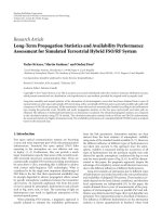
Figure 1: DOA estimates RMSE of the proposed EVSA-PM against SNRs. (a) Source 1, (b) source 2.
matching the eigenvectors of the different matrices P
†
1
P
2n−1
(n = 2, ,6) [11]. With the estimated c(θ
k
, ϕ
k
, γ
k
, η
k
) =
[1,
d
2,k
, ,
d
6,k
]
T
, the Poynting vector estimates can be
obtained by the vector cross-product operation and then the
DOA and polarization parameters are estimated from the
normalized Poynting vectors [11]. For a dipole triad array or
loop triad array, the estimates of the electric field vector e
k
or
the magnetic field vector h
k
canbedoneinthesameway.In
this case, the DOA and polarization parameter estimates can
be obtained using the amplitude-normalized estimates of the
electric or magnetic field steering vector [3].
In order to calculate the propagator matrix P,wedivide
the matrix R
e
into R
e
= [R
T
e1
, R
T
e2
]
T
,whereR
e1
and R
e2
consist of the first K rows and the last 6L − 6 − K rows of
R
e
. In the noise-free case, we have P
H
R
e1
= R
e2
.Inthenoise
case, a least squares solution can be used to estimate P
P =
R
e1
R
H
e1
−1
R
e1
R
H
e2
. (23)
3.3. EVSA-PM Algorithm for Estimating Par ameters by Angle
Searching. The EVSA-PM is also applied to the uniform
linear array comprising any types of identical EmVSs. In the
case, the estimates of DOA and polarization parameters can-
not be extracted from the estimates of the steering vectors.
However, they are obtainable by the use of parameter-space
searching techniques. We here use two-dimensional angle
searching to estimate the DOA.
Consider N-component EmVS array (2
≤ N ≤ 6),
then the matrix A
e
in (15)canberewrittenasA
e
= [A
T
e,1
,
, A
T
e,N
]
T
∈ C
N(L−1)×K
,andA
e,n
can also be rewritten as
A
e,n
= Q
e
n
, n = 1, , N, (24)
where Q
e
def
= [q
e
(θ
1
, ϕ
1
), , q
e
(θ
K
, ϕ
K
)] ∈ C
(L−1)×K
,
n
def
=
diag(c
n,1
, , c
n,K
) ∈ C
K×K
.
Defining g
n
def
=
[0
L−1,(L−1)(n−1)
, I
L−1
, 0
L−1,(L−1)(N−n)
] ∈
R
(L−1)×N(L−1)
,wehaveR
g
def
=
N
n
=1
g
n
R
e
= Q
e
ΠΩ,where
Π
def
=
N
n
=1
Π
n
. Partitioning R
g
into R
g
= [ R
T
g1
R
T
g2
]
T
,where
R
g1
and R
g2
consist o f the first K rows and the last L −
1 − K rows of R
g
,wehavethepropagatormatrixP =
(R
g1
R
H
g1
)
−1
R
g1
R
H
g2
. Then the source’s DOA parameters can be
estimated as
θ
k
, ϕ
k
=
arg min
{
θ,ϕ
}
q
H
e
θ, ϕ
ΨΨ
H
q
e
θ, ϕ
, (25)
where Ψ
def
= [P
T
, −I
L−1−K
]
T
.
4. Simulations
We conduct computer simulations to evaluate the perfor-
mances of the proposed EVSA-PM. Comparison with the
PSA based [19] PM (PSA-PM) and the SUMWE algorithm
[26] is also made. For proposed EVSA-PM algorithm, the
parameter estimates shown in Figures 1–5 are extracted from
the EmVS steering vector, and those shown in Figure 6 are
obtained by angle searching. The performance metrics used
is the root mean square errors (RMSEs) of the sources’ 2-D
DOA and the polarization parameters estimates, where the
RMSE of kth source’s 2-D DOA estimate is defined as
RMSE
k
=
1
2
⎧
⎪
⎨
⎪
⎩
1
E
⎛
⎝
E
e=1
θ
e,k
− θ
k
2
⎞
⎠
+
1
E
⎛
⎝
E
e=1
ϕ
e,k
− ϕ
k
2
⎞
⎠
⎫
⎪
⎬
⎪
⎭
,
(26)
6 EURASIP Journal on Advances in Signal Pr ocessing
−10
0
10 20
30
40
10
−3
10
−2
10
−1
10
0
10
1
10
2
SNR (dB)
0.5λ
2λ
4λ
8λ
10
3
Polar RMSE (deg)
(a)
−10
0102030
40
10
−3
10
−2
10
−1
10
0
10
1
10
2
SNR (dB)
0.5λ
2λ
4λ
8λ
Polar RMSE (deg)
(b)
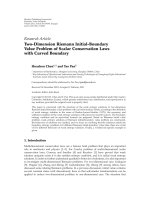
Figure 2: Polarization state estimates RMSE of the proposed EVSA-PM against SNRs. (a) Source 1, (b) source 2.
PSA-PM
SUMWE
CRB
−10
0
10 20
30
40
10
−3
10
−2
10
−1
10
0
10
1
10
2
SNR (dB)
DOA RMSE (deg)
EVSA-PM (Δ = 4λ)
EVSA-PM (Δ
= λ/2)
(a)
PSA-PM
SUMWE
CRB
−10
0
10 20
30
40
10
−3
10
−2
10
−1
10
0
10
1
10
2
SNR (dB)
DOA RMSE (deg)
EVSA-PM (Δ = 4λ)
EVSA-PM (Δ
= λ/2)
(b)
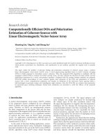
Figure 3: DOA estimate RMSEs of EVSA-PM, PSA-PM, and SUMWE against SNRs. (a) Source 1, (b) source 2.
and the RMSE of kth source’s polarization state estimate is
defined as
RMSE
k
=
1
2
⎧
⎪
⎨
⎪
⎩
1
E
⎛
⎝
E
e=1
γ
e,k
− γ
k
2
⎞
⎠
+
1
E
⎛
⎝
E
e=1
η
e,k
− η
k
2
⎞
⎠
⎫
⎪
⎬
⎪
⎭
,
(27)
where
θ
e,k
, ϕ
e,k
, γ
e,k
,andη
e,k
symbolize the eth Monte
Carlo trial’s estimates for the kth source’s directions and
polarization states and E is the total Monte Carlo trials. In
the simulations, E
= 500.
Figures 1 and 2 plot the RMSEs of the sources’ DOA and
polarization estimates against signal-to-noise ratio (SNR)
levels using the EVSA-PM. The SNR is defined as SNR
=
(1/K)
K
k
=1
|s
k
|
2
/σ
2
n
,whereσ
2
n
is the noise power lever . Two
equal-power narrowband coherent signals impinge with
parameters θ
1
= 75
◦
, ϕ
1
= 35
◦
, γ
1
= 45
◦
, η
1
=−90
◦
, θ
2
=
80
◦
, ϕ
2
= 30
◦
, γ
2
= 45
◦
,andη
2
= 90
◦
, and the multipath
coefficient is set to β
2
= exp( j ∗ 50
◦
). The uniform linear
array consists of 12 six-component EmVSs. The intervector
sensor spacing is set as Δ
=
Δ
2
x
+ Δ
2
y
= 0.5λ,2λ,4λ,and
8λ, respectively. The snapshot number is 300. It is seen from
that both DOA and polarization estimation errors decreases
as the SNR increases. Also, the inc rease of intervector
sensor spacing, which results in the array aperture extension,
EURASIP Journal on Advances in Sig nal Processing 7
EVSA-PM (Δ = 4λ)
EVSA-PM (Δ
= λ/2)
PSA-PM
SUMWE
CRB
10
1
10
2
10
3
Snapshot number
10
−2
10
−1
10
0
10
1
10
2
DOA RMSE (deg)
(a)
EVSA-PM (Δ = 4λ)
EVSA-PM (Δ
= λ/2)
PSA-PM
SUMWE
CRB
10
1
10
2
10
3
Snapshot number
10
−2
10
−1
10
0
10
1
10
2
DOA RMSE (deg)
(b)
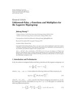
Figure 4: DOA estimate RMSEs of EVSA-PM, PSA-PM and SUMWE against the number of snapshots. (a) Source 1, (b) source 2.
65
66 67 68 69 70 71 72 73 74
75
0
10
20
30
40
50
60
70
Elevation angle
EVSA-PM
(a)
65 66 67 68 69 70 71 72 73 74 75
0
10
20
30
40
50
60
Elevation angle
PSA-PM
(b)
65 66 67 68 69 70 71 72 73 74 75
Elevation angle
SUMWE
0
5
10
15
20
25
30
(c)
Figure 5: The histogram of the estimated elevation using the three methods. (a) EVSA-PM; (b) PSA-PM; (c) SUMWE.
8 EURASIP Journal on Advances in Signal Pr ocessing
contributes to the estimation accuracy enhancement. Since
the estimation of DOA and polarization is extracted from
the EmVS steering vector, which contains no time-delay
phase factor, we can obtain more accurate but unambiguous
estimates of coherent source using an aperture extension
array without a corresponding increase in hardware and
software costs [12].
Figures 3 and 4 make the comparison between the
proposed algorithm with PSA-PM and SUMWE under
different SNRs and number of snapshots. The impinging
signal parameters are same as in Figures 1 and 2.Weuse
300 snapshots in Figure 3 and set SNR
= 20 dB in Figure 4.
For the proposed algorithm, a uniform linear array w ith 8
dipole-triads, separated by Δ
= λ/2and4λ is considered.
For the PSA-PM, we use an L-shape geometry, with 8 dipole-
triads uniformly placed along x-axis for estimating u
k
and
8 dipole-triads uniformly placed along y-axis for estimating
v
k
. For the SUMWE, we use an L-shape geometry, with
12 unpolarized scalar sensors uniformly placed along x-
axis for estimating u
k
and 12 unpolarized scalar sensors
uniformly placed along y-axis for estimating v
k
.Hence,the
hardware costs of the SUMWE and the presented algorithm
are comparable. The intersensor displacement for the PSA-
PM and SUMWE is a half-wavelength, since these two
algorithms would suffer angle ambiguities when two sensors
are spaced over a half-wavelength. The curves in these two
figures unanimously demonstrate that the proposed EVSA-
PM with Δ
= 4λ can offer performance superior to those of
the PSA-PM and SUMWE.
From the computational complexity analysis, the major
computational costs involved in the three algorithms are the
calculation of the corresponding propagator and correlation
matrix, and the numbers of multiplications required by the
EVSA-PM, the PSA-PM, and SUMWE are in the order of
O(3M
1
KF + 18(M
1
− 1)F) ≈ 174F, O(2M
1
KF +6M
2
1
F) ≈
416F,andO(2M
2
KF +4(M
2
− 1)F) ≈ 92F, respectively,
where M
1
= 8, M
2
= 12, and F denotes the number of
snapshots. Therefore, the proposed EV SA-PM also is more
computationally efficient than the PSA-PM.
The proposed EVSA-PM can fully exploit polarization
diversity to resolve closely spaced sources with distinct
polarizations. To verify this performance, we assume two
incident coherent sources with parameters θ
1
= 70
◦
, θ
2
=
70.5
◦
, ϕ
1
= 90
◦
, ϕ
2
= 90
◦
, γ
1
= 45
◦
, γ
2
= 45
◦
, η
1
=−90
◦
,
and η
2
= 90
◦
. Others simulation conditions are the same as
that in Figure 4,exceptthattheSNRissetat35dB.Figure 5
shows the histogram of the estimated elevation using the
three methods based on 500 independent trials. From the
figure, we can observe that the proposed EVSA-PM can
resolve the closely spaced sources. However, the other two
methods fail.
Figure 6 plots the spatial spectrum to present comparison
of the maximum numbers of coherent signals, which can
be, respectively, resolved by the proposed algorithm, the
SUMWE, the PSA-PM, and the PSA-FB-PM which combines
the PSA with the FB averaging technique [27]. We consider
a uniform linear array comprised of 20 unpolarized scalar
sensors for the SUMWE and 20 quadrature polarized vector
0 20 40 60 80 100 120 140 160 180
−40
−20
0
20
40
60
80
100
120
DOA (deg)
Spatial spectrum (dB)
EVSA-PM
PSA-PM
PSA-FB-PM
SUMWE
Figure 6: Spatial spectrum of EVSA-PM, PSA-PM, PSA-FB-PM,
and SUMWE for nine coherent sources.
sensors [19](i.e.,N = 4, M = 20) for all the other
three algorithms and estimate the sources’ direction by angle
searching. The intervector sensor spacing of array is a half-
wavelength. Like [19], we assume zero elevation incident
angle (θ
k
= 90
◦
) and randomly chosen polarizations for all
sources, and set SNR
= 15 dB.
Nine equal power, coherent sources with the azimuth
incident angles 35
◦
,50
◦
,65
◦
,80
◦
,90
◦
, 100
◦
, 110
◦
, 125
◦
,
and 140
◦
are considered, and the corresponding multipath
coefficients β
k
= exp( j ∗ 10
◦
(k − 1)), k = 1, ,9. This
figure shows that the proposed EVSA-PM and the SUMWE
successfully resolve the nine coherent signals, while the PSA-
PM, and the PSA-FB-PM fail to do so. This is due to the
factor that the PSA-PM and the PSA-FB-PM, respectively,
only can resolve min(N , M
− 1) = 4 and min(2N, M − 1) = 8
coherent sources at most, while the proposed EVSA-PM can
resolve L
− 2 coherent sources (L = M − K +1),andthe
maximum number of coherent signals resolved using t he
SUMWEisequaltothatusingtheEVSA-PM.
5. Conclusions
This paper employs a linear electromagnetic vector-sensor
array to propose a novel pre-processing algorithm for
decorrelating the coherent signals by electromagnetic vector-
sensor subarray averaging, and combine it with the propaga-
tor method to estimate the DOA and polarization of coher-
ent sources without eigen-decomposition into signal/noise
subspaces. Compared with the existing estimate algorithms,
the proposed algorithm makes use of more available electro-
magnetic information, henc e, has an impro ved estimation
performance. It does not necessarily require the intervector
sensor spacing of a half-wavelength, enable decorrelation of
more coherent signals, and joint estimation of DOA and
polarization of coherent sources.
EURASIP Journal on Advances in Sig nal Processing 9
Appendix
From (12), we can obtain
[
R
1
, , R
6
]
def
=
AFG,(A.1)
where F
def
= diag (r
s
1
β
1
, ,r
s
1
β
K
1
,r
s
K
1
+1
q
M
(θ
K
1
+1
, ϕ
K
1
+1
), ,
r
s
K
q
M
(θ
K
, ϕ
K
))
G
def
=
⎡
⎢
⎢
⎢
⎢
⎢
⎢
⎢
⎢
⎢
⎢
⎢
⎢
⎢
⎢
⎢
⎢
⎣
ρ
M,1
h
T
1
ρ
M,2
h
T
1
ρ
M,6
h
T
1
.
.
.
.
.
.
.
.
.
.
.
.
ρ
M,1
h
T
K
1
ρ
M,2
h
T
K
1
ρ
M,6
h
T
K
1
c
1,K
1
+1
h
T
K
1
+1
c
2,K
1
+1
h
T
K
1
+1
c
6,K
1
+1
h
T
K
1
+1
.
.
.
.
.
.
.
.
.
.
.
.
c
1,K
h
T
K
c
2,K
h
T
K
c
6,K
h
T
K
⎤
⎥
⎥
⎥
⎥
⎥
⎥
⎥
⎥
⎥
⎥
⎥
⎥
⎥
⎥
⎥
⎥
⎦
h
k
def
=
q
1
θ
k
, ϕ
k
, ,q
K
θ
k
, ϕ
k
T
.
,
(A.2)
The m atrix
A is of full column rank due to the distinct
polarizations (although there are two sources from the same
direction). The diagonal matrix F has full rank. If the two
sources have the same incident directions but with the
distinct polarizations, and are uncorrelated w ith each other
(i.e., the two sources are not all included in t he set consisting
of the first K
1
coherent sources), the K ×6K matrix G is of full
row rank. Therefore, in this scenario, the matrix [R
1
, , R
6
]
is of rank K. Similarly, the matrix [
R
1
, ,
R
6
]alsoisofrank
K.Thus,thematrixR defined in (11)stillhasfullrank.
References
[1] A. Nehorai and E. Paldi, “Vector-sensor array processing for
electromagnetic source localization,” IEEE Tr ansactions on
Signal Processing, vol. 42, no. 2, pp. 376–398, 1994.
[2] J. Li, “Direction and polarization estimation using arrays with
small loops and short dipoles,” IEEE Transactions on Antennas
and Propagation, vol. 41, no. 3, pp. 379–386, 1993.
[3] K. T. Wong, “Direction finding/polarization estimation—
dipole and/or loop triad(s),” IEEE Transactions on Aerospace
and Electronic Systems, vol. 37, no. 2, pp. 679–684, 2001.
[4] B. Hochwald and A. Nehorai, “Polarimetric modeling and
parameter estimation with applications to remote sensing,”
IEEE Transactions on Signal Processing, vol. 43, no. 8, pp. 1923–
1935, 1995.
[5]X.Gong,Z.Liu,Y.Xu,andM.IshtiaqAhmad,“Direction-
of-arrival estimation via twofold mode-projection,” Sig nal
Processing, vol. 89, no. 5, pp. 831–842, 2009.
[6] J. Tabrikian, R. Shavit, and D. Rahamim, “An efficient vector
sensor configuration for source localization,” I EEE Signal
Processing Letters, vol. 11, no. 8, pp. 690–693, 2004.
[7] S.Miron,N.LeBihan,andJ.I.Mars,“Quaternion-MUSICfor
vector-sensor array processing,” IEEE Transactions on Signal
Processing, vol. 54, no. 4, pp. 1218–1229, 2006.
[8] C. C. Ko, J. Zhang, and A. Nehorai, “Separation and tracking
of multiple broadband sources with one electromagnetic
vector sensor,” IEEE Transactions on Aerospace and Electronic
Systems, vol. 38, no. 3, pp. 1109–1116, 2002.
[9] C. Paulus and J. I. Mars, “Vector-sensor array processing
for polarization parameters and DOA estimation,” EURASIP
Journal on Advances in Signal Processing, vol. 2010, Article ID
850265, 3 pages, 2010.
[10] Y.Xu,Z.Liu,K.T.Wong,andJ.Cao,“Virtual-manifoldambi-
guity in HOS-based direction-finding with electromagnetic
vector-sensors,” I EEE Tr ansactions o n Aerospace and Electronic
Systems, vol. 44, no. 4, pp. 1291–1308, 2008.
[11] K. T. Wong and M. D. Zoltowski, “Closed-form direction
finding and polarization estimation w ith arbitrarily spaced
electromagnetic vector-sensors at unknown locations,” IEEE
Transactions on Antennas and Propagation, vol. 48, no. 5,
pp. 671–681, 2000.
[12] M. D. Zoltowski and K. T. Wong, “ESPRIT-based 2-D direc-
tion finding with a sparse uniform array of electromagnetic
vector sensors,” IEEE Transactions on Signal Processing, vol. 48,
no. 8, pp. 2195–2204, 2000.
[13] K. T. Wong, “Blind beamforming geolocation for wideband-
FFHs with unknown hop-sequences,” IEEE Transactions on
Aerospace and Electronic Systems, vol. 37, no. 1, pp. 65–76,
2001.
[14] H. Jiacai, S . Yaowu, and T. Jianwu, “Joint estimation of DOA,
frequency, and polarization based on cumulants and UCA,”
Journal of Systems Engineering and Electronics, vol. 18, no. 4,
pp. 704–709, 2007.
[15]K.C.Ho,K.C.Tan,andA.Nehorai,“Estimatingdirec-
tions of ar r ival of completely and incompletely polarized
signals with electromagnetic vector sensors,” IEEE Transac-
tions on Signal Processing, vol. 47, no. 10, pp. 2845–2852,
1999.
[16] K. T. Wong and M. D. Zoltowski, “Uni-vector-sensor ESPRIT
for multisource azimuth, elevation, and polarization estima-
tion,” IEEE Transactions on Antennas and Propagation, vol. 45,
no. 10, pp. 1467–1474, 1997.
[17]K.T.WongandM.D.Zoltowski,“Self-initiatingMUSIC-
based direction finding and polarization estimation in spatio-
polarizational beamspace,” IEEE Transactions on Antennas and
Propagation, vol. 48, no. 8, pp. 1235–1245, 2000.
[18] M. D. Zoltowski and K. T. Wong, “Closed-form eigenstruc-
ture-based direction finding using arbitrary but identical
subarrays on a sparse uniform Cartesian array grid,” IEEE
Transactions on Signal Processing, vol. 48, no. 8, pp. 2205–2210,
2000.
[19] D. Rahamim, J. Tabrikian, and R. Shavit, “Source localization
using vector sensor array in a multipath environment,” IEEE
Transactions on Signal Processing, vol. 52, no. 11, pp. 3096–
3103, 2004.
[20]Y.Wu,H.C.So,C.Hou,andJ.Li,“Passivelocalizationof
near-field sources with a polarization sensitive array,” IEEE
Transactions on Antennas and Propagation, vol. 55, no. 8,
pp. 2402–2408, 2007.
[21] M. K anda and D. A. Hill, “A three-loop method for deter-
mining the radiation characteristics of an electrically small
source,” IEEE Transactions on Electromagnetic Compatibility,
vol. 34, no. 1, pp. 1–3, 1992.
[22] R. O. Schmidt, “Multiple emitter location and signal param-
eter estimation,” IEEE Transactions on Antennas and Propaga-
tion, vol. 34, no. 3, pp. 276–280, 1986.
[23] R. Roy and T. Kailath, “ESPRIT—estimation of signal parame-
ters via rotational invariance techniques,” IEEE Transactions on
Acoustics, Speech, and Signal Processing, vol. 37, no. 7, pp. 984–
995, 1989.
10 EURASIP Journal on Advances in Signal Processing
[24] N. Tayem and H. M. Kwon, “L-shape 2-dimensional arrival
angle estimation with propagator method,” IEEE Transactions
on Antennas and Propagation, vol. 53, no. 5, pp. 1622–1630,
2005.
[25] C.Gu,J.He,X.Zhu,andZ.Liu,“Efficient 2D DOA estimation
of coherent signals in spatially c orrelated n oise using electro-
magnetic vector sensors,” Multidimensional Systems and Signal
Processing, vol. 21, no. 3, pp. 239–254, 2010.
[26] J. Xin and A. Sano, “Computationally efficient subspace-
based m ethod for direction-of-arrival estimation without
eigendecomposition,” IEEE Transactions on Signal Processing,
vol. 52, no. 4, pp. 876–893, 2004.
[27] S. U. Pillai and B. H. Kwon, “Forward/backward spatial
smoothing techniques for coherent signal identification,” IEEE
Transactions on Acoustics, Speech, and Signal Processing, vol. 37,
no. 1, pp. 8–15, 1989.