Báo cáo hóa học: " Research Article On Efficient Method for System of Fractional Differential Equations" potx
Bạn đang xem bản rút gọn của tài liệu. Xem và tải ngay bản đầy đủ của tài liệu tại đây (832.54 KB, 15 trang )
Hindawi Publishing Corporation
Advances in Difference Equations
Volume 2011, Article ID 303472, 15 pages
doi:10.1155/2011/303472
Research Article
On Efficient Method for System of
Fractional Differential Equations
Najeeb Alam Khan,
1
Muhammad Jamil,
2, 3
Asmat Ara,
1
and Nasir-Uddin Khan
1
1
Department of Mathematics, University of Karachi, Karachi 75270, Pakistan
2
Abdul Salam School of Mathematical Sciences, GC University, Lahore, Pakistan
3
Department of Mathematics, NEDUET, Karachi 75270, Pakistan
Correspondence should be addressed to Najeeb Alam Khan,
Received 14 December 2010; Accepted 5 February 2011
Academic Editor: J. J. Trujillo
Copyright q 2011 Najeeb Alam Khan et al. This is an open access article distributed under the
Creative Commons Attribution License, which permits unrestricted use, distribution, and
reproduction in any medium, provided the original work is properly cited.
The present study introduces a new version of homotopy perturbation method for the solution
of system of fractional-order differential equations. In this approach, the solution is considered as
a Taylor series expansion that converges rapidly to the nonlinear problem. The systems include
fractional-order stiff system, the fractional-order Genesio system, and the fractional-order matrix
Riccati-type differential equation. The new approximate analytical procedure depends only on two
components. Comparing the methodology with some known techniques shows that the present
method is relatively easy, less computational, and highly accurate.
1. Introduction
Fractional differential equations have received considerable interest in recent years and
have been extensively investigated and applied for many real problems which are modeled
in different areas. One possible explanation of such unpopularity could be that there are
multiple nonequivalent definitions of fractional derivatives 1.Anotherdifficulty is that
fractional derivatives have no evident geometrical interpretation because of their nonlocal
character. However, during the last 12 years fractional calculus starts to attract much more
attention of scientists. It was found that various, especially interdisciplinary, applications 2–
6 can be elegantly modeled with the help of the fractional derivatives.
The homotopy perturbation method is a powerful devise for solving nonlinear
problems. This method was introduced by He 7–9 in the year 1998. In this method,
the solution is considered as the summation of an infinite series that converges rapidly.
2AdvancesinDifference Equations
This technique is used for solving nonlinear chemical engineering equations 10,time-
fractional Swift-Hohenberg S-H equation 11, viscous fluid flow equation 12,Fourth-
Order Integro-Differential equations 13, nonlinear dispersive Km, n, 1 equations 14,
Long Porous Slider equation 15, and Navier-Stokes equations 16. It can be said that He’s
homotopy perturbation method is a universal one, which is able to solve various kinds of
nonlinear equations. The new homotopy perturbation method NHPM was applied to linear
and nonlinear ODEs 17.
In this paper, we construct the solution of system of fractional-order differential
equations by extending the idea of 17, 18. This method leads to computable and efficient
solutions to linear and nonlinear operator equations. The corresponding solutions of the
integer-order equations are found to follow as special cases of those of fractional-order
equations.
We consider the system of fractional-order equations of the form
D
α
i
y
i
t
F
i
t, y
1
,y
2
,y
3
, ,y
n
f
i
t
,y
i
t
0
c
i
, 0 <α
i
≤ 1,i 1, 2, ,n. 1.1
2. Basic Definitions
We give some basic definitions, notations, and properties of the fractional calculus theory
used in this work.
Definition 2.1. The Riemann-Liouville fractional integral operator J
μ
of order μ on the usual
Lebesgue space L
1
a, b is given by
J
μ
f
x
1
Γ
μ
x
0
x − t
μ−1
f
t
dt, μ > 0,
J
0
f
x
f
x
.
2.1
It has the following properties:
i J
μ
exists for any x ∈ a, b,
ii J
μ
J
β
J
μβ
,
iii J
μ
J
β
J
β
J
μ
,
iv J
α
J
β
fxJ
β
J
α
fx,
v J
μ
x − a
γ
Γγ 1/Γα γ 1x − a
μγ
,
where f ∈ L
1
a, b, μ, β ≥ 0andγ>−1.
Definition 2.2. The Caputo definition of fractal derivative operator is given by
D
μ
f
x
J
m−μ
D
n
f
x
1
Γ
m − μ
t
0
x − τ
m−μ−1
f
m
τ
dτ, 2.2
Advances in Difference Equations 3
where m − 1 <μ≤ m, m ∈ N, x > 0. It has the following two basic properties for m − 1 <
μ ≤ m and f ∈ L
1
a, b:
D
μ
J
μ
f
x
f
x
,
J
μ
D
μ
f
x
f
x
−
m−1
k0
f
k
0
x − a
k
k!
,x>0.
2.3
3. Analysis of New Homotopy Perturbation Method
Let us consider the system of nonlinear differential equations
A
i
y
i
f
i
t
,t∈ Ω, 3.1
where A
i
are the operators, f
i
are known functions and y
i
are sought functions. Assume that
operators A
i
canbewrittenas
A
i
y
i
L
i
y
i
N
i
y
i
, 3.2
where L
i
are the linear operators and N
i
are the nonlinear operators. Hence, 3.1 can be
rewritten as follows:
L
i
y
i
N
i
y
i
f
i
t
,t∈ Ω. 3.3
We define the operators H
i
as
H
i
Y
i
; p
≡
1 − p
L
i
Y
i
−L
i
y
i,0
p
A
i
Y
− f
i
, 3.4
where p ∈ 0, 1 is an embedding or homotopy parameter, Y
i
t; p : Ω × 0, 1 → and y
i,0
are the initial approximation of solution of the problem in 3.3 can be written as
H
i
Y
i
; p
≡L
i
Y
i
−L
i
y
i,0
pL
i
y
i,0
p
N
i
Y
i
− f
i
. 3.5
Clearly, the operator equations H
i
v, 00andH
i
v, 10 are equivalent to the equations
L
i
Y
i
−Ly
i,0
0andA
i
Y − f
i
t0, respectively. Thus, a monotonous change of
parameter p from zero to one corresponds to a continuous change of the trivial problem
L
i
Y
i
−L
i
y
i,0
0 to the original problem. Operator H
i
Y
i
,p is called a homotopy map.
Next, we assume that the solution of equation H
i
Y
i
,p canbewrittenasapowerseriesin
embedding parameter p, as follows:
Y
i
Y
i,0
pY
i,1
,i 1, 2, 3, ,n. 3.6
Now, let us write 3.5 in the following form:
L
i
Y
i
y
i,0
t
p
f
i
−N
i
Y
i
− y
i,0
t
. 3.7
4AdvancesinDifference Equations
By applying the inverse operator, L
−1
i
to both sides of 3.7,wehave
Y
i
L
−1
i
y
i,0
t
p
L
−1
i
f −L
−1
i
N
i
Y
i
−L
−1
i
y
i,0
t
. 3.8
Suppose that the initial approximation of 3.3 has the form
y
i,0
t
∞
n0
a
i,n
P
n
t
,i 1, 2, 3, ,n, 3.9
where a
i,n
, n 0, 1, 2, are unknown coefficients and P
n
t, n 0, 1, 2, are specific
functions on the problem. By substituting 3.6 and 3.9 into 3.8,weget
Y
i,0
pY
i,1
L
−1
i
∞
n0
a
i,n
P
n
t
p
L
−1
i
f
i
−L
−1
i
N
i
Y
i,0
pY
i,1
−L
−1
i
∞
n0
a
i,n
P
n
t
.
3.10
Equating the coefficients of like powers of p, we get the following set of equations:
coefficient of p
0
: Y
0
L
−1
∞
n0
a
i,n
P
n
t
,
coefficient of p
1
: Y
1
L
−1
i
f
i
L
−1
i
Y
i,1
−L
−1
i
N
i
Y
i,0
.
3.11
Now, we solve these equations in such a way that Y
i,1
t0. Therefore, the approximate
solution may be obtained as
y
i
t
Y
i,0
t
L
−1
∞
n0
a
i,n
P
n
t
. 3.12
4. Applications
Application 1
Consider the following linear fractional-order 2-by-2 stiff system:
D
α
t
u
t
k
−1 − ε
u
t
k
1 − ε
v
t
,
D
α
t
v
t
k
1 − ε
u
t
k
−1 − ε
v
t
4.1
with the initial conditions
u
0
1,v
0
3, 4.2
Advances in Difference Equations 5
where k and ε are constants. To obtain the solution of 4.1 by NHPM, we construct the
following homotopy:
1 − p
D
α
t
U
t
− u
0
t
p
D
α
t
U
t
− k
−1 − ε
U
t
− k
1 − ε
V
t
0,
1 − p
D
α
t
V
t
− v
0
t
p
D
α
t
V
t
− k
1 − ε
U
t
− k
−1 − ε
V
t
0.
4.3
Applying the inverse operator, J
α
t
of D
α
t
both sides of the above equation, we obtain
U
t
U
0
J
α
t
u
0
t
− pJ
α
t
u
0
t
− k
−1 −ε
U
t
− k
1 − ε
V
t
,
V
t
V
0
J
α
t
v
0
t
− pJ
α
t
v
0
t
− k
1 − ε
U
t
− k
−1 − ε
V
t
.
4.4
The solution of 4.1 to has the following form:
U
t
U
0
t
pU
1
t
,V
t
V
0
t
pV
1
t
. 4.5
Substituting 4.5 in 4.4 and equating the coefficients of like powers of p,wegetthe
following set of equations:
U
0
t
U
0
J
α
t
u
0
t
,V
0
t
V
0
J
α
t
v
0
t
,
U
1
t
J
α
t
−u
0
t
k
−1 − ε
U
0
t
k
1 − ε
V
0
t
,
V
1
t
J
α
t
−v
0
t
k
1 − ε
U
0
t
k
−1 −ε
V
0
t
.
4.6
Assuming u
0
t
20
n0
a
n
P
n
, v
0
t
20
n0
b
n
P
n
, P
k
t
k
, U0u0,andV 0v0 and
solving the above equation for U
1
t and V
1
t lead to the result
U
1
t
2k − 4εk − a
0
t
α
Γ
α 1
−
a
1
t
α1
Γ
α 2
−
2a
2
t
α2
Γ
α 3
−
6a
3
t
α3
Γ
α 4
−
24a
4
t
2α
Γ
α 5
···,
V
1
t
−2k − 4εk − b
0
t
α
Γ
α 1
−
b
1
t
α1
Γ
α 2
−
2b
2
t
α2
Γ
α 3
−
6b
3
t
α3
Γ
α 4
−
24b
4
t
2α
Γ
α 5
···.
4.7
Vanishing U
1
t and V
1
t lets the coefficients a
i
,b
i
,i 0, 1, 2, by taking α 1 the following
values:
a
0
2k
1 − 2ε
,a
1
−4k
2
1 − 2ε
2
,a
2
4k
3
1 − 2ε
3
,
a
3
−8k
4
1 − 2ε
4
3
,a
4
4k
5
1 − 2ε
5
3
,a
5
−8k
6
1 − 2ε
6
15
,
a
6
8k
7
1 − 2ε
7
45
,a
7
−16k
8
1 − 2ε
8
315
,a
8
4k
9
1 − 2ε
9
315
,
a
9
−8k
10
1 − 2ε
10
2835
,a
10
8k
11
1 − 2ε
11
14175
,a
11
−16k
12
1 − 2ε
12
155925
,
6AdvancesinDifference Equations
a
12
8k
13
1 − 2ε
13
467775
,a
13
−16k
14
1 − 2ε
14
6081075
,a
14
16k
15
1 − 2ε
15
42567525
,
a
15
−16k
16
1 − 2ε
16
155925
,a
16
4k
17
1 − 2ε
17
638512875
,a
17
−8k
18
1 − 2ε
18
10854718875
,
a
18
8k
19
1 − 2ε
19
97692469875
,a
19
−16k
20
1 − 2ε
20
1856156927625
,a
20
8k
21
1 − 2ε
21
9280784638125
,
b
0
−2k
1 2ε
,b
1
4k
2
1 2ε
2
,b
2
−4k
3
1 2ε
3
,
b
3
8k
4
1 2ε
4
3
,b
4
−4k
5
1 2ε
5
3
,b
5
8k
6
1 2ε
6
15
,
b
6
−8k
7
1 2ε
7
45
,b
7
16k
8
1 2ε
8
315
,b
8
−4k
9
1 2ε
9
315
,
b
9
8k
10
1 2ε
10
2835
,b
10
−8k
11
1 2ε
11
14175
,b
11
16k
12
1 2ε
12
155925
,
b
12
−8k
13
1 2ε
13
467775
,b
13
16k
14
1 2ε
14
6081075
,b
14
−16k
15
1 2ε
15
42567525
,
b
15
16k
16
1 2ε
16
155925
,b
16
−4k
17
1 2ε
17
638512875
,b
17
8k
18
1 2ε
18
10854718875
,
b
18
−8k
19
1 2ε
19
97692469875
,b
19
16k
20
1 2ε
20
1856156927625
,b
20
−8k
21
1 2ε
21
9280784638125
.
4.8
Therefore, we obtain the solutions of 4.1 as
u
t
1
2k
1 − 2ε
t
α
Γ
α 1
−
4k
2
1 − 2ε
2
t
α1
Γ
α 2
8k
3
1 − 2ε
3
t
α2
Γ
α 3
−
16k
4
1 − 2ε
4
t
α3
Γ
α 4
···,
v
t
3 −
2k
1 2ε
t
α
Γ
α 1
4k
2
1 2ε
2
t
α1
Γ
α 2
−
8k
3
1 2ε
3
t
α2
Γ
α 3
−
16k
4
1 2ε
4
t
α3
Γ
α 4
···.
4.9
Our aim is to study the mathematical behavior of the solution ut and vt for different
values of α. This goal can be achieved by forming Pade’ approximants, which have the
advantage of manipulating the polynomial approximation into a rational function to gain
more information about ut and vt. It is well known that Pade’ approximants will converge
ontheentirerealaxis,ifut and vt are free of singularities on the real axis. It is of interest to
note that Pade’ approximants give results with no greater error bounds than approximation
by polynomials. To consider the behavior of solution for different values of α, we will take
advantage of the explicit formula 4.9 available for 0 <α≤ 1 and consider the following two
special cases.
Advances in Difference Equations 7
Case 1. Setting α 1,k 50,ε 0.01 in 4.9, we obtain the approximate solution in a series
form as
u
10,11
t
1 148.73t 1203.65t
2
51963.1t
3
···
1 50.7628t 1227.89t
2
18726.5t
3
···
,
v
10,11
t
3 69.439t 3823.59t
2
40311.9t
3
···
1 57.1463t 1550.5t
2
26447.2t
3
···
.
4.10
Case 2. In this case, we will examine the linear fractional stiff equation 4.1. Setting α
1/2,k 50,ε 0.01 in 4.9 gives
u
t
1
196t
1/2
√
π
−
39992t
3/2
3
√
π
7999984t
5/2
15
√
π
−
228571424t
7/2
15
√
π
···,
v
t
3 −
204t
1/2
√
π
13336t
3/2
√
π
−
2666672t
5/2
5
√
π
533333344t
7/2
35
√
π
−···.
4.11
For simplicity, let t
1/2
z,then
u
z
1
196z
√
π
−
39992z
3
3
√
π
7999984z
5
15
√
π
−
228571424z
7
15
√
π
···,
v
z
3 −
204z
√
π
13336z
3
√
π
−
2666672z
5
5
√
π
533333344z
7
35
√
π
−···.
4.12
Calculating the 10/11 Pade’ approximants and recalling that z t
1/2
,weget
u
10,11
9.58 × 10
−8
0.0000126t
1/2
0.0002357t − 0.0001051t
3/2
−···
9.581 ×10
−8
2.0904 × 10
−6
t
1/2
4.56399 ×10
−6
t 0.000096t
2
···
,
v
10,11
2.66 ×10
123
− 1.216 × 10
125
t
1/2
8.69947 ×10
125
t ···
8.88 × 10
122
− 6.45605 ×10
123
t
1/2
4.22967 ×10
124
t ···
.
4.13
Application 2
Consider the following nonlinear fractional-order 2-by-2 stiff system:
D
α
t
u
t
−1002u
t
1000v
2
t
,
D
α
t
v
t
u
t
− v
t
− v
2
t
4.14
with the initial conditions
u
0
1,v
0
1. 4.15
8AdvancesinDifference Equations
To obtain the solution of 4.14 by NHPM, we construct the following homotopy:
1 − p
D
α
t
U
t
− u
0
t
p
D
α
t
U
t
1002U
t
− 1000V
2
t
0,
1 − p
D
α
t
V
t
− v
0
t
p
D
α
t
V
t
− U
t
V
t
V
2
t
0.
4.16
Applying the inverse operator, J
α
t
of D
α
t
both sides of the above equation, we obtain
U
t
U
0
J
α
t
u
0
t
− pJ
α
t
u
0
t
1002U
t
− 1000V
2
t
,
V
t
V
0
J
α
t
v
0
t
− pJ
α
t
v
0
t
− U
t
V
t
V
2
t
.
4.17
The solution of 4.14 to have the following form:
U
t
U
0
t
pU
1
t
,V
t
V
0
t
pV
1
t
. 4.18
Substituting 4.18 in 4.17 and equating the coefficients of like powers of p,wegetthe
following set of equations:
U
0
t
U
0
J
α
t
u
0
t
,V
0
t
V
0
J
α
t
v
0
t
,
U
1
t
J
α
t
−u
0
t
− 1002U
0
t
1000V
2
0
t
,
V
1
t
J
α
t
−v
0
t
U
0
t
− V
0
t
− V
2
0
t
.
4.19
Assuming u
0
t
20
n0
a
n
P
n
, v
0
t
20
n0
b
n
P
n
, P
k
t
k
, U0u0,andV 0v0 and
solving the above equation for U
1
t and V
1
t lead to the result
U
1
t
−
a
0
2
t
α
Γ
α 1
−
a
1
t
α1
Γ
α 2
−
2a
2
t
α2
Γ
α 3
−
6a
3
t
α3
Γ
α 4
−
24a
4
t
α4
Γ
α 5
−···,
V
1
t
−
b
0
1
t
α
Γ
α 1
−
b
1
t
α1
Γ
α 2
−
2b
2
t
α2
Γ
α 3
−
6b
3
t
α3
Γ
α 4
−
24b
4
t
α4
Γ
α 5
−···.
4.20
Vanishing U
1
t and V
1
t lets the coefficients a
i
,b
i
,i 0, 1, 2, to take the following values:
a
0
−2,a
1
4,a
2
−4,a
3
8
3
,a
4
−4
3
, ,a
20
−8
9280784638125
,
b
0
−1,b
1
1,b
2
−1
2
,b
3
1
6
,b
4
−1
24
, ,b
20
−1
2432902008176640000
.
4.21
Advances in Difference Equations 9
Therefore, we obtain the solution of 4.14 as
u
t
1 −
2t
α
Γ
α 1
4t
α1
Γ
α 2
−
8t
α2
Γ
α 3
16t
α3
Γ
α 4
−
32t
α4
Γ
α 5
···,
v
t
1 −
t
α
Γ
α 1
t
α1
Γ
α 2
−
t
α2
Γ
α 3
t
α3
Γ
α 4
−
t
α4
Γ
α 5
···.
4.22
The exact solution of 4.14 for α 1isute
−2t
,vte
−t
.
Application 3
Consider the following nonlinear Genesio system with fractional derivative:
D
α
t
u
t
v
t
,
D
α
t
v
t
w
t
,
D
α
t
w
t
−cu
t
− bv
t
− aw
t
u
2
t
4.23
with the initial conditions
u
0
0.2,v
0
−0.3,w
0
0.1, 4.24
where a, b,andc are constants. To obtain the solution of 4.23 by NHPM, we construct the
following homotopy:
1 − p
D
α
t
U
t
− u
0
t
p
D
α
t
U
t
− V
t
0,
1 − p
D
α
t
V
t
− v
0
t
p
D
α
t
V
t
− W
t
0,
1 − p
D
α
t
W
t
− w
0
t
p
D
α
t
W
t
cU
t
bV
t
aW
t
− U
2
t
0.
4.25
Applying the inverse operator, J
α
t
of D
α
t
both sides of the above equation, we obtain
U
t
U
0
J
α
t
u
0
t
− pJ
α
t
u
0
t
− V
t
,
V
t
V
0
J
α
t
v
0
t
− pJ
α
t
v
0
t
− W
t
,
W
t
W
t
J
α
t
w
0
t
− pJ
α
t
w
0
t
cU
t
bV
t
aW
t
− U
2
t
.
4.26
The solution of 4.23 to have the following form:
U
t
U
0
t
pU
1
t
,V
t
V
0
t
pV
1
t
,W
t
W
0
t
pW
1
t
. 4.27
10 Advances in Difference Equations
Substituting 4.27 in 4.26 and equating the coefficients of like powers of p,wegetthe
following set of equations:
U
0
t
U
0
J
α
t
u
0
t
,V
0
t
V
0
J
α
t
v
0
t
,W
0
t
W
0
J
α
t
w
0
t
,
U
1
t
J
α
t
−u
0
t
V
0
t
,
V
1
t
J
α
t
−v
0
t
W
0
t
,
W
1
t
J
α
t
−w
0
t
− cU
0
t
− bV
0
t
− aV
0
t
W
2
0
t
.
4.28
Assuming u
0
t
20
n0
a
n
P
n
, v
0
t
20
n0
b
n
P
n
, w
0
t
20
n0
c
n
P
n
, P
k
t
k
, U0u0,
V 0v0, W0w0, a 1.2,b 2.92, and c 6, and solving the above equation for
U
1
t,V
1
t and W
1
t lead to the result
U
1
t
−
a
0
3/10
t
α
Γ
α 1
−
a
1
t
α1
Γ
α 2
−
2a
2
t
α2
Γ
α 3
−
6a
3
t
α3
Γ
α 4
−
24a
4
t
α4
Γ
α 5
−···,
V
1
t
b
0
−
1/10
t
α
Γ
α 1
−
b
1
t
α1
Γ
α 2
−
2b
2
t
α2
Γ
α 3
−
6b
3
t
α3
Γ
α 4
−
24b
4
t
α4
Γ
α 5
−···,
W
1
t
−
c
0
101/250
t
α
Γ
α 1
−
c
1
t
α1
Γ
α 2
−
2c
2
t
α2
Γ
α 3
−
6c
3
t
α3
Γ
α 4
−
24c
4
t
α4
Γ
α 5
−···.
4.29
Vanishing U
1
t,V
1
t,andW
1
t lets the coefficients a
i
,b
i
,c
i
,i 0, 1, 2, to take the
following values:
a
0
−3
10
,a
1
1
10
,a
2
−101
500
,a
3
2341
7500
,a
4
−377
6250
, ,
a
20
−64170831419403533391899
1160098079765625000000000000000000
,
b
0
1
10
,b
1
−101
250
,b
2
2341
2500
,b
3
−754
3125
,b
4
−5153
75000
, ,
b
20
33855543777297749556491
89238313828125000000000000000000
,
c
0
−101
250
,c
1
23411
1250
,c
2
−2262
3125
,c
3
−5153
75000
,c
4
−508141
3750000
, ,
c
20
5838803330656480870609733
19334967996093750000000000000000000
.
4.30
Advances in Difference Equations 11
Therefore, we obtain the solutions of 4.23 as
u
t
1
5
−
3t
α
10Γ
α 1
t
α1
10Γ
α 2
−
101t
α2
250Γ
α 3
2341t
α3
1250Γ
α 4
−
4524t
α4
3125Γ
α 5
···,
v
t
−3
10
t
α
10Γ
α 1
−
101t
α1
250Γ
α 2
2341t
α2
1250Γ
α 3
−
4524t
α3
3125Γ
α 4
−
5153t
α4
3125Γ
α 5
···,
w
t
1
10
−
101t
α
250Γ
α 1
2341t
α1
1250Γ
α 2
−
4524t
α2
3125Γ
α 3
−
5153t
α3
3125Γ
α 4
−
508141t
α4
156250Γ
α 5
···.
4.31
Application 4
Finally, we consider the following nonlinear matrix Riccati differential equation with
fractional derivative:
D
α
t
Y
t
−Y
2
t
Q, Y
0
0, 4.32
where Q 1/2
1 −1
11
10
0 100
11
−11
. To find the solution of this equation by NHPM, we will
treat the matrix equation as a system of fractional-order differential equations
D
α
t
u
t
−u
2
t
− v
t
z
t
101
2
,
D
α
t
v
t
−u
t
v
t
− v
t
w
t
−
99
2
,
D
α
t
z
t
−u
t
v
t
− v
t
w
t
−
99
2
,
D
α
t
w
t
−u
2
t
− v
t
z
t
101
2
,
4.33
with the initial conditions
u
0
0,v
0
0,z
0
0,w
0
0. 4.34
Therefore, we obtain the solution of 4.33 as
u
t
w
t
1
5
−
3t
α
10Γ
α 1
t
α1
10Γ
α 2
−
101t
α2
250Γ
α 3
2341t
α3
1250Γ
α 4
−
4524t
α4
3125Γ
α 5
···,
v
t
z
t
−3
10
t
α
10Γ
α 1
−
101t
α1
250Γ
α 2
2341t
α2
1250Γ
α 3
−
4524t
α3
3125Γ
α 4
−
5153t
α4
3125Γ
α 5
···.
4.35
12 Advances in Difference Equations
00.10.20.30.40.5
1
1.5
2
2.5
t
3
u, v
a
00.10.20.30.40.5
1
1.5
2
2.5
t
3
u, v
b
00.10.20.30.40.5
1
1.5
2
2.5
t
3
u, v
c
00.10.20.30.40.5
−2
0
2
t
4
6
u, v
d
Figure 1: Solutions of linear stiff system for k 50,ε 0.01,α 1, a Exact, b Numerical, c NHPM-
Pade 10/11, d NHPM-Pade 10/11, k 50,ε 0.01,α 0.5 color figure can be viewed in the online
issue.
5. Concluding Remarks
The NHPM for solving system of fractional-order differential equations are based on two
component procedure and polynomial initial condition. The NHPM applied on fractional-
order Stiff equation, fractional Genesio equation, and the matrix Riccati-type differential
equation. The Applications in problems 1–4 are plotted in Figures 1, 2, 3,and4,which
show the accuracy of NHPM. The computations associated with the applications discussed
above, were performed by MATHEMATICA. The NHPM is very simple in application
and is less computational more accurate in comparison with other mentioned methods.
By using this method, the solution can be obtained in bigger interval. Unlike the ADM
19, the NHPM is free from the need to use Adomian polynomials. In this method,
we do not need the Lagrange multiplier, correction functional, stationary conditions,
and calculating integrals, which eliminate the complications that exist in the VIM 20.
In contrast to the HPM and HAM, in this method, it is not required to solve the
functional equations in each iteration. The efficiency of HAM is very much depended on
choosing auxiliary parameter
. All the applications are taken from 20 with fractional
derivatives.
Advances in Difference Equations 13
00.20.40.60.81
0.2
0.4
0.6
0.8
t
1
u, v
a
00.20.40.60.81
0.2
0.4
0.6
0.8
t
1
u, v
b
00.20.40.60.81
0.4
0.3
0.5
0.6
0.7
0.8
0.9
t
1
u, v
c
00.20.40.6
α 0.9
α 0.9
α 1/3
α 1/3
0.81
0.2
0.4
0.6
0.8
t
1
u, v
d
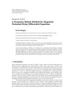
Figure 2: Solutions of nonlinear stiff system for α 1, a Exact, b Numerical, c NHPM, and c NHPM,
α 0.9, 1/3 color figure can be viewed in the online issue.
00.51
w
u
v
1.522.5
−0.3
−0.2
−0.1
0
0.1
0.2
0.3
t
0.4
u, v
a
00.511.522.5
−0.3
−0.2
−0.1
w
u
v
0
0.1
0.2
0.3
t
0.4
u, v
b
00.511.52
α
1
2
w
u
v
−0.3
−0.2
−0.1
0
0.1
0.2
0.3
t
0.4
u, v
c
00.511.52
−0.3
α 0.75 w
u
v
−0.2
−0.1
0
0.1
0.2
0.3
t
0.4
u, v
d
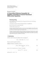
Figure 3: Solutions of nonlinear Genesio system for a Numerical, b NHPM α 1, c NHPM, α 0.5,
d NHPM, α 0.75 color figure can be viewed in the online issue.
14 Advances in Difference Equations
00.511.52 32.5
−4
−6
−2
0
2
6
4
t
u, v
a
00.511.52 32.5
−2
−4
0
2
4
t
u, v
b
00.511.52 32.5
−5
−10
0
5
10
t
u, v
c
Figure 4: Solutions of matrix Riccati equations u w, v z for α 1 a Numerical, b NHPM-Pade
9/11, c NHPM-Pade 9/11, α 0.5 color figure can be viewed in the online issue.
Acknowledgment
M. Jamil is highly thankful and grateful to the Abdus Salam School of Mathematical Sciences,
GC University, Lahore, Pakistan, the Department of Mathematics & Basic Sciences, NED
University of Engineering & Technology, Karachi-75270, Pakistan, and also the Higher
Education Commission of Pakistan for generously supporting and facilitating this research
work.
References
1 H. M. Kilbas, H. M. Srivastava, and J. J. Trujillo, Theory and A pplications of Fractional Differential
Equations, Elsevier, Amsterdam, The Netherlands, 2007.
2 R. L. Bagley and R. A. Calico, “Fractional order state equations for the control of viscoelastically
damped structures,” Journal of Guidance, Control, and Dynamics, vol. 14, no. 2, pp. 304–311, 1991.
3 A.Mahmood,S.Parveen,A.Ara,andN.A.Khan,“Exactanalyticsolutionsfortheunsteadyflowof
a non-Newtonian fluid between two cylinders with fractional derivative model,” Communications in
Nonlinear Science and Numerical Simulation, vol. 14, no. 8, pp. 3309–3319, 2009.
4 A. Mahmood, C. Fetecau, N. A. Khan, and M. Jamil, “Some exact solutions of the oscillatory motion
of a generalized second grade fluid in an annular region of two cylinders,” Acta Mechanica Sinica,vol.
26, no. 4, pp. 541–550, 2010.
5 J. H. He, “Nonlinear oscillation with fractional derivative and its applications,” in Proceedings of the
International Conference on Vibrating Engineering, pp. 288–291, Dalian, China, 1998.
Advances in Difference Equations 15
6 N. A. Khan, N U. Khan, A. Ara, and M. Jamil, “Approximate analytical solutionsof fractional
reaction-diffusion equations,” Journal of King Saud University—Science. In press.
7 J H. He, “Homotopy perturbation technique,” Computer Methods in Applied Mechanics and Engineering,
vol. 178, no. 3-4, pp. 257–262, 1999.
8 J H. He, “A coupling method of a homotopy technique and a perturbation technique for non-linear
problems,” International Journal of Non-Linear Mechanics, vol. 35, no. 1, pp. 37–43, 2000.
9 J H. He, “Homotopy perturbation method: a new nonlinear analytical technique,” Applied
Mathematics and Computation, vol. 135, no. 1, pp. 73–79, 2003.
10 N. A. Khan, A. Ara, and A. Mahmood, “Approximate solution of time-fractional chemical engineering
equations: a comparative study,” International Journal of Chemical Reactor Engineering,vol.8,article
A19, 2010.
11 N. A. Khan, N U. Khan, M. Ayaz, and A. Mahmood, “Analytical methods for solving the time-
fractional Swift-Hohenberg S-H equation,” Computers and Mathematics with Applications. In press.
12 N. A. Khan, A. Ara, S. A. Ali, and M. Jamil, “Orthognal flow impinging on a wall with suction or
blowing,” International Journal of Chemical Reactor Engineering. In press.
13 A. Yıldırım, “Solution of BVPs for fourth-order integro-differential equations by using homotopy
perturbation method,” Computers & Mathematics with Applications, vol. 56, no. 12, pp. 3175–3180, 2008.
14 H. Koc¸ak, T.
¨
Ozis¸, and A. Yıldırım, “Homotopy perturbation method for the nonlinear dispersive
Km,n,1 equations with fractional time derivatives,” International Journal of Numerical Methods for
Heat & Fluid Flow, vol. 20, no. 2, pp. 174–185, 2010.
15 Y. Khan, N. Faraz, A. Yildirim, and Q. Wu, “A series solution of the long porous slider,” Tr ibology
Transac t i o n s , vol. 54, no. 2, pp. 187–191, 2011.
16 N. A. Khan, A. Ara, S. A. Ali, and A. Mahmood, “Analytical study of Navier-Stokes equation with
fractional orders using He’s homotopy perturbation and variational iteration methods,” International
Journal of Nonlinear Sciences and Numerical Simulation, vol. 10, no. 9, pp. 1127–1134, 2009.
17 H. Aminikhah and J. Biazar, “A new HPM for ordinary differential equations,” Numerical Methods for
Partial Differential Equations, vol. 26, no. 2, pp. 480–489, 2010.
18 H. Aminikhah and M. Hemmatnezhad, “An efficient method for quadratic Riccati differential
equation,” Communications in Nonlinear Science and Numerical Simulation, vol. 15, no. 4, pp. 835–839,
2010.
19 Y. Khan and N. Faraz, “Modified fractional decomposition method having integral w.r.t dξ
α
,”
Journal of King Saud University—Science. In press.
20 A. S. Bataineh, M. S. M. Noorani, and I. Hashim, “Solving systems of ODEs by homotopy analysis
method,” Communications in Nonlinear Science and Numerical Simulation, vol. 13, no. 10, pp. 2060–2070,
2008.