Sustainable Wireless Sensor Networks Part 12 ppt

Sustainable Wireless Sensor Networks376

complete round. It is calculated for each sensor according to its distance from the sink. A
sensor that has energy below this threshold, cannot act as an NM for the network. Sensors
are classified according to these thresholds before NM selection into one of three categories:
1) Active nodes that can act as NMs. 2) Active nodes but cannot act as NMs and 3) Inactive
nodes or dead nodes.
Once a node is classified as a dead node, the network is considered dead, according to the
definition of lifetime used in this study. The sink has knowledge about the whole network
and is responsible for selecting the NM and informs all other sensors about the current NM.
It selects a sensor as an NM for the current round according to the following criteria. 1) The
node belongs to the first category. 2) The node has energy greater than the average energy of
all active nodes and 3) The sum of its distances to the active nodes is least. In this algorithm,
it is assumed that a node can be selected as an NM for many rounds throughout network
lifetime. A simulation model is built using MATLAB (MatLab) with the same network
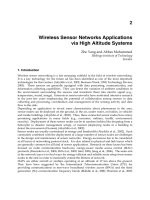
parameters used in (Heinzelman et al., 2002) and described above. The system is run for
different values of the number of cycles “C” per round, and the corresponding network
lifetime is as shown in Fig. 1. The figure shows that there is an optimum number of cycles
for which each sensor remains acting as NM, before another round starts over and a new
NM is selected. For the parameters considered, the longest lifetime is achieved for “C=3”,
resulting in a lifetime equivalent to “3702” cycles.

0 2 4 6 8 10 12 14
3350
3400
3450
3500
3550
3600
3650
3700

3750
X: 3
Y: 3702
Optimizing the number of Cycles per Round
Number of Cycles per Round
Total Lifetime in Cycles

Fig. 1. Network lifetime vs number of cycles per round

2.4 Algorithm II
The previous algorithm selected a fixed optimum number of cycles “C” per round in order
to achieve a longer lifetime. It is observed that with this relatively small number of cycles, a
sensor is chosen as an NM for many rounds. It is observed also that not all sensors act as
NMs for the same number of rounds. So, if these could be gathered together such that each
sensor is selected as an NM only once, but without exhausting sensors which require more
energy to act as an NM, a longer lifetime for the network will be achieved. Another
observation in previous techniques is that after the death of the first node, there is still some
residual energy for some sensors. This residual energy is not used efficiently. One reason is
that it is distributed to all the sensors, and hence, the share of each sensor is not large

enough to work as NM. Another reason is that the full coverage of the network, which may
be a primary concern in many applications, is lost. Both observations lead to an algorithm
which requires that each sensor be selected as an NM only once, and acts as an NM for a
certain number of cycles “C
i
”, which need not be the same for all sensors. The algorithm also
requires the most usage of the available energies for each sensor.
The algorithm is simply run once at the sink based on its knowledge of the locations of the
different sensors. The sink can calculate the energy “E
txi to NM j

” required by each sensor “i” to
transmit its data to any of the other nodes “j” acting as an NM, as well as the energy “E
NMi
”
needed by the node “i" to act as an NM itself. Assuming that each sensor acts as an NM for a
certain number of cycles “C
i
”, before and after which it acts as an ordinary node, the energy
consumed by any sensor “i” through the network lifetime can be calculated as:






Nj
ij
j
NMjtxijNMiiisensor
ECECE
1
to

(1)
for
Ni ,,2,1 
Since each sensor will act as a NM only once for “C
i
” cycles, then the total lifetime, in
number of cycles, is the summation of the different “C

i
”s.



i
i
CT
(2)

If each sensor node “i” has an initial energy “E
o i
”, it must be that the energy consumed by
any sensor is less than or equal its initial energy. That is:

iisensor
EE
0


(3)

In order to make the best use of the available energies for the sensor, the following set of
“N” equations in “N” unknowns, { C
1
, C
2
, C
3
, … , C

N
}, is solved.

iisensor
EE
0


(4)
for
Ni ,,2,1 

10 20 30 40 50 60 70 80 90 100
0
5
10
15
20
25
30
35
40
45
50
Sensors
Number of Cycles

Fig. 2. Number of cycles “C
i
” assigned to each sensor to act as a Network Master

Node Deployment and Mobile Sinks for Wireless Sensor Networks Lifetime Improvement 377

complete round. It is calculated for each sensor according to its distance from the sink. A
sensor that has energy below this threshold, cannot act as an NM for the network. Sensors
are classified according to these thresholds before NM selection into one of three categories:
1) Active nodes that can act as NMs. 2) Active nodes but cannot act as NMs and 3) Inactive
nodes or dead nodes.
Once a node is classified as a dead node, the network is considered dead, according to the
definition of lifetime used in this study. The sink has knowledge about the whole network
and is responsible for selecting the NM and informs all other sensors about the current NM.
It selects a sensor as an NM for the current round according to the following criteria. 1) The
node belongs to the first category. 2) The node has energy greater than the average energy of
all active nodes and 3) The sum of its distances to the active nodes is least. In this algorithm,
it is assumed that a node can be selected as an NM for many rounds throughout network
lifetime. A simulation model is built using MATLAB (MatLab) with the same network
parameters used in (Heinzelman et al., 2002) and described above. The system is run for
different values of the number of cycles “C” per round, and the corresponding network
lifetime is as shown in Fig. 1. The figure shows that there is an optimum number of cycles
for which each sensor remains acting as NM, before another round starts over and a new
NM is selected. For the parameters considered, the longest lifetime is achieved for “C=3”,
resulting in a lifetime equivalent to “3702” cycles.

0 2 4 6 8 10 12 14
3350
3400
3450
3500
3550
3600
3650

3700
3750
X: 3
Y: 3702
Optimizing the number of Cycles per Round
Number of Cycles per Round
Total Lifetime in Cycles

Fig. 1. Network lifetime vs number of cycles per round

2.4 Algorithm II
The previous algorithm selected a fixed optimum number of cycles “C” per round in order
to achieve a longer lifetime. It is observed that with this relatively small number of cycles, a
sensor is chosen as an NM for many rounds. It is observed also that not all sensors act as
NMs for the same number of rounds. So, if these could be gathered together such that each
sensor is selected as an NM only once, but without exhausting sensors which require more
energy to act as an NM, a longer lifetime for the network will be achieved. Another
observation in previous techniques is that after the death of the first node, there is still some
residual energy for some sensors. This residual energy is not used efficiently. One reason is
that it is distributed to all the sensors, and hence, the share of each sensor is not large

enough to work as NM. Another reason is that the full coverage of the network, which may
be a primary concern in many applications, is lost. Both observations lead to an algorithm
which requires that each sensor be selected as an NM only once, and acts as an NM for a
certain number of cycles “C
i
”, which need not be the same for all sensors. The algorithm also
requires the most usage of the available energies for each sensor.
The algorithm is simply run once at the sink based on its knowledge of the locations of the
different sensors. The sink can calculate the energy “E

txi to NM j
” required by each sensor “i” to
transmit its data to any of the other nodes “j” acting as an NM, as well as the energy “E
NMi
”
needed by the node “i" to act as an NM itself. Assuming that each sensor acts as an NM for a
certain number of cycles “C
i
”, before and after which it acts as an ordinary node, the energy
consumed by any sensor “i” through the network lifetime can be calculated as:






Nj
ij
j
NMjtxijNMiiisensor
ECECE
1
to

(1)
for
Ni ,,2,1 
Since each sensor will act as a NM only once for “C
i
” cycles, then the total lifetime, in

number of cycles, is the summation of the different “C
i
”s.



i
i
CT
(2)

If each sensor node “i” has an initial energy “E
o i
”, it must be that the energy consumed by
any sensor is less than or equal its initial energy. That is:

iisensor
EE
0

(3)

In order to make the best use of the available energies for the sensor, the following set of
“N” equations in “N” unknowns, { C
1
, C
2
, C
3
, … , C

N
}, is solved.

iisensor
EE
0


(4)
for
Ni ,,2,1 

10 20 30 40 50 60 70 80 90 100
0
5
10
15
20
25
30
35
40
45
50
Sensors
Number of Cycles

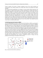
Fig. 2. Number of cycles “C
i
” assigned to each sensor to act as a Network Master

Sustainable Wireless Sensor Networks378

The solution set S = {C
i
} indicates that the network will have maximum lifetime. Any other
set, S’ = {C
i
’}, will not be a solution for the set of equations. It should be noted that the
solution of such equations does not guarantee integer values for the “C
i
”s; therefore, the
fractional part of the solution set must be truncated. The simulation environment used
before is used for the new scheme. The solution of the set of equations in (4) resulted in the
set of “C
i
”s shown in Fig. 2 after truncation. It can be observed that the different values of
“C
i
” range between 16 and 46 cycles per round. The summation of these “C
i
”s causes the
expected lifetime of the network to be almost 3900 cycles which is higher than the lifetime
obtained from the first algorithm.

2.5 Geometric distributions
Random distributions, which were used in (Botros et al., 2009), are more suitable for certain
applications where the network locations are inaccessible (Tavares et al., 2008), such as
military applications. However, as mentioned before, in some applications (such as urban
applications), the deployment of nodes at pre-specified positions is feasible (Onur et al.,
2007). Hence, this subsection focuses on geometric distributions instead of random

distribution and their effect on maximizing the network's lifetime.

2.5.1 Star topology
The Star topology is one of the most common geometric distributions used in networks
(Cheng & Liu, 2004; Bose & Helal, 2008). Therefore star topologies are chosen for testing as
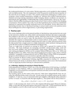
geometric distributions. By using the same previous parameters (Botros et al., 2009), it is
found that the star with 3 branches and 33 sensors per branch (3×33 star) produces 5%
increase in network lifetime. Furthermore, several stars with different numbers of branches
are generated for simulation. The main characteristics for the used star distributions in this
study are as follows:
 Sensors are distributed in circles from the centre to the borders of the area and each
circle has an equal number of sensors.
 Equal angles between branches and equal distances between sensors in the same
branch.

-50 -40 -30 -20 -10 0 10 20 30 40 50
-50
-40
-30
-20
-10
0
10
20
30
40
50

Fig. 3. 3x33 Star

The number of branches that were tested ranges between 3 and 20 with a suitable number of
sensors in each circle to constitute the used number of sensors which is N=100 sensors used
by (Botros et al., 2009; Minet & Mahfoudh, 2009). The 3×33 star (shown in Fig. 3) has 3
branches, 33 sensors per branch and the 100
th
sensor is located in the center of the star. The
network parameters used in this study are as follows:
 Number of Sensors (N): 100 Sensors
 Initial Energy: 2 J
 Transmitter/ Receiver Electronics: 50 nJ/bit
 Transmitter Amplifier : 100 pJ/bit/m
2

 Path Loss factor: 2
 Aggregation Energy: 5 nJ/bit/Signal
 Data packet size (K): 2000 bits
 Sink location: (0; 125)

2.5.2Proposed algorithm
A simulation model is built using MATLAB considering the above network parameters. The
lifetime in case of geometric distributions is computed by using the algorithm described in
section 2.4.

2.5.3 Simulations and results
By simulating the proposed algorithm with different star distributions, it was found that the
333 star achieves the maximum lifetime compared to the other star distributions as shown
in Table 2. It was found that the 333 star extends the lifetime of the network by 35.6%
compared to the random distribution used in (Botros et al., 2009). The numbers of sensors
that can act as NMs in 333 star were 70 out of 100 sensors and the number of cycles
allocated for each NM are as shown in Fig. 4. All the simulations results are specific to the

orientation of the used topology.

Star Distribution Lifetime (Cycles)
3x33 4612
4x25 4510
5x20 4278
6x16 4346
7x14 4437
8x12 4399
9x11 4510
10x10 4466
12x8 4314
14x7 4388
20x5 4412
Table 2. Lifetimes of different star distributions

Node Deployment and Mobile Sinks for Wireless Sensor Networks Lifetime Improvement 379

The solution set S = {C
i
} indicates that the network will have maximum lifetime. Any other
set, S’ = {C
i
’}, will not be a solution for the set of equations. It should be noted that the
solution of such equations does not guarantee integer values for the “C
i
”s; therefore, the
fractional part of the solution set must be truncated. The simulation environment used
before is used for the new scheme. The solution of the set of equations in (4) resulted in the
set of “C

i
”s shown in Fig. 2 after truncation. It can be observed that the different values of
“C
i
” range between 16 and 46 cycles per round. The summation of these “C
i
”s causes the
expected lifetime of the network to be almost 3900 cycles which is higher than the lifetime
obtained from the first algorithm.

2.5 Geometric distributions
Random distributions, which were used in (Botros et al., 2009), are more suitable for certain
applications where the network locations are inaccessible (Tavares et al., 2008), such as
military applications. However, as mentioned before, in some applications (such as urban
applications), the deployment of nodes at pre-specified positions is feasible (Onur et al.,
2007). Hence, this subsection focuses on geometric distributions instead of random
distribution and their effect on maximizing the network's lifetime.

2.5.1 Star topology
The Star topology is one of the most common geometric distributions used in networks
(Cheng & Liu, 2004; Bose & Helal, 2008). Therefore star topologies are chosen for testing as
geometric distributions. By using the same previous parameters (Botros et al., 2009), it is
found that the star with 3 branches and 33 sensors per branch (3×33 star) produces 5%
increase in network lifetime. Furthermore, several stars with different numbers of branches
are generated for simulation. The main characteristics for the used star distributions in this
study are as follows:
 Sensors are distributed in circles from the centre to the borders of the area and each
circle has an equal number of sensors.
 Equal angles between branches and equal distances between sensors in the same
branch.

-50 -40 -30 -20 -10 0 10 20 30 40 50
-50
-40
-30
-20
-10
0
10
20
30
40
50

Fig. 3. 3x33 Star

The number of branches that were tested ranges between 3 and 20 with a suitable number of
sensors in each circle to constitute the used number of sensors which is N=100 sensors used
by (Botros et al., 2009; Minet & Mahfoudh, 2009). The 3×33 star (shown in Fig. 3) has 3
branches, 33 sensors per branch and the 100
th
sensor is located in the center of the star. The
network parameters used in this study are as follows:
 Number of Sensors (N): 100 Sensors
 Initial Energy: 2 J
 Transmitter/ Receiver Electronics: 50 nJ/bit
 Transmitter Amplifier : 100 pJ/bit/m
2

 Path Loss factor: 2

 Aggregation Energy: 5 nJ/bit/Signal
 Data packet size (K): 2000 bits
 Sink location: (0; 125)

2.5.2Proposed algorithm
A simulation model is built using MATLAB considering the above network parameters. The
lifetime in case of geometric distributions is computed by using the algorithm described in
section 2.4.

2.5.3 Simulations and results
By simulating the proposed algorithm with different star distributions, it was found that the
333 star achieves the maximum lifetime compared to the other star distributions as shown
in Table 2. It was found that the 333 star extends the lifetime of the network by 35.6%
compared to the random distribution used in (Botros et al., 2009). The numbers of sensors
that can act as NMs in 333 star were 70 out of 100 sensors and the number of cycles
allocated for each NM are as shown in Fig. 4. All the simulations results are specific to the
orientation of the used topology.

Star Distribution Lifetime (Cycles)
3x33 4612
4x25 4510
5x20 4278
6x16 4346
7x14 4437
8x12 4399
9x11 4510
10x10 4466
12x8 4314
14x7 4388
20x5 4412

Table 2. Lifetimes of different star distributions

Sustainable Wireless Sensor Networks380

0 10 20 30 40 50 60 70 80 90 100
0
10
20
30
40
50
60
70
80
90
100

Fig. 4. Number of cycles for each NM in a 3x33star

2.6 Sink locations
The different star distributions used in the previous section were tested to achieve the best
distribution with respect to the lifetime using the sink location at (0; 125) which was used
by (Botros et al., 2009). The results showed that 333 star produces the highest lifetime. This
result was taken a step further by applying other sink locations in order to explore the effect
of the other sink locations on network lifetime. The sink locations used in this study are (0;
125), (125; 0), (125; 0), (125; 125), (125; 125), (125; 125), (125; 125) and (0; 0).
Simulating the different sink locations on the best star (333 star) results in better and worse
lifetime with respect to the (0; 125) sink location. But the objective is to increase network
lifetime, so sink locations that achieve higher lifetime are of great concern. The (0; 0) sink
location increased the network’s lifetime of the 333 star from 4612 cycles, in the case of the

(0; 125), to 5205 cycles, which is an improvement of approximately 13%.
In order to find the reason why changing the sink location to (0; 0) increases the lifetime,
some calculations were computed to measure the total distance traveled by data. As
mentioned before, each sensor acted as a NM for a certain number of cycles for only one
round. This NM collects data from all other sensors, aggregates it then sends the aggregated
data to the sink. Therefore, two communication distances must be measured for each sensor
as follows:


NMsensor
d

;

which is the communication distance between every sensor and the selected NM.


SinkNM
d



which is the communication distance between the selected NM and the sink. By adding all
the distances between the sensors and every NM and the distance between every NM and
the sink, a new metric is derived as follows:


 




 




M
j
M
j
SinkNM
N
ji
i
NMsensordata
j
ji
ddd
1 11

(5)
where N is the number of sensors and M is the number of NMs. Comparing the distance
travelled by data for each sink location, it was found that at sink (0;0),
data
d was the lowest.

2.7 Uniform distributions
Using the star topologies was successful in prolonging the lifetime of the network. But the
star distributions are not suitable for all WSN applications. Some WSN applications such as
chemical, environmental and nuclear sensing systems require uniformly distributed sensors

(Bestavros et al., 2004). Therefore, some distributions with uniform densities were
investigated in this study. The distributions were tested at the different sink locations and it
was found that the maximum lifetime was obtained at the (0; 0) sink location. First, the
hexagonal distribution was tested due to its wide and comprehensive coverage (Prabh et al.,
2009; Gui & He, 2009). The second distribution is the Homogeneous Density Distribution in
which a sensor was placed every meter square over the entire area (see Fig. 5). Finally, a
circular distribution is tested with uniform density in which the number of sensors per circle
increased as they move towards the border of the area. The homogeneous density
distribution resulted the highest lifetime compared to the other uniform distributions. It
produced 3301 cycle, while the hexagonal and the circular distributions produced only 3293
and 2876 cycles respectively.

-50 -40 -30 -20 -10 0 10 20 30 40 50
-50
-40
-30
-20
-10
0
10
20
30
40
50

Fig. 5. Homogeneous Density Distribution

3. Relaying data collection
The fact that a sensor drains much of its power in trying to send its data to a fixed sink
makes it necessary to use a mobile sink in addition to the fixed one. This is called a hybrid

system. This section considers the problem of maximizing system life time (i.e., reducing
the energy consumption) by properly choosing the destination; either the fixed sink or
the mobile one (which is not controlled). More details about this work can be found in
Node Deployment and Mobile Sinks for Wireless Sensor Networks Lifetime Improvement 381

0 10 20 30 40 50 60 70 80 90 100
0
10
20
30
40
50
60
70
80
90
100

Fig. 4. Number of cycles for each NM in a 3x33star

2.6 Sink locations
The different star distributions used in the previous section were tested to achieve the best
distribution with respect to the lifetime using the sink location at (0; 125) which was used
by (Botros et al., 2009). The results showed that 333 star produces the highest lifetime. This
result was taken a step further by applying other sink locations in order to explore the effect
of the other sink locations on network lifetime. The sink locations used in this study are (0;
125), (125; 0), (125; 0), (125; 125), (125; 125), (125; 125), (125; 125) and (0; 0).
Simulating the different sink locations on the best star (333 star) results in better and worse
lifetime with respect to the (0; 125) sink location. But the objective is to increase network
lifetime, so sink locations that achieve higher lifetime are of great concern. The (0; 0) sink

location increased the network’s lifetime of the 333 star from 4612 cycles, in the case of the
(0; 125), to 5205 cycles, which is an improvement of approximately 13%.
In order to find the reason why changing the sink location to (0; 0) increases the lifetime,
some calculations were computed to measure the total distance traveled by data. As
mentioned before, each sensor acted as a NM for a certain number of cycles for only one
round. This NM collects data from all other sensors, aggregates it then sends the aggregated
data to the sink. Therefore, two communication distances must be measured for each sensor
as follows:


NMsensor
d

;

which is the communication distance between every sensor and the selected NM.


SinkNM
d



which is the communication distance between the selected NM and the sink. By adding all
the distances between the sensors and every NM and the distance between every NM and
the sink, a new metric is derived as follows:


 




 




M
j
M
j
SinkNM
N
ji
i
NMsensordata
j
ji
ddd
1 11

(5)
where N is the number of sensors and M is the number of NMs. Comparing the distance
travelled by data for each sink location, it was found that at sink (0;0),
data
d was the lowest.

2.7 Uniform distributions
Using the star topologies was successful in prolonging the lifetime of the network. But the
star distributions are not suitable for all WSN applications. Some WSN applications such as

chemical, environmental and nuclear sensing systems require uniformly distributed sensors
(Bestavros et al., 2004). Therefore, some distributions with uniform densities were
investigated in this study. The distributions were tested at the different sink locations and it
was found that the maximum lifetime was obtained at the (0; 0) sink location. First, the
hexagonal distribution was tested due to its wide and comprehensive coverage (Prabh et al.,
2009; Gui & He, 2009). The second distribution is the Homogeneous Density Distribution in
which a sensor was placed every meter square over the entire area (see Fig. 5). Finally, a
circular distribution is tested with uniform density in which the number of sensors per circle
increased as they move towards the border of the area. The homogeneous density
distribution resulted the highest lifetime compared to the other uniform distributions. It
produced 3301 cycle, while the hexagonal and the circular distributions produced only 3293
and 2876 cycles respectively.

-50 -40 -30 -20 -10 0 10 20 30 40 50
-50
-40
-30
-20
-10
0
10
20
30
40
50

Fig. 5. Homogeneous Density Distribution

3. Relaying data collection
The fact that a sensor drains much of its power in trying to send its data to a fixed sink

makes it necessary to use a mobile sink in addition to the fixed one. This is called a hybrid
system. This section considers the problem of maximizing system life time (i.e., reducing
the energy consumption) by properly choosing the destination; either the fixed sink or
the mobile one (which is not controlled). More details about this work can be found in
Sustainable Wireless Sensor Networks382

(Zaki et al., 2008; Zaki et al. 2009). Using a hybrid model for message relaying, an energy
balancing scheme is proposed in a linear low mobility wireless sensor network. The system
uses either a single hop transmission to a nearby mobile sink or a multi-hop transmission to
a far-away fixed sink depending on the predicted sink mobility pattern. Taking a
mathematical approach, the system parameters are adjusted so that all the sensor nodes
dissipate the same amount of energy. Simulation results showed that the proposed system
outperforms classical methods of message gathering in terms of system lifetime. On the
single node level, the average total energy consumed by the hybrid system is equalized over
all sensors and the problem of losing connectivity due to the fast power drainage of the
closest node to the fixed sink, is resolved.

3.1 System description
Fixed wireless sensor networks are described in the form of two tiers: the sensor and the
fixed sink (observer). Another approach is the introduction of a third tier which is the
mobile sink. Sensors send their data to the mobile sink as the second relay point instead of
sending to the fixed sink. There are many benefits of using this approach where the most
important is the reduction of power consumption during the transmission phase. The sensor
is not required anymore to send its messages to faraway points as the mobile sink
approaches the sensor to get the data. This system has many other advantages including
robustness against the failure of nodes, higher network connectivity and reduction of the
control messages overhead required to set up paths to the observer (Al-Karaki & Kamal,
2004).
The Data Mules (Shah et al., 2003), approach aims at addressing the operation of using
existing mobile sinks, termed MULEs (Mobile Ubiquitous LAN Extensions) to collect sensed

data in the environment. In a vehicular traffic monitoring application, the vehicles can serve
as mobile agents, whereas in a wildlife tracking application, the animals can be used as
mobile agents. The MULEs are fitted with transceivers that are capable of short-range
wireless communication. They can exchange data with sensors and access points when they
move into their vicinity. The main disadvantage of the basic implementation of the Data
Mules scheme is its high latency. Each sensor node needs to wait for a MULE to come within
its transmission radius before it can transfer its readings. Another disadvantage is that the
system assumes the existence of mobile agents in the target environment, which may not
always be true. The sensor nodes need to keep their radio receivers on continuously to be
able to communicate with MULEs. In this section, a hybrid message transmission system
that takes advantages of the data MULEs concept as well as the basic protocols of data
routing, is developed. The system solves the inherit disadvantages of the basic MULEs
architecture and increases network lifetime by reducing the single node power consumption
and by balancing the overall system energy.
A typical three layers architecture for environmental monitoring system in urban areas
consists of (Jain et al., 2006):
 The lowest layer consists of different types of sensor nodes.
 The second layer consists of the mobile agent that can be a moving car, a personal
digital assistant or any moving device.
 The higher layer consists of the fixed sink. It represents the collection point of the
sensed data before its transmission through a WAN to a monitoring point.


Considering this architecture for a city, a large number of fixed sensor nodes are deployed
on both sides of the street to monitor different phenomena. Sensors work on their limited
energy reservoir. Fixed sinks are the collection points that receive the sensed data directly
from the sensor modules or from mobile sinks. They have higher capability than the sensor
modules in terms of computational power and connectivity. The number of fixed sinks is
usually smaller than the number of sensors; that is why it is not a costly operation to connect
them to permanent power supplies or large energy scavenger and different communications

facilities. When the sensed data is received by the fixed sinks, it can be forwarded to central
databases through the wired or wireless infrastructure network for further processing. The
mobile sinks periodically broadcast a beacon to notify nearby sensors of their existence.
Upon reception of the beacon message, the sensor module can transmit its data to the
nearby mobile node as the next overlay, thus saving its energy. The mobile agent can then
send the sensed data to the fixed sink or to the remote database using other communication
means.

3.2 Underlying system models
The models used in the system under study are explained next.

3.2.1 Routing, MAC and mobility models
The fixed part of the network operates the routing protocol suggested in (Younis et al.,
2002). The basic assumptions are:
1. Appling a MAC protocol that allows the sensor to listen to the channel in a specified
time slot as TDMA based protocol that minimizes the idle listening power when
routing to fixed points.
2. The gateway which can be seen as the fixed sink has high computational power. All
system algorithms are run on the gateway and the system parameter values are then
broadcasted to the sensor nodes.
3. The sensor can determine transmission distance to its next hop and adjust its power
amplifier correspondingly.
4. The radio transceiver can be turned on and off.

In mobile sink WSN, various basic approaches for mobility are involved: random, controlled
and predictable. Random objects such as humans and animals can be used to relay the
sensed data when they are in the coverage range. As the main issue in the described system
is the moving cars in a street, therefore only one-dimensional uncontrolled mobility is
considered. Different techniques are used to model vehicular traffic flows (Hoogendorn &
Bovy, 2001). One well known example of mesoscopic model is the headway distribution

model where it expresses the vehicular time headway as a probability distribution (Al-
Ghamdi, 2001). Typical distributions are negative exponential and gamma distributions. The
inter-arrival time T between two successive cars is modeled as a negative exponential
distribution with an average β.

 



T
eTF


1
,

(6)
Node Deployment and Mobile Sinks for Wireless Sensor Networks Lifetime Improvement 383

(Zaki et al., 2008; Zaki et al. 2009). Using a hybrid model for message relaying, an energy
balancing scheme is proposed in a linear low mobility wireless sensor network. The system
uses either a single hop transmission to a nearby mobile sink or a multi-hop transmission to
a far-away fixed sink depending on the predicted sink mobility pattern. Taking a
mathematical approach, the system parameters are adjusted so that all the sensor nodes
dissipate the same amount of energy. Simulation results showed that the proposed system
outperforms classical methods of message gathering in terms of system lifetime. On the
single node level, the average total energy consumed by the hybrid system is equalized over
all sensors and the problem of losing connectivity due to the fast power drainage of the
closest node to the fixed sink, is resolved.

3.1 System description
Fixed wireless sensor networks are described in the form of two tiers: the sensor and the
fixed sink (observer). Another approach is the introduction of a third tier which is the
mobile sink. Sensors send their data to the mobile sink as the second relay point instead of
sending to the fixed sink. There are many benefits of using this approach where the most
important is the reduction of power consumption during the transmission phase. The sensor
is not required anymore to send its messages to faraway points as the mobile sink
approaches the sensor to get the data. This system has many other advantages including
robustness against the failure of nodes, higher network connectivity and reduction of the
control messages overhead required to set up paths to the observer (Al-Karaki & Kamal,
2004).
The Data Mules (Shah et al., 2003), approach aims at addressing the operation of using
existing mobile sinks, termed MULEs (Mobile Ubiquitous LAN Extensions) to collect sensed
data in the environment. In a vehicular traffic monitoring application, the vehicles can serve
as mobile agents, whereas in a wildlife tracking application, the animals can be used as
mobile agents. The MULEs are fitted with transceivers that are capable of short-range
wireless communication. They can exchange data with sensors and access points when they
move into their vicinity. The main disadvantage of the basic implementation of the Data
Mules scheme is its high latency. Each sensor node needs to wait for a MULE to come within
its transmission radius before it can transfer its readings. Another disadvantage is that the
system assumes the existence of mobile agents in the target environment, which may not
always be true. The sensor nodes need to keep their radio receivers on continuously to be
able to communicate with MULEs. In this section, a hybrid message transmission system
that takes advantages of the data MULEs concept as well as the basic protocols of data
routing, is developed. The system solves the inherit disadvantages of the basic MULEs
architecture and increases network lifetime by reducing the single node power consumption
and by balancing the overall system energy.
A typical three layers architecture for environmental monitoring system in urban areas
consists of (Jain et al., 2006):
 The lowest layer consists of different types of sensor nodes.

 The second layer consists of the mobile agent that can be a moving car, a personal
digital assistant or any moving device.
 The higher layer consists of the fixed sink. It represents the collection point of the
sensed data before its transmission through a WAN to a monitoring point.


Considering this architecture for a city, a large number of fixed sensor nodes are deployed
on both sides of the street to monitor different phenomena. Sensors work on their limited
energy reservoir. Fixed sinks are the collection points that receive the sensed data directly
from the sensor modules or from mobile sinks. They have higher capability than the sensor
modules in terms of computational power and connectivity. The number of fixed sinks is
usually smaller than the number of sensors; that is why it is not a costly operation to connect
them to permanent power supplies or large energy scavenger and different communications
facilities. When the sensed data is received by the fixed sinks, it can be forwarded to central
databases through the wired or wireless infrastructure network for further processing. The
mobile sinks periodically broadcast a beacon to notify nearby sensors of their existence.
Upon reception of the beacon message, the sensor module can transmit its data to the
nearby mobile node as the next overlay, thus saving its energy. The mobile agent can then
send the sensed data to the fixed sink or to the remote database using other communication
means.

3.2 Underlying system models
The models used in the system under study are explained next.

3.2.1 Routing, MAC and mobility models
The fixed part of the network operates the routing protocol suggested in (Younis et al.,
2002). The basic assumptions are:
1. Appling a MAC protocol that allows the sensor to listen to the channel in a specified
time slot as TDMA based protocol that minimizes the idle listening power when
routing to fixed points.

2. The gateway which can be seen as the fixed sink has high computational power. All
system algorithms are run on the gateway and the system parameter values are then
broadcasted to the sensor nodes.
3. The sensor can determine transmission distance to its next hop and adjust its power
amplifier correspondingly.
4. The radio transceiver can be turned on and off.

In mobile sink WSN, various basic approaches for mobility are involved: random, controlled
and predictable. Random objects such as humans and animals can be used to relay the
sensed data when they are in the coverage range. As the main issue in the described system
is the moving cars in a street, therefore only one-dimensional uncontrolled mobility is
considered. Different techniques are used to model vehicular traffic flows (Hoogendorn &
Bovy, 2001). One well known example of mesoscopic model is the headway distribution
model where it expresses the vehicular time headway as a probability distribution (Al-
Ghamdi, 2001). Typical distributions are negative exponential and gamma distributions. The
inter-arrival time T between two successive cars is modeled as a negative exponential
distribution with an average β.

 



T
eTF


1
,

(6)

Sustainable Wireless Sensor Networks384

During a 24-hour period, the traffic flow rate varies between heavy traffic during rush hours
and low traffic at the end of day. Therefore, the one day cycle can be divided into several
time intervals in which the value of β is considered constant.

3.2.2 Energy model
There are three basic operations in which sensors consume their energy (Shebli et al., 2007).
First the sensor node has to convert the sensed phenomena to a digital signal. This is called
aquisition. Second, the digital signal may be processed before transmission. Finally the
sensor has to wirelessly communicate the data it aquire or receives. In this work, the focus is
on the communication operation which is the basic source of power consumption.
The wireless node transceiver may be in one of four states:
1. sending a message,
2. receiving a message,
3. idle listening for a message,
4. in the low power sleep mode.

The linear transceiver model is used where:
1. The energy consumed to send a frame of size m over a distance of d meters consists of
two main parts: the first one represents the energy dissipated in the transmitter and the
second represents the energy dissipated in the power amplifier.





k
ampelecTX
deemdmE ,

(7)

where m is the message length in bits, e
elec
is the amount of energy consumed by the
transmitter circuits to modulate one bit and e
anp
d
K
is the amount of energy dissipated in
the power amplifier in order to reach acceptable signal to noise ratio at the receiver that
is located d meters away. k is an integer constant that varies between two to four
depending on the surrounding medium. e
anp
takes into account the antenna gain at the
transmitter and the receiver:
2. To receive an m bits long message, the receiver then consumes:



rxRX
emmE 
(8)

where e
rx
represents the reception energy per bit and m the message length. In order to
send a message to a nearby mobile sink, the sensor node has to ensure the presence of
the sink. The mobile node continuously sends out a detection message (beacon) to
detect a nearby sensor. This requires a sensor to listen for discovery messages.

3. The idle listening energy is dissipated in two cases: when the sensor node
communicates to fixed nodes, the suggested MAC protocols require that the nodes
wake up in the same time to exchange messages. The second source of idle listening
energy consumption is when communicating with a mobile sink. The sensor node stays
in the idle listening state until it detects a mobile agent beacon. The low power idle
listening protocol proposed in (Polastre et al., 2004) is used where the receiver samples
the channel with a duty cycle. Each time the node wakes up, it turns on the radio and
checks for activity. If activity is detected, the node powers up and stays awake for the

time required to receive the incoming packet. If no packet is received (a false positive),
the node is forced back to sleep. In this model, the sensor has to be in the low power
idle listening state for a given amount of time denoted by T. The power dissipated
during this period is denoted by P
idle
. Thus the idle listening energy is given by:

TPE
idleidle



(9)


4. Finally the low power sleeping state is when the sensor shuts down all its circuitry and
becomes unable to neither send nor receive any message. The microcontroller is
responsible for waking up the transceiver when the sensor node wants to communicate.
This energy is neglected when comparing between any two systems as it does not differ
for both systems.
In this hybrid model, the mobile sink only notifies its presence to one hop away nodes

only (Zaki et al., 2008). The sensor node decides either to route its message to the next
fixed node or to the mobile sink depending on the parameter T
o
. After the sensor
collects the required data, it goes to the idle listening state for a maximum waiting
period of T
o
. During T
o
, if the sensor receives a beacon, the next relay point will be the
mobile sink; otherwise the sensor transmits to the fixed sink after spending T
o
seconds
in the idle listening state. After sending its message, the sensor node goes to the low
power sleeping state. A cycle is defined as the state of the sensor from when it is
required to send a message to the next relay point until it sends the message. The
sensor energy states versus time graphs are shown in Figs. 6 and 7.


Fig. 6. Sensor states vs time in case of a mobile sink


Fig. 7. Sensor states vs time in case of a fixed sink (hop)

Node Deployment and Mobile Sinks for Wireless Sensor Networks Lifetime Improvement 385

During a 24-hour period, the traffic flow rate varies between heavy traffic during rush hours
and low traffic at the end of day. Therefore, the one day cycle can be divided into several
time intervals in which the value of β is considered constant.

3.2.2 Energy model
There are three basic operations in which sensors consume their energy (Shebli et al., 2007).
First the sensor node has to convert the sensed phenomena to a digital signal. This is called
aquisition. Second, the digital signal may be processed before transmission. Finally the
sensor has to wirelessly communicate the data it aquire or receives. In this work, the focus is
on the communication operation which is the basic source of power consumption.
The wireless node transceiver may be in one of four states:
1. sending a message,
2. receiving a message,
3. idle listening for a message,
4. in the low power sleep mode.

The linear transceiver model is used where:
1. The energy consumed to send a frame of size m over a distance of d meters consists of
two main parts: the first one represents the energy dissipated in the transmitter and the
second represents the energy dissipated in the power amplifier.





k
ampelecTX
deemdmE ,
(7)

where m is the message length in bits, e
elec
is the amount of energy consumed by the
transmitter circuits to modulate one bit and e

anp
d
K
is the amount of energy dissipated in
the power amplifier in order to reach acceptable signal to noise ratio at the receiver that
is located d meters away. k is an integer constant that varies between two to four
depending on the surrounding medium. e
anp
takes into account the antenna gain at the
transmitter and the receiver:
2. To receive an m bits long message, the receiver then consumes:



rxRX
emmE



(8)

where e
rx
represents the reception energy per bit and m the message length. In order to
send a message to a nearby mobile sink, the sensor node has to ensure the presence of
the sink. The mobile node continuously sends out a detection message (beacon) to
detect a nearby sensor. This requires a sensor to listen for discovery messages.
3. The idle listening energy is dissipated in two cases: when the sensor node
communicates to fixed nodes, the suggested MAC protocols require that the nodes
wake up in the same time to exchange messages. The second source of idle listening

energy consumption is when communicating with a mobile sink. The sensor node stays
in the idle listening state until it detects a mobile agent beacon. The low power idle
listening protocol proposed in (Polastre et al., 2004) is used where the receiver samples
the channel with a duty cycle. Each time the node wakes up, it turns on the radio and
checks for activity. If activity is detected, the node powers up and stays awake for the

time required to receive the incoming packet. If no packet is received (a false positive),
the node is forced back to sleep. In this model, the sensor has to be in the low power
idle listening state for a given amount of time denoted by T. The power dissipated
during this period is denoted by P
idle
. Thus the idle listening energy is given by:

TPE
idleidle


(9)


4. Finally the low power sleeping state is when the sensor shuts down all its circuitry and
becomes unable to neither send nor receive any message. The microcontroller is
responsible for waking up the transceiver when the sensor node wants to communicate.
This energy is neglected when comparing between any two systems as it does not differ
for both systems.
In this hybrid model, the mobile sink only notifies its presence to one hop away nodes
only (Zaki et al., 2008). The sensor node decides either to route its message to the next
fixed node or to the mobile sink depending on the parameter T
o
. After the sensor

collects the required data, it goes to the idle listening state for a maximum waiting
period of T
o
. During T
o
, if the sensor receives a beacon, the next relay point will be the
mobile sink; otherwise the sensor transmits to the fixed sink after spending T
o
seconds
in the idle listening state. After sending its message, the sensor node goes to the low
power sleeping state. A cycle is defined as the state of the sensor from when it is
required to send a message to the next relay point until it sends the message. The
sensor energy states versus time graphs are shown in Figs. 6 and 7.


Fig. 6. Sensor states vs time in case of a mobile sink


Fig. 7. Sensor states vs time in case of a fixed sink (hop)

Sustainable Wireless Sensor Networks386

Assuming that the beacon message arrives to the sensor after T

seconds from the beginning
of the listening state, then the energy consumed by the sensor during a cycle W
cylce
equals:








oloidle
osidle
cycle
TTETP
TTETP
W
if
if

(10)
where:



K
sampelecs
DeemE 
(11)
and


K
lampelecl
DeemE 
(12)

D
s
and D
l
are the distances between the sensor and the mobile sink and the fixed relay point
respectively. Note that D
l
> D
s
as D
l
is proportional to the street length. D
s
is the required
distance to communicate with the mobile sink which is proportional to the street width. By
investigating the effect of T
o
on the system when transmitting a message during W cycles,
the energy dissipated in the circuits m.e
elec
is constant for both interval definition of W
cycle
and
can be neglected. Also the energy required to receive the beacon is neglected as the
discovery message is small compared to the sensor message.
There are many advantages of using such methodoly. Some of them are spacial reuse of the
bandwith by allowing short range communication, simple scalability of the system,
extendability of the system and guaranteed delivery of the sensed message as the there is
always an alternative fixed path to route the data.

3.3 Single node simulation
From the sensor point of view, the system can be modeled as shown in Fig. 8.


Fig. 8. Beacons transmission time

Point A is taken as the observation point. Given the mobility model described above, the
inter-arrival time between the mobile sinks to point A is exponentially distributed with a
mean β. In this section, the system is studied for a time interval when β can be considered

constant. The mobile sinks periodically send a beacon to the nearby sensor every T
m
. It is
important to note that very low values of T
m
is not a practical solution as the mobile sink
will use the channel all the time preventing other communications to take place. The time
taken by a mobile sink to send its first beacon after arriving to the sensor coverage area
varies uniformly between Zero and T
m
. The uniform distribution is assumed as the cars have
started their message broadcasting at some points in time that are completely independent.
The sensor can receive the beacon if it has been sent from a distance D
s
or fewer meters
away from it. The cars are assumed to be moving with a velocity V during their journey in
the sensor range. MATLAB (MatLab) simulations of the described system is used to model
the system kinematics and obtain guidelines on system behavior.

3.3.1 Simulation setup
The energy required to send a message is calculated using the transceiver properties of the
Mica2 Motes produced by Chipcon CC1000 data sheet (Chipcon, 2008) and the values
mentioned in (Polastre et al., 2004). The transmitter power needed to achieve a dedicated
signal to noise ratio at the receiver is highly dependent on the system deployment. e
elec
+
e
amp
D
l
K
and e
elec
+ e
amp
D
s
K
are taken as the maximum and minimum powers that can be
generated from the transceiver respectively. The simulation parameters are as shown in
Table 3.

Parameter Description Default value
Β
Cars inter-arrival mean time 8 to 30 seconds
P
idle

Idle listening power 173 µJoules

R
bit
(e
elec
+ e
amp
D
l
K
)

Maximum output power per bit 26.7 mA * 3 V
R
bit
(e
elec
+ e
amp
D
s
K
)

Minimum output power per bit 6.9 mA * 3 V
M Number of bits per message 120*8
D
s

Lower sensor transmission radius 22.5 m
T

m

Beacon sending period 3 seconds
V Moving sink velocity 15 m/s
Sensing
cycle

Sensor sensing cycle 60 seconds
R
bit

Transmission bit rate 19.2 kbps
Table 3. Default simulation parameters

The average energy consumed per cycle during 6500 cycles with respect to the value of T
o
is
simulated and given in Fig. 9 for exponential distributions with different values of β.
Node Deployment and Mobile Sinks for Wireless Sensor Networks Lifetime Improvement 387

Assuming that the beacon message arrives to the sensor after T

seconds from the beginning
of the listening state, then the energy consumed by the sensor during a cycle W
cylce
equals:








oloidle
osidle
cycle
TTETP
TTETP
W
if
if

(10)
where:



K
sampelecs
DeemE 
(11)
and


K
lampelecl
DeemE 
(12)

D

s
and D
l
are the distances between the sensor and the mobile sink and the fixed relay point
respectively. Note that D
l
> D
s
as D
l
is proportional to the street length. D
s
is the required
distance to communicate with the mobile sink which is proportional to the street width. By
investigating the effect of T
o
on the system when transmitting a message during W cycles,
the energy dissipated in the circuits m.e
elec
is constant for both interval definition of W
cycle
and
can be neglected. Also the energy required to receive the beacon is neglected as the
discovery message is small compared to the sensor message.
There are many advantages of using such methodoly. Some of them are spacial reuse of the
bandwith by allowing short range communication, simple scalability of the system,
extendability of the system and guaranteed delivery of the sensed message as the there is
always an alternative fixed path to route the data.

3.3 Single node simulation

From the sensor point of view, the system can be modeled as shown in Fig. 8.


Fig. 8. Beacons transmission time

Point A is taken as the observation point. Given the mobility model described above, the
inter-arrival time between the mobile sinks to point A is exponentially distributed with a
mean β. In this section, the system is studied for a time interval when β can be considered

constant. The mobile sinks periodically send a beacon to the nearby sensor every T
m
. It is
important to note that very low values of T
m
is not a practical solution as the mobile sink
will use the channel all the time preventing other communications to take place. The time
taken by a mobile sink to send its first beacon after arriving to the sensor coverage area
varies uniformly between Zero and T
m
. The uniform distribution is assumed as the cars have
started their message broadcasting at some points in time that are completely independent.
The sensor can receive the beacon if it has been sent from a distance D
s
or fewer meters
away from it. The cars are assumed to be moving with a velocity V during their journey in
the sensor range. MATLAB (MatLab) simulations of the described system is used to model
the system kinematics and obtain guidelines on system behavior.

3.3.1 Simulation setup
The energy required to send a message is calculated using the transceiver properties of the

Mica2 Motes produced by Chipcon CC1000 data sheet (Chipcon, 2008) and the values
mentioned in (Polastre et al., 2004). The transmitter power needed to achieve a dedicated
signal to noise ratio at the receiver is highly dependent on the system deployment. e
elec
+
e
amp
D
l
K
and e
elec
+ e
amp
D
s
K
are taken as the maximum and minimum powers that can be
generated from the transceiver respectively. The simulation parameters are as shown in
Table 3.

Parameter Description Default value
Β
Cars inter-arrival mean time 8 to 30 seconds
P
idle

Idle listening power 173 µJoules
R
bit

(e
elec
+ e
amp
D
l
K
)

Maximum output power per bit 26.7 mA * 3 V
R
bit
(e
elec
+ e
amp
D
s
K
)

Minimum output power per bit 6.9 mA * 3 V
M Number of bits per message 120*8
D
s

Lower sensor transmission radius 22.5 m
T
m

Beacon sending period 3 seconds
V Moving sink velocity 15 m/s
Sensing
cycle

Sensor sensing cycle 60 seconds
R
bit

Transmission bit rate 19.2 kbps
Table 3. Default simulation parameters

The average energy consumed per cycle during 6500 cycles with respect to the value of T
o
is
simulated and given in Fig. 9 for exponential distributions with different values of β.
Sustainable Wireless Sensor Networks388


Fig. 9. Average energy for different traffic flow

3.3.2 Single node analysis
It can be seen from Fig. 9 that the optimum values for T
o
are infinity for β equals 8, 12, 16;
and zero for β equals 20, 24, 26, 30. The Low Traffic state will be applied when the optimum
value of T
o
equals zero. In this case, the sensor is synchronized by the cluster head (the fixed
sink) to previously determined time instants in which it can send its message to the next

faraway fixed relay point in the route path. In other words, the sensor will not wait for the
mobile sink beacon. In this case the amount of energy dissipated by the sensor equals E
l
,
where D
l
is the inter sensor node distance.
The second case, the High Traffic state, is when the optimum value of T
o
equals infinity, i.e.,
the sensor goes to the idle listening state until it detects a beacon from a nearby mobile sink.
Upon reception of the beacon, the sensor sends its message to the mobile sink and goes to
the low power sleeping state. It is important to note that T
o
equals infinity does not mean
that the sensor will wait for an infinite time to receive a beacon, but the sensor is allowed to
wait an unconstrained time until it receives the beacon. In Fig. 9, the three curves are for β
equals 8, 12 and 16 seconds; the average energy consumed can be considered constant when
T
o
> 40 seconds. The value of T
o
can be constrained by another system performance metric
such as latency. When the optimum value is infinity, the average amount of energy
dissipated equals:

sbidle
EEE 

inf

(13)

where E
s
is the energy required to send its message to the mobile sink. τ
b
is the average time
during which the sensor will be in the idle state during the W cycles.
From Fig. 9, the threshold value of τ
b
that determines the system state can be calculated by
getting the minimum of E
l
and E
inf
where:



idle
K
s
K
lamp
b
P
ddem 

threshold



(14)

The sensor will be in the Low Traffic state (LTS) when

b >

b threshold and it will be in the
High Traffic state (HTS) when

b
<

b threshold
.

3.4 Energy balanced linear network with mobile sinks
In the previous section, the energy improvement of a single sensor node using the suggested
hybrid system was proven. In this section, the work is extended to investigate the impact on
overall network performance. The main goal of environmental monitoring WSN is
maximizing the network lifetime while keeping its connectivity. This can be done by several
ways on different network layers starting from the physical to the application layer.

3.4.1 Basic problem
In all the possible wireless sensor network topologies, two basic approaches can be used to
deliver messages to the sink node: direct transmission and hop-by-hop transmission
(Mhatre & Rosenberg, 2004). As shown in Fig. 10, in direct transmission where packets are
directly transmitted to the fixed sink without any relay, the nodes located farther away from
the sink have higher energy consumption due to long range communication, and these

nodes die out first. On the other hand, in multi-hop linear networks, the total energy
consumed in the nodes participating in the message relaying is less than the energy
consumed in direct transmission; however, it suffers from the fast energy drainage in the
nearest node to sink. Both cases inherit the energy unbalance problem of wireless sensor
networks due to the many to one communication paradigm. Although all the previously
mentioned protocols consider energy efficiency but they do not explicitly take care of the
phenomena of unbalanced energy consumption. In such networks, some nodes die out
early, thus resulting in the network collapse although there is still significant amount of
energy in other sensors.
Next, a new solution using the hybrid message transmission method mentioned previously,
is presented.


Fig. 10. Direct and Hop by Hop transmission for linear network

3.4.2 Using hybrid message transmission schemes
The problem of unbalanced load distribution in case of multi-hop networks can be
manipulated by using a hybrid message transmission system. The basic idea lies in mixing
single-hop with multi-hop message transmission. A simple way to implement the hybrid
Node Deployment and Mobile Sinks for Wireless Sensor Networks Lifetime Improvement 389


Fig. 9. Average energy for different traffic flow

3.3.2 Single node analysis
It can be seen from Fig. 9 that the optimum values for T
o
are infinity for β equals 8, 12, 16;
and zero for β equals 20, 24, 26, 30. The Low Traffic state will be applied when the optimum
value of T

o
equals zero. In this case, the sensor is synchronized by the cluster head (the fixed
sink) to previously determined time instants in which it can send its message to the next
faraway fixed relay point in the route path. In other words, the sensor will not wait for the
mobile sink beacon. In this case the amount of energy dissipated by the sensor equals E
l
,
where D
l
is the inter sensor node distance.
The second case, the High Traffic state, is when the optimum value of T
o
equals infinity, i.e.,
the sensor goes to the idle listening state until it detects a beacon from a nearby mobile sink.
Upon reception of the beacon, the sensor sends its message to the mobile sink and goes to
the low power sleeping state. It is important to note that T
o
equals infinity does not mean
that the sensor will wait for an infinite time to receive a beacon, but the sensor is allowed to
wait an unconstrained time until it receives the beacon. In Fig. 9, the three curves are for β
equals 8, 12 and 16 seconds; the average energy consumed can be considered constant when
T
o
> 40 seconds. The value of T
o
can be constrained by another system performance metric
such as latency. When the optimum value is infinity, the average amount of energy
dissipated equals:

sbidle

EEE




inf

(13)

where E
s
is the energy required to send its message to the mobile sink. τ
b
is the average time
during which the sensor will be in the idle state during the W cycles.
From Fig. 9, the threshold value of τ
b
that determines the system state can be calculated by
getting the minimum of E
l
and E
inf
where:



idle
K
s
K

lamp
b
P
ddem 

threshold


(14)

The sensor will be in the Low Traffic state (LTS) when

b >

b threshold and it will be in the
High Traffic state (HTS) when

b
<

b threshold
.

3.4 Energy balanced linear network with mobile sinks
In the previous section, the energy improvement of a single sensor node using the suggested
hybrid system was proven. In this section, the work is extended to investigate the impact on
overall network performance. The main goal of environmental monitoring WSN is
maximizing the network lifetime while keeping its connectivity. This can be done by several
ways on different network layers starting from the physical to the application layer.

3.4.1 Basic problem
In all the possible wireless sensor network topologies, two basic approaches can be used to
deliver messages to the sink node: direct transmission and hop-by-hop transmission
(Mhatre & Rosenberg, 2004). As shown in Fig. 10, in direct transmission where packets are
directly transmitted to the fixed sink without any relay, the nodes located farther away from
the sink have higher energy consumption due to long range communication, and these
nodes die out first. On the other hand, in multi-hop linear networks, the total energy
consumed in the nodes participating in the message relaying is less than the energy
consumed in direct transmission; however, it suffers from the fast energy drainage in the
nearest node to sink. Both cases inherit the energy unbalance problem of wireless sensor
networks due to the many to one communication paradigm. Although all the previously
mentioned protocols consider energy efficiency but they do not explicitly take care of the
phenomena of unbalanced energy consumption. In such networks, some nodes die out
early, thus resulting in the network collapse although there is still significant amount of
energy in other sensors.
Next, a new solution using the hybrid message transmission method mentioned previously,
is presented.


Fig. 10. Direct and Hop by Hop transmission for linear network

3.4.2 Using hybrid message transmission schemes
The problem of unbalanced load distribution in case of multi-hop networks can be
manipulated by using a hybrid message transmission system. The basic idea lies in mixing
single-hop with multi-hop message transmission. A simple way to implement the hybrid
Sustainable Wireless Sensor Networks390

scheme would be to make the sensor node spend a period of its lifetime using one of the
modes while spending the other period using the second mode.
In (Efthymiou et al., 2004; Mhatre & Rosenberg, 2004; Zhang et al., 2007), the authors

calculate the optimized ratio of the time by which the sensor decides either to send directly
to the fixed sink or to overload its neighbors using hop-by-hop transmission as in Fig. 10.
The basic idea is simple: find an alternative –and usually higher energy- way for faraway
nodes to send their message to the sink in order to reduce the load on closer nodes. The
proposed solutions are efficient for small networks; but for large networks practical
limitations can prevent a far-away node from sending a message using high transmission
power.
Another approach for message transmission energy reduction is the usage of mobile sinks.
As stated previously uncontrolled mobile-sink WSN suffer from energy overhead required
to detect the presence of mobile agents. In the previous subsection, the sink detection
controlled overhead was modeled as the maximum period that the sensor nodes stay in the
idle listening state.
In this subsection and based on the results obtained previously, energy balanced linear
sensor network with one fixed sink and multiple uncontrolled mobile sinks, is achieved.
Based on the system current status and using a hybrid message transmission algorithm, the
sensor nodes can decide either to send to the next fixed relay node or to wait for the mobile
sink a maximum period of time T
o
. Energy balancing is performed for different mobile sinks
behaviors. In the low mobility state, every node is assigned a maximum waiting time for the
mobile sink before it sends to the fixed relay node. A mathematical formulation is shown to
obtain the best waiting time values that balance the energy among all nodes. The system is
solved for different parameters’ values using a generic numerical algorithm.

3.4.3 Model under study
The environmental monitoring system studied here consists of a linear sensor network with
one fixed sink and multiple uncontrolled mobile sinks. The sensor nodes are equidistantly
distributed with a distance D
l
. The fixed and mobile sinks are assumed to have a continuous

power supply while the sensors are energy constrained. Sensors are assumed to be able to
adjust their transmit power amplifiers to exactly meet the required signal strength at
receivers with different distances. The sensor nodes can receive or send a message to the
mobile sink if it is located at a distance that is less than D
s
meter away from it. The network
model is shown in Fig. 11.


Fig 11. Linear sensor network model with mobile sinks.

3.4.4 Basic notations
Let
X

denote the expected value of energy consumed for XT
o

. For every sensor that
has a maximum waiting time of


iT
o
;
 
iT
o

can be obtained by multiplying equation 10

with the PDF of the waiting time T and integrating on the range of T. The resultant points
for different valued of
o
T are given in Fig. 9 using the equation:

 


o
T
sidlelsidleTo
eEPEEP


(15)

When
o
T equals infinity, the average energy consumed per cycle can be calculated as:

sidle
EP





inf

(16)

Finally for
o
T = zero,

so
E



(17)

Let
 
i

denote the total energy dissipated by the sensor node i during a sensing cycle.
 
i

takes into consideration two loads: The energy required to send the message generated
by the node itself and the energy required to relay possible messages from nearby nodes
during a sensing cycle.
Let
 
*E represents the expected value of any quantity *. For the mentioned network to be
energy balanced, the total expected energy consumed by any sensor node ,i
 
 
iE


, during
the system lifetime must be the same for all the nodes.
From the result shown in Fig. 9, in the HTS the optimum average energy consumed by any
sensor node to send its self generated message




iE
cycle

equals
inf

. In this case all the
sensor nodes always send their message to one of the mobile sinks. Consequently, sensor
nodes do not relay messages generated by other sensor nodes. Every sensor dissipates the
same average amount of energy:




inf



iE ;therefore, energy balancing is achieved.
In the LTS the best solution from the sensor point of view is that it directly forwards all
incoming packets to the next fixed node. In this case, the total energy consumed by a node i

during a sensing cycle equals:







rxll
EEiEi





1


(18)

since the node has to send the data message generated by itself and relay


1

i
messages
from the other nodes in the queue. In the LTS,



l
Ei


ε(i) obtained by substituting T
o
with
zero in equation 15. It is assumed that the sensor will wake up in pre-determined time
instants to send its message to the next relay point in the routing path. It can be shown that
every node dissipates different amount of energy depending on its position where sensor n
is the highest loaded node. Energy balancing is required in the LTS.
Node Deployment and Mobile Sinks for Wireless Sensor Networks Lifetime Improvement 391

scheme would be to make the sensor node spend a period of its lifetime using one of the
modes while spending the other period using the second mode.
In (Efthymiou et al., 2004; Mhatre & Rosenberg, 2004; Zhang et al., 2007), the authors
calculate the optimized ratio of the time by which the sensor decides either to send directly
to the fixed sink or to overload its neighbors using hop-by-hop transmission as in Fig. 10.
The basic idea is simple: find an alternative –and usually higher energy- way for faraway
nodes to send their message to the sink in order to reduce the load on closer nodes. The
proposed solutions are efficient for small networks; but for large networks practical
limitations can prevent a far-away node from sending a message using high transmission
power.
Another approach for message transmission energy reduction is the usage of mobile sinks.
As stated previously uncontrolled mobile-sink WSN suffer from energy overhead required
to detect the presence of mobile agents. In the previous subsection, the sink detection
controlled overhead was modeled as the maximum period that the sensor nodes stay in the
idle listening state.
In this subsection and based on the results obtained previously, energy balanced linear
sensor network with one fixed sink and multiple uncontrolled mobile sinks, is achieved.

Based on the system current status and using a hybrid message transmission algorithm, the
sensor nodes can decide either to send to the next fixed relay node or to wait for the mobile
sink a maximum period of time T
o
. Energy balancing is performed for different mobile sinks
behaviors. In the low mobility state, every node is assigned a maximum waiting time for the
mobile sink before it sends to the fixed relay node. A mathematical formulation is shown to
obtain the best waiting time values that balance the energy among all nodes. The system is
solved for different parameters’ values using a generic numerical algorithm.

3.4.3 Model under study
The environmental monitoring system studied here consists of a linear sensor network with
one fixed sink and multiple uncontrolled mobile sinks. The sensor nodes are equidistantly
distributed with a distance D
l
. The fixed and mobile sinks are assumed to have a continuous
power supply while the sensors are energy constrained. Sensors are assumed to be able to
adjust their transmit power amplifiers to exactly meet the required signal strength at
receivers with different distances. The sensor nodes can receive or send a message to the
mobile sink if it is located at a distance that is less than D
s
meter away from it. The network
model is shown in Fig. 11.


Fig 11. Linear sensor network model with mobile sinks.

3.4.4 Basic notations
Let
X


denote the expected value of energy consumed for XT
o
 . For every sensor that
has a maximum waiting time of


iT
o
;
 
iT
o

can be obtained by multiplying equation 10
with the PDF of the waiting time T and integrating on the range of T. The resultant points
for different valued of
o
T are given in Fig. 9 using the equation:

 


o
T
sidlelsidleTo
eEPEEP


(15)

When
o
T equals infinity, the average energy consumed per cycle can be calculated as:

sidle
EP 


inf

(16)

Finally for
o
T = zero,

so
E



(17)

Let
 
i

denote the total energy dissipated by the sensor node i during a sensing cycle.
 

i

takes into consideration two loads: The energy required to send the message generated
by the node itself and the energy required to relay possible messages from nearby nodes
during a sensing cycle.
Let
 
*E represents the expected value of any quantity *. For the mentioned network to be
energy balanced, the total expected energy consumed by any sensor node ,i
 
 
iE

, during
the system lifetime must be the same for all the nodes.
From the result shown in Fig. 9, in the HTS the optimum average energy consumed by any
sensor node to send its self generated message
 


iE
cycle

equals
inf

. In this case all the
sensor nodes always send their message to one of the mobile sinks. Consequently, sensor
nodes do not relay messages generated by other sensor nodes. Every sensor dissipates the
same average amount of energy:





inf


iE ;therefore, energy balancing is achieved.
In the LTS the best solution from the sensor point of view is that it directly forwards all
incoming packets to the next fixed node. In this case, the total energy consumed by a node i
during a sensing cycle equals:







rxll
EEiEi  1


(18)

since the node has to send the data message generated by itself and relay


1i
messages
from the other nodes in the queue. In the LTS,



l
Ei 

ε(i) obtained by substituting T
o
with
zero in equation 15. It is assumed that the sensor will wake up in pre-determined time
instants to send its message to the next relay point in the routing path. It can be shown that
every node dissipates different amount of energy depending on its position where sensor n
is the highest loaded node. Energy balancing is required in the LTS.
Sustainable Wireless Sensor Networks392

3.4.5 Balancing the low traffic state
Energy balancing can be done by increasing the energy required by the relatively far-away
nodes from the fixed sink for sending a data message, to reduce the number of messages
that a relatively nearby node has to relay. This can be done by finding an alternative path to
send the message. In the system under study, the alternative is a longer waiting time in the
idle listening state for an approaching mobile sink.
For the LTS in the hybrid message transmission system described above, waiting any
amount of time for hearing a beacon from a mobile sink increases the average energy
required to send the message. It also decreases the probability that a node sends its
messages to the next fixed node to relay it (Zaki et al., 2009).

3.4.6 Problem statement
Given a linear wireless sensor network that consists of n sensor nodes, a sensor node i may
transmit a data message to the next fixed point or to one of the mobile sinks depending on
the maximum waiting time



iT
o
. The mobile sinks have an exponentially distributed
waiting time with mean
threshold


 . What are the values of


iT
o
for i = 1,2,……,n that
equalize and minimize the total average energy consumed by every sensor causing the
maximization of the network life time?









jEiE



for i, j = 1,2,…,n

(19)

3.4.7 Mathematical formulation
Let P
i
denote the probability that a node i sends to the mobile sink. Using the exponential
distribution as the Probability Density Function (PDF) of the waiting time and the definition
of T
o
(i) , then:
 


 


i
o
T
o
edttP
iT
i



 1,exp
0

(20)

Let
 
iN
r
denote the number of relayed messages by sensor i. The total energy consumed
by sensor i during a sensing cycle is given by:











iEiNii
cyclerxrcycle





(21)

as
 
iN

r
depends on the amount of messages relayed from successor nodes for nodes 1 to
node 1i , and


i
cycle

depends on


iT
o
. Therefore,


iN
r
and
 
i
cycle

are both
independent variables. The expected total energy consumed by node i equals:

  


 



 


 




iEEiNEiEiE
cyclerxrcycle



(22)


For every sensor that has a maximum waiting time of


iT
o
,




 
iTcycle

o
iE

 can be
obtained from equation 15.
The average number of the total messages that node i receives from all previous nodes
 
 
iNE
r
is given by:

 
 


 





1
1
1
1
i
k
i
kj

jr
PiNE
(23)

From equations 22 and 23, the total average energy consumed by the sensor node i equals:

 
 
 
 
 
 
iTrx
i
k
i
kj
jiT
oo
EPiE











 





1
1
1
1
(24)

where i varies from 1 to n
The energy balancing problem can be solved by equating the above equations 24. Thus,
there are (n-1) equations. The last equation can be deduced from node n average
transmission energy. Knowing that the last sensor will not overload any other subsequent
node, the optimum average energy consumption for node n is when


zeronT
o

or:



lzerocycle
En 


(25)

3.4.8 Solving the system states
The algorithm shown in Fig. 12 solves N simultaneous equations resulting from equating the
equations in 24 and using 25. It can be implemented on a processing unit for any PDF of the
arriving beacon time T other than the exponential distribution. It is important to note that
using the LTS graph and knowing the value of ε
To
is sufficient to calculate T
o
. Rewriting the
general equation of




iE

in order to get
 
iT
o

:

 
 
 
 
 

 










 










1
1
1
1
1
1
11
1

i
k
i
kj
j
rx
i
k
i
kj
j
iT
P
EPiE
o



(26)








Node Deployment and Mobile Sinks for Wireless Sensor Networks Lifetime Improvement 393

3.4.5 Balancing the low traffic state

Energy balancing can be done by increasing the energy required by the relatively far-away
nodes from the fixed sink for sending a data message, to reduce the number of messages
that a relatively nearby node has to relay. This can be done by finding an alternative path to
send the message. In the system under study, the alternative is a longer waiting time in the
idle listening state for an approaching mobile sink.
For the LTS in the hybrid message transmission system described above, waiting any
amount of time for hearing a beacon from a mobile sink increases the average energy
required to send the message. It also decreases the probability that a node sends its
messages to the next fixed node to relay it (Zaki et al., 2009).

3.4.6 Problem statement
Given a linear wireless sensor network that consists of n sensor nodes, a sensor node i may
transmit a data message to the next fixed point or to one of the mobile sinks depending on
the maximum waiting time


iT
o
. The mobile sinks have an exponentially distributed
waiting time with mean
threshold


 . What are the values of


iT
o
for i = 1,2,……,n that
equalize and minimize the total average energy consumed by every sensor causing the

maximization of the network life time?









jEiE



for i, j = 1,2,…,n
(19)

3.4.7 Mathematical formulation
Let P
i
denote the probability that a node i sends to the mobile sink. Using the exponential
distribution as the Probability Density Function (PDF) of the waiting time and the definition
of T
o
(i) , then:
 


 



i
o
T
o
edttP
iT
i



 1,exp
0

(20)

Let
 
iN
r
denote the number of relayed messages by sensor i. The total energy consumed
by sensor i during a sensing cycle is given by:












iEiNii
cyclerxrcycle








(21)

as
 
iN
r
depends on the amount of messages relayed from successor nodes for nodes 1 to
node 1i , and


i
cycle

depends on


iT

o
. Therefore,


iN
r
and
 
i
cycle

are both
independent variables. The expected total energy consumed by node i equals:











 









iEEiNEiEiE
cyclerxrcycle



(22)


For every sensor that has a maximum waiting time of


iT
o
,
 


 
iTcycle
o
iE

 can be
obtained from equation 15.
The average number of the total messages that node i receives from all previous nodes
 
 

iNE
r
is given by:

 
 
 
 





1
1
1
1
i
k
i
kj
jr
PiNE
(23)

From equations 22 and 23, the total average energy consumed by the sensor node i equals:

 
 
 

 
 
 
iTrx
i
k
i
kj
jiT
oo
EPiE










 





1
1
1

1
(24)

where i varies from 1 to n
The energy balancing problem can be solved by equating the above equations 24. Thus,
there are (n-1) equations. The last equation can be deduced from node n average
transmission energy. Knowing that the last sensor will not overload any other subsequent
node, the optimum average energy consumption for node n is when


zeronT
o
 or:



lzerocycle
En 


(25)

3.4.8 Solving the system states
The algorithm shown in Fig. 12 solves N simultaneous equations resulting from equating the
equations in 24 and using 25. It can be implemented on a processing unit for any PDF of the
arriving beacon time T other than the exponential distribution. It is important to note that
using the LTS graph and knowing the value of ε
To
is sufficient to calculate T
o

. Rewriting the
general equation of




iE

in order to get
 
iT
o

:

 
 
 
 
 
 











 










1
1
1
1
1
1
11
1
i
k
i
kj
j
rx
i
k
i
kj

j
iT
P
EPiE
o



(26)








Sustainable Wireless Sensor Networks394

The numerical algorithm works a follows:


Fig. 12. Solving the system equations.

From equations 24, it is clear that ε
To(i)
> ε
To(i+1)
for all values of i. The algorithm starts by
assigning node 1 an average energy ε

To(1)
in the middle of the LTS curve. All next nodes are
solved correspondently. The algorithm iteratively tries to assign the last node (e.g. the
closest to the fixed sink) an average energy consumption of E
l
.

3.4.9 Simulation results
Using MATLAB, the algorithm was run using the values presented in Table 3 and for a
network of 10 sensor nodes. The system is simulated for two cases. Case 1 is when β = 100
seconds. In this case, the algorithm succeeded to get the values of T
o
(i) for all 10 nodes. The
percentage of error between ε
To(10)
and E
l
equals 0.238%. The results are shown in Fig. 13.

1. Calculate the LTS graph for T
o
varying form zero to Max_T
o
with an
appropriate resolution.
2. N = Number of sensor nodes.
3. Calculate ε
zero
= E
l

and ε
inf
using equations 16 and 17.
4. Assume
toNiiE
zero
To
1)],([
2
inf
)1(







.
5.
1000
inf zero





.
6. For I=1 to 1000.
node = 1.

While ( ε
To(node)
> ε
zero
) and ( node < N )
Get T
o
(node) and P
node
.
Use (26) to calculate ε
To(node+1)

node = node + 1.
If ( ε
To(node)


> ε
zero
)




)1()1( ToTo

Else





)1()1( ToTo

7.
.100
)(



zero
zeronodeTo
Error



8. If (Error > 5)
Repeat from step 6 for N = N-1
9. If node < N
Assume that all the nodes from 1 to (N-node) work at T
o
= infinity and they
dissipate ε
inf



Fig. 13. Waiting time T
o
(i) for all the 10 sensor nodes versus ε[T

o
(i)] for β = 100 seconds.

Case 2 is simulated for β = 40 seconds (see Fig. 14). The values of T
o
(i) for 8 nodes starting
from node 3 to node 10 is obtained and the solutions for nodes 1 and 2 are approximated to
T
o
= infinity (or a relatively high value as mentioned in the graph). In this case, all the sensor
nodes dissipate E[ζ(i)] ≈ ε
inf
, i = 1, 2,….,N and the hybrid message relaying method has the
same performance as always relaying to the mobile sink. However, using the hybrid system
the upper bound on the delay can be calculated and message delivery is guaranteed.



Fig. 14. Waiting time T
o
(i) for all the 8 solved nodes versus ε[T
o
(i)] for β = 40 seconds.

The system life time is calculated as follows: assume that all the nodes are given initially the
same amount of energy X. The total number of sensing cycles ψ can be calculated by
dividing the total amount of energy by the average total energy consumed in a cycle. Taking
the conservative approach mentioned in (Mhatre & Rosenberg, 2004), the system is said to
be dead when the first sensor node dies, i.e., the node that consumes the most energy.
The system lifetime is compared to the two classical cases: All-Mobile system when all the

nodes always send to the mobile sink, i.e., T
o
= infinity, and All-Fixed system when all the
nodes always send to the fixed relay node, i.e., T
o
= zero. In the All-Fixed system, node n
T
o
(in seconds)
Node Deployment and Mobile Sinks for Wireless Sensor Networks Lifetime Improvement 395

The numerical algorithm works a follows:


Fig. 12. Solving the system equations.

From equations 24, it is clear that ε
To(i)
> ε
To(i+1)
for all values of i. The algorithm starts by
assigning node 1 an average energy ε
To(1)
in the middle of the LTS curve. All next nodes are
solved correspondently. The algorithm iteratively tries to assign the last node (e.g. the
closest to the fixed sink) an average energy consumption of E
l
.

3.4.9 Simulation results

Using MATLAB, the algorithm was run using the values presented in Table 3 and for a
network of 10 sensor nodes. The system is simulated for two cases. Case 1 is when β = 100
seconds. In this case, the algorithm succeeded to get the values of T
o
(i) for all 10 nodes. The
percentage of error between ε
To(10)
and E
l
equals 0.238%. The results are shown in Fig. 13.

1. Calculate the LTS graph for T
o
varying form zero to Max_T
o
with an
appropriate resolution.
2. N = Number of sensor nodes.
3. Calculate ε
zero
= E
l
and ε
inf
using equations 16 and 17.
4. Assume
toNiiE
zero
To
1)],([

2
inf
)1(







.
5.
1000
inf zero





.
6. For I=1 to 1000.
node = 1.
While ( ε
To(node)
> ε
zero
) and ( node < N )
Get T
o
(node) and P

node
.
Use (26) to calculate ε
To(node+1)

node = node + 1.
If ( ε
To(node)


> ε
zero
)






)1()1( ToTo

Else






)1()1( ToTo

7.
.100
)(



zero
zeronodeTo
Error



8. If (Error > 5)
Repeat from step 6 for N = N-1
9. If node < N
Assume that all the nodes from 1 to (N-node) work at T
o
= infinity and they
dissipate ε
inf



Fig. 13. Waiting time T
o
(i) for all the 10 sensor nodes versus ε[T
o
(i)] for β = 100 seconds.

Case 2 is simulated for β = 40 seconds (see Fig. 14). The values of T

o
(i) for 8 nodes starting
from node 3 to node 10 is obtained and the solutions for nodes 1 and 2 are approximated to
T
o
= infinity (or a relatively high value as mentioned in the graph). In this case, all the sensor
nodes dissipate E[ζ(i)] ≈ ε
inf
, i = 1, 2,….,N and the hybrid message relaying method has the
same performance as always relaying to the mobile sink. However, using the hybrid system
the upper bound on the delay can be calculated and message delivery is guaranteed.



Fig. 14. Waiting time T
o
(i) for all the 8 solved nodes versus ε[T
o
(i)] for β = 40 seconds.

The system life time is calculated as follows: assume that all the nodes are given initially the
same amount of energy X. The total number of sensing cycles ψ can be calculated by
dividing the total amount of energy by the average total energy consumed in a cycle. Taking
the conservative approach mentioned in (Mhatre & Rosenberg, 2004), the system is said to
be dead when the first sensor node dies, i.e., the node that consumes the most energy.
The system lifetime is compared to the two classical cases: All-Mobile system when all the
nodes always send to the mobile sink, i.e., T
o
= infinity, and All-Fixed system when all the
nodes always send to the fixed relay node, i.e., T

o
= zero. In the All-Fixed system, node n
T
o
(in seconds)
Sustainable Wireless Sensor Networks396

will die first. In this case, ψ
fixed
is calculated for the average energy consumed per node n
E[ζ(n)]
fixed
which is obtained by substituting i with n in equation 18. In the All-Mobile
system, all the nodes always send to the mobile sinks; they dissipate the same amount of
energy. ψ
mobile
is calculated by substituting E[ζ(i)]
mobile
by ε
inf.
. Similarly, in the hybrid model
described here, all the nodes dissipated the same amount of energy. Ψ
hybrid
is calculated by
substituting E[ζ(i)]
hybrid
by E[ζ(1)].

 
 

nodegdissipatinenergy most

E
X

(27)

Fig. 15 shows the average total average energy consumed in the three mentioned systems
for different ascending values of β starting from β
threshold
. It is clear that the hybrid system
moves from the All-Mobile performance to the All-Fixed performance for low and high
values of β respectively.




Fig. 15. Comparison between the total average energy consumed in the All-Fixed, All-
Mobile and Energy-Balanced systems.

4. Conclusion
The advantages of WSNs using low-cost and low-power sensors in several application areas
justify the research interest in network lifetime optimization techniques. In this chapter,
results pertaining to this research problem were presented. First, a modification of LEACH-
C method was described that obtains the optimum number of cycles for each sensor to act as
a network master such that the network lifetime is maximized. Then, it was shown that use
can be made of geometric node distributions and sink locations to prolong the network
lifetime compared to the case of random node distributions. Then, an energy efficient
relaying data collection system is considered. It can be used for different applications such
as environmental monitoring in urban areas. Using moving cars as uncontrolled mobile

sinks, a hybrid model that proposes a maximum sensor waiting time for the mobile agent
before sending to the fixed node was investigated both in high and low traffic states. Also
Parameter



suggested was a hybrid message transmission scheme that decreases the load on nodes
nearby to the fixed sink while maximizing the network lifetime. Simulation results that
indicate the benefits of each of the proposed techniques were given throughout the chapter.

5. References
Akyildiz, I.F.; Su, W.; Sankarasubramaniam, Y. & Cayirci, E. (2002). Wireless sensor
networks: a survey. Computer Networks Magazine, Vol. 38, Issue 4, March 2002, pp.
393-422.
Akkaya, K. & Younis, M. (2005). A survey on routing protocols for wireless sensor networks.
Journal of Ad Hoc Networks, Vol. 3, No. 3, May 2005, pp. 325-349.
Al-Ghamdi, A. S. (2001), Analysis of Time Headways on Urban Roads: Case Study from
Riyadh, Journal of Transportation Engineering, Volume 127, No. 4, July/August 2001,
pp. 289 – 294.
Al-Karaki, J.N. & Kamal, A.E. (2004), Routing techniques in wireless sensor networks: a
survey, IEEE Wireless Communications Magazine, Volume 11, No. 6, December 2004,
pp. 6–28.
Bestavros, A.; Matta, I. & Riga, N. (2004). “DIP: density inference protocol for wireless
sensor networks and its application to density-unbiased statistics. Proceedings of the
Second International Workshop on Sensor and Actor Network Protocols and Applications
(SANPA), Boston, Massachusetts, USA, August 2004.
Botros, S.; ElSayed, H.; Amer, H. & El-Soudani, M. (2009). Lifetime optimization in
hierarchical wireless sensor networks, Proceedings of the IEEE International
Conference on Emerging Technologies and Factory Automation ETFA, Mallorca, Spain,
September 2009.

Chipcon Corporation (2008), CC1000 low power FSK transceiver. Data Sheet, March 2008,
Available:
Efthymiou, C.; Nikoletseas, S. & Rolim, J. (2004), Energy Balanced Data Propagation in
Wireless Sensor Networks, Proceedings of the 18th International Parallel and Distributed
Processing Symposium (IPDPS'04), Santa Fe, New Mexico, USA, April 2004.
Gui, X & He, X. (2009). The localized area coverage algorithm based on delayed start scheme
for WSN. Journal of Software, Vol.4, No. 3, May 2009, pp. 183-190
Heinzelman, W.; Chandrakasan, A. & Balakrishnan, H. (2000). Energy-efficient routing
protocols for wireless microsensor networks, Proceedings of the 33rd Hawaii
International Conference on System Sciences (HICSS), Maui, HI, USA, January 2000.
Heinzelman, W.; Chandrakasan, A. & Balakrishnan, H. (2002). An application-specific
protocol architecture for wireless microsensor networks. IEEE Transactions On
Wireless Communications, Vol. 1, No. 4, October 2002, pp. 660-670.
Hoogendoorn, S.P. & Bovy, P. H. (2001), State-of-the-art of vehicular traffic flow modeling,
Proceedings of the Institution of Mechanical Engineers Part I Journal of Systems & Control
Engineering, Volume 215, Issue 4, August 2001, pp. 283 – 303.
Jain, S.; Shah, R. C.; Brunette, W.; Borriello, G. & Roy, S. (2006), Exploiting Mobility for
Energy Efficient Data Collection in Wireless Sensor Networks, Mobile Networks and
Application, Vol. 11, Issue 3, June 2006, pp. 327-339.
MatLab, Official Site of MatLab: www.mathworks.com
Node Deployment and Mobile Sinks for Wireless Sensor Networks Lifetime Improvement 397

will die first. In this case, ψ
fixed
is calculated for the average energy consumed per node n
E[ζ(n)]
fixed
which is obtained by substituting i with n in equation 18. In the All-Mobile
system, all the nodes always send to the mobile sinks; they dissipate the same amount of
energy. ψ

mobile
is calculated by substituting E[ζ(i)]
mobile
by ε
inf.
. Similarly, in the hybrid model
described here, all the nodes dissipated the same amount of energy. Ψ
hybrid
is calculated by
substituting E[ζ(i)]
hybrid
by E[ζ(1)].

 
 
nodegdissipatinenergy most

E
X

(27)

Fig. 15 shows the average total average energy consumed in the three mentioned systems
for different ascending values of β starting from β
threshold
. It is clear that the hybrid system
moves from the All-Mobile performance to the All-Fixed performance for low and high
values of β respectively.

Fig. 15. Comparison between the total average energy consumed in the All-Fixed, All-
Mobile and Energy-Balanced systems.

4. Conclusion
The advantages of WSNs using low-cost and low-power sensors in several application areas
justify the research interest in network lifetime optimization techniques. In this chapter,
results pertaining to this research problem were presented. First, a modification of LEACH-
C method was described that obtains the optimum number of cycles for each sensor to act as
a network master such that the network lifetime is maximized. Then, it was shown that use
can be made of geometric node distributions and sink locations to prolong the network
lifetime compared to the case of random node distributions. Then, an energy efficient
relaying data collection system is considered. It can be used for different applications such
as environmental monitoring in urban areas. Using moving cars as uncontrolled mobile
sinks, a hybrid model that proposes a maximum sensor waiting time for the mobile agent
before sending to the fixed node was investigated both in high and low traffic states. Also
Parameter



suggested was a hybrid message transmission scheme that decreases the load on nodes
nearby to the fixed sink while maximizing the network lifetime. Simulation results that
indicate the benefits of each of the proposed techniques were given throughout the chapter.

5. References
Akyildiz, I.F.; Su, W.; Sankarasubramaniam, Y. & Cayirci, E. (2002). Wireless sensor
networks: a survey. Computer Networks Magazine, Vol. 38, Issue 4, March 2002, pp.
393-422.
Akkaya, K. & Younis, M. (2005). A survey on routing protocols for wireless sensor networks.

Journal of Ad Hoc Networks, Vol. 3, No. 3, May 2005, pp. 325-349.
Al-Ghamdi, A. S. (2001), Analysis of Time Headways on Urban Roads: Case Study from
Riyadh, Journal of Transportation Engineering, Volume 127, No. 4, July/August 2001,
pp. 289 – 294.
Al-Karaki, J.N. & Kamal, A.E. (2004), Routing techniques in wireless sensor networks: a
survey, IEEE Wireless Communications Magazine, Volume 11, No. 6, December 2004,
pp. 6–28.
Bestavros, A.; Matta, I. & Riga, N. (2004). “DIP: density inference protocol for wireless
sensor networks and its application to density-unbiased statistics. Proceedings of the
Second International Workshop on Sensor and Actor Network Protocols and Applications
(SANPA), Boston, Massachusetts, USA, August 2004.
Botros, S.; ElSayed, H.; Amer, H. & El-Soudani, M. (2009). Lifetime optimization in
hierarchical wireless sensor networks, Proceedings of the IEEE International
Conference on Emerging Technologies and Factory Automation ETFA, Mallorca, Spain,
September 2009.
Chipcon Corporation (2008), CC1000 low power FSK transceiver. Data Sheet, March 2008,
Available:
Efthymiou, C.; Nikoletseas, S. & Rolim, J. (2004), Energy Balanced Data Propagation in
Wireless Sensor Networks, Proceedings of the 18th International Parallel and Distributed
Processing Symposium (IPDPS'04), Santa Fe, New Mexico, USA, April 2004.
Gui, X & He, X. (2009). The localized area coverage algorithm based on delayed start scheme
for WSN. Journal of Software, Vol.4, No. 3, May 2009, pp. 183-190
Heinzelman, W.; Chandrakasan, A. & Balakrishnan, H. (2000). Energy-efficient routing
protocols for wireless microsensor networks, Proceedings of the 33rd Hawaii
International Conference on System Sciences (HICSS), Maui, HI, USA, January 2000.
Heinzelman, W.; Chandrakasan, A. & Balakrishnan, H. (2002). An application-specific
protocol architecture for wireless microsensor networks. IEEE Transactions On
Wireless Communications, Vol. 1, No. 4, October 2002, pp. 660-670.
Hoogendoorn, S.P. & Bovy, P. H. (2001), State-of-the-art of vehicular traffic flow modeling,
Proceedings of the Institution of Mechanical Engineers Part I Journal of Systems & Control

Engineering, Volume 215, Issue 4, August 2001, pp. 283 – 303.
Jain, S.; Shah, R. C.; Brunette, W.; Borriello, G. & Roy, S. (2006), Exploiting Mobility for
Energy Efficient Data Collection in Wireless Sensor Networks, Mobile Networks and
Application, Vol. 11, Issue 3, June 2006, pp. 327-339.
MatLab, Official Site of MatLab: www.mathworks.com
Sustainable Wireless Sensor Networks398

Mahfoudh, S. & Minet, P. (2008). Survey of energy efficient strategies in wireless Ad Hoc
and sensor networks, Proceedings of the Seventh International Conference on
Networking (icn 2008), Cancun, Mexico, April 2008.
Mhatre, V. & Rosenberg, C. (2004), Design guidelines for wireless sensor networks:
communication, clustering and aggregation, Ad Hoc Networks, Volume 2, Issue 1,
January 2004, pp. 45-63.
Minet; P. & Mahfoudh, S. (2009). Survey of energy efficient strategies in wireless adhoc and
sensor networks. Proceedings of the 2009 International Conference on Wireless
Communications and Mobile Computing: Connecting the World Wirelessly, Leipzig,
Germany, June 2009.
Narasimha, N. & Gopinath, K. (2006). A survey of routing algorithms for wireless sensor
networks. Indian Institute of Science, Vol. 43, No. 4.
Nouh, S.; Abbas, R.; AbouElSeoud, D.; Ali, N.; Daoud, R.; Amer, H. & ElSayed, H. (2010). Effect
of node distributions on lifetime of wireless sensor networks, Proceedings of the IEEE
International Symposium on Industrial Electronics ISIE, Bari, Italy, July 2010.
Onur, E.; Ersoy, C.; Delic, H. & Akarun, L. (2007). Surveillance wireless sensor networks:
deployment quality analysis. IEEE Network, Vol. 21, No. 5, September 2007, pp. 48-53.
Polastre, J.; Hill, J. & Culler, D. (2004), Versatile Low Power Media Access for Wireless
Sensor Networks, Proceedings of the 2nd International Conference on Embedded
Networked Sensor Systems, pp. 95–107, Baltimore, MD, USA , November, 2004.
Prabh, Sh.; Deshmukh, Ch. & Sachan, Sh. (2009). A distributed algorithm for hexagon
topology formation in wireless sensor networks. Proceedings of the 14th International
Conference on Emerging Technologies and Factory Automation, ETFA, Mallorca, Spain,

September 2009.
Shah, R. C.; Roy, S.; Jain, S. & Brunette, W. (2003), Data mules: Modeling a three-tier
architecture for sparse sensor networks, Proceedings of the first IEEE International
Workshop on Sensor Network Protocols and Applications (SNPA), pp. 30 – 41, May
2003, IEEE, Piscataway
Shebli, F.; Dayoub, I.; Rouvaen, J.M. & Zaouche, A. (2007), A New Optimization Approach
for Energy Consumption within Wireless Sensor Networks, Proceedings of The Third
Advanced International Conference on Telecommunications, Mauritius, May 2007.
Tavares, J.; Felez, F.J. & Ferro, J.M. (2008). Application of wireless sensor networks.
Measurement Science Review, Vol. 8, Sec. 3, No. 3, 2008.
Younis, M.; Youssef, M. & Arisha, K. (2002), Energy-Aware Routing in Cluster-Based Sensor
Networks, Proceedings of the 10th IEEE/ACM International Symposium on Modeling,
Analysis and Simulation of Computer and Telecommunication Systems (MASCOTS2002),
Fort Worth, TX, USA, October 2002.
Zaki, G.; Elsayed, H.; Amer, H. & El-Soudani, M. (2008) Energy-Efficient Hybrid Wireless
Sensor Networks in Urban Areas, In: International Journal of Factory Automation,
Robotics and Soft Computing, Vol., No., April 2008, pp. 68-74.
Zaki, G.; Elsayed, H.; Amer, H. & El-Soudani, M. (2009) Energy Balanced Model for Data
Gathering in Wireless Sensor Networks with Fixed and Mobile Sinks, Proceeding of
the ICCCN workshop on sensor Networks, San Francisco, CA, USA, August 2009.
Zhang, H.; Shen, H. & Tan, Y. (2007), Optimal Energy Balanced Data Gathering in Wireless
Sensor Networks,
Parallel and Distributed Processing Symposium, California, March
2007.
A Sink Node Allocation Scheme in Wireless Sensor
Networks Using Suppression Particle Swarm Optimization 399
A Sink Node Allocation Scheme in Wireless Sensor Networks Using
Suppression Particle Swarm Optimization
Hidehiro Nakano, Masaki Yoshimura, Akihide Utani, Arata Miyauchi and Hisao Yamamoto
0

A Sink Node Allocation Scheme in Wireless
Sensor Networks Using Suppression
Particle Swarm Optimization
Hidehiro Nakano, Masaki Yoshimura, Akihide Utani,
Arata Miyauchi and Hisao Yamamoto
Tokyo City University
Japan
1. Introduction
A wireless sensor network, which is a key network to facilitate ubiquitous information envi-
ronments, has attracted a significant amount of interest from many researchers (Akyildiz et al.,
2002). A wireless sensor network has a wide range of applications, such as natural environ-
mental monitoring, environmental control in residential spaces or plants, object tracking, and
precision agriculture. In a general wireless sensor network, hundreds or thousands of micro
sensor nodes, which are generally compact and inexpensive, are placed in a large scale obser-
vation area and sensing data of each node is gathered to a sink node by inter-node wireless
multi-hop communication. Each sensor node consists of a sensing function to measure the sta-
tus (temperature, humidity, motion, etc.) of an observation point or object, a limited function
on information processing, and a simplified wireless communication function, and generally
operates on a resource of a limited power-supply capacity such as a battery. Therefore, a data
gathering scheme and/or a routing protocol capable of meeting the following requirements
has been mainly studied to prolong the lifetime of a wireless sensor network.
1. Efficiency of data gathering
2. Balance on communication load among sensor nodes
As the scheme that satisfy the above two requirements, gradient-based routing protocol has
attracted attention (Xia et al., 2004). However, this does not positively ease the communication
load concentration to sensor nodes around a sink node that is the source of problems on the
long-term operation of a wireless sensor network. In a large scale and dense wireless sensor
network, the communication load is generally concentrated on sensor nodes around a sink
node during the operation process. In case sensor nodes are not placed evenly in a large
scale observation area, the communication load is concentrated on sensor nodes placed in

an area of low node-density. Intensive data transmission to specific nodes, such as sensor
nodes around a sink node and sensor nodes placed in an area of low node-density, brings on
concentrated energy consumption of them and causes them to break away from the network
early. This makes the long-term observation by a wireless sensor network difficult. To solve
this communication load concentration problem, a data gathering scheme for a wireless sensor
network with multiple sinks has been proposed (Dubois-Ferriere et al., 2004; Oyman & Ersoy,
17
Sustainable Wireless Sensor Networks400
k
1
v
1
1
−k
x
k
1
x
1
1
+k
x
k
1
pbest
1
1
+k
v
k

2
v
k
2
x
1
2
−k
x
k
2
pbest
1
2
+k
v
1
2
+k
x
k
gbest
Fig. 1. The movement of particles.
process. In the particle swarm optimization algorithm, each particle produces a new velocity
vector v
k+1
i
by linearly coupling pbest
k
i

found by the particle in the past, gbest
k
shared in
the swarm, and the previous velocity vector v
k
i
and moves to the next position x
k+1
i
, where
the superscript k indicates the number of search iterations. At the k
+ 1 th iteration, the ve-
locity vector v
k+1
i
and the position vector x
k+1
i
of the i th particle is updated by the following
equations:
v
k+1
i
= w · v
k
i
+ c
1
·r
1

·(pbest
k
i
−x
k
i
) + c
2
·r
2
·(gbest
k
−x
k
i
) (3)
x
k+1
i
= x
k
i
+ v
k+1
i
(4)
where r
1
and r
2

represent random numbers, uniformly distributed within the interval [0,1]. w
is a parameter called the inertia weight. c
1
and c
2
are positive constants, referred to as cogni-
tive and social parameters, respectively. The settings of w , c
1
, and c
2
affect the performance
of the particle swarm optimization algorithm. In Fig. 1, an example on the movement of par-
ticles is shown. By iterating the search based on Equations (3) and (4) until the end condition
is satisfied, a solution to an objective function f
(x) can be obtained. The particle swarm opti-
mization algorithm to search the minimization of an objective function f
(x) is as follows (see
Fig. 2):
Step 0 : Preparation
Set the total number of particles N, the particle parameters
(w, c
1
, c
2
), and the maximum
number of iterations K
max
.
Step 1 : Initialization
Set the search iteration counter to k

= 1. Generate the initial velocity vector v
1
i
and
the initial position vector x
1
i
of each particle from random numbers and determine the
initial pbest
1
i
and gbest
1
.
pbest
1
i
= x
1
i
, i = 1, ··· , N (5)
i
g
= arg min
i
f (pbest
1
i
) (6)
gbest

1
= pbest
1
i
g
(7)
2004). Each sensor node, in this scheme, sends sensing data to the nearest sink node. In
comparison with the case of a one-sink wireless sensor network, the communication load of
sensor nodes around a sink node is reduced. In the existing studies, however, the effective
locations for sink nodes, which are an important design problem for the long-term operation
of a wireless sensor network, have not been discussed.
This chapter discusses a method of suppressing the communication load on sensor nodes by
effectively placing a limited number of sink nodes in an observation area. As a technique
of solving effective locations for sink nodes, this chapter presents a new search algorithm
named the suppression particle swarm optimization algorithm (Yoshimura et al., 2009). This
algorithm is based on the particle swarm optimization algorithm (Kennedy & Eberhart, 1995)
that is one of the swarm intelligence algorithms. The suppression particle swarm optimization
algorithm can provide plural effective allocation sets for sink nodes so that total hops in all
sensor nodes are minimized. As their allocation sets are switched dynamically, the above two
requirements can be satisfied.
This chapter consists of five sections. In Section 2, the basic particle swarm optimization
algorithm is introduced. In Section 3, the suppression particle swarm optimization algorithm
is explained. In Section 4, simulation results for two types of wireless sensor networks are
presented. Through numerical simulations, effectiveness by using the suppression particle
swarm optimization algorithm is confirmed. In Section 5, the overall conclusions of this work
are given and future problems are discussed.
2. The Particle Swarm Optimization Algorithm
In this section, the original particle swarm optimization algorithm is outlined. The particle
swarm optimization algorithm belongs to the category of swarm intelligence algorithms. It
was developed and first introduced as a stochastic optimization algorithm (Kennedy & Eber-

hart, 1995). Currently, the particle swarm optimization algorithm is intensively researched
because it is superior to the other algorithms on many difficult optimization problems. The
ideas that underlie the particle swarm optimization algorithm are inspired not by the evo-
lutionary mechanisms encountered in natural selection, but rather by the social behavior of
flocking organisms, such as swarms of birds and fish schools. The particle swarm optimiza-
tion algorithm is a population-based algorithm that exploits a population of individuals to
probe promising regions of the search space. In this context, the population is called a swarm
and the individuals are called particles. In the particle swarm optimization algorithm, a multi-
dimensional solution space by sharing information between a swarm of particles is efficiently
searched. The algorithm is simple and allows unconditional application to various optimiza-
tion problems.
Assume a D-dimensional search space and a swarm consisting of N particles. Each particle
(The i th particle) has a position vector
x
i
= (x
i1
, x
i2
, ··· , x
iD
)
T
, (1)
and the velocity vector
v
i
= (v
i1
, v

i2
, ··· , v
iD
)
T
, (2)
where the subscript i
(i = 1, ··· , N) represents the particle’s index. In addition, each particle
retains the best position vector pbest
i
found by the particle in the search process and the best
position vector gbest among all particles as information shared in the swarm in the search