Mesoscopic Non-Equilibrium Thermodynamics Part 7 pptx
Bạn đang xem bản rút gọn của tài liệu. Xem và tải ngay bản đầy đủ của tài liệu tại đây (765.84 KB, 30 trang )
Four Exactly Solvable Examples in Non-Equilibrium Thermodynamics of Small Systems 19
Heuristically, the underlying time-inhomogeneous Markov process D(t) can be conceived
as an ensemble of individual realizations (sample paths). A realization is specified by a
succession of transitions between the two states. If we know the number n of the transitions
during a path and the times t
k
n
k
=1
at which they occur, we can calculate the probability that
this specific path will be generated. A given paths yields a unique value of the microscopic
work done on the system. For example, if the system is known to remain during the time
interval
[t
k
,t
k+1
] in the ith state, the work done on the system during this time interval is
simply E
i
(t
k+1
) −E
i
(t
k
). The probability of an arbitrary fixed path amounts, at the same time,
the probability of that value of the work which is attributed to the path in question. Viewed
in this way, the work itself is a stochastic process and we denote it as W
(t). We are interested
in its probability density ρ
(w, t)=δ(W(t) − w),where denotes the average over all
possible paths.
We now introduce the augmented process
{
W(t), D(t)
}
which simultaneously reflects both
the work variable and the state variable. The augmented process is again a time
non-homogeneous Markov process. Actually, if we know at a fixed time t
both the present
state variable j and the work variable w
, then the subsequent probabilistic evolution of the
state and the work is completely determined. The work done during the time period
[t
,t],
where t
> t
, simply adds to the present work w
and it only depends on the succession of the
states after the time t
. And this succession by itself cannot depend on the dynamics before
time t
.
The one-time properties of the augmented process will be described by the functions
G
ij
(w, t |w
,t
)=lim
→0
Prob
{
W(t) ∈ (w, w + ) and D(t)=i |W (t
)=w
and D(t
)=j
}
,
(50)
where i, j
= 1, 2. We represent them as the matrix elements of a single two-by-two matrix
G
(w, t |w
,t
),
G
ij
(w, t |w
,t
)=i |G(w, t |w
,t
) |j . (51)
We need an equation which controls the time dependence of the propagator G
(w, t |w
,t
)
and which plays the same role as the Master equation (43) in the case of the simple two-state
process. This equation reads (Imparato & Peliti, 2005b;
ˇ
Subrt & Chvosta, 2007)
∂
∂t
G
(w, t |w
,t
)=−
dE
1
(t)
dt
0
0
dE
2
(t)
dt
∂
∂w
+
λ
1
(t) −λ
2
(t)
−
λ
1
(t) λ
2
(t)
G
(w, t |w
,t
),
(52)
where the initial condition is G
(w, t
|w
,t
)=δ(w − w
)I. The matrix equation represents
a hyperbolic system of four coupled partial differential equations with the time-dependent
coefficients.
Similar reasoning holds for the random variable
Q(t) which represents the heat accepted by
the system from the environment. Concretely, if the system undergoes during a time interval
[t
k
,t
k+1
] only one transition which brings it at an instant τ ∈ [t
k
,t
k+1
] from the state i to the
state j, the heat accepted by the system during this time interval is E
j
(τ) − E
i
(τ).Thevariable
Q(t) is described by the propagator K(q, t |q
,t
) with the matrix elements
K
ij
(q, t |q
,t
)=lim
→0
Prob
Q(t) ∈ (q, q + ) ∧ D( t)=i |Q(t
)=q
∧ D(t
)=j
. (53)
171
Four Exactly Solvable Examples in Non-Equilibrium Thermodynamics of Small Systems
20 Thermodynamics
It turns out that there exists a simple relation between the heat propagator and the work
propagator G
(w, t |w
,t
). Since for each path, heat q and work w are connected by the first
law of thermodynamics, we have q
= E
i
(t) − E
j
(t
) −w for any path which has started at the
time t
in the state j and which has been found at the time t in the state i. Accordingly,
K
(q, t |q
,t
)=
g
11
(u
11
(t, t
) −q, t |q
,t
) g
12
(u
12
(t, t
) −q,t |q
,t
)
g
21
(u
21
(t, t
) −q, t |q
,t
) g
22
(u
22
(t, t
) −q,t |q
,t
)
, (54)
where u
ij
(t, t
)=E
i
(t) − E
j
(t
).
The explicit form of the matrix G
(w, t) which solves the dynamical equation (52) with the
Glauber transition rates (45) and the periodically modulated energies (46) can be found in
(Chvosta et al., 2010). Heaving the matrix G
(w, t) for the limit cycle, the matrix K(q, t) is
calculated using the transformation (54).
In the last step, we take into account the initial condition
|π at the beginning of the limit cycle
and we sum over the final states of the process D
(t). Then the (unconditioned) probability
density for the work done on the system in the course of the limit cycle reads
ρ
(w, t)=
2
∑
i=1
i |G(w,t)|π . (55)
Similarly, the probability density for the heat accepted during the time interval
[0, t] is
χ
(q, t)=
2
∑
i=1
i |K(q, t)|π . (56)
The form of the resulting probability densities and therefore also the overall properties of
the engine critically depend on the two dimensionless parameters a
±
= νt
±
/(2β
±
|h
2
− h
1
|).
We call them reversibility parameters
1
. For a given branch, say the first one, the parameter
a
+
represents the ratio of two characteristic time scales. The first one, 1/ν, describes the
attempt rate of the internal transitions. The second scale is proportional to the reciprocal
driving velocity. Contrary to the first scale, the second one is fully under the external control.
Moreover, the reversibility parameter a
+
is proportional to the absolute temperature of the
heat bath, k
B
/β
+
.
F
IG. 7 illustrates the shape of the limit cycle together with the functions ρ(w, t
p
), χ( q, t
p
) for
various values of the reversibility parameters. Notice that the both functions ρ
(w, t
p
) and
χ
(q, t
p
) vanishes outside a finite support. Within their supports, they exhibit a continuous
part, depicted by the full curve, and a singular part, illustrated by the full arrow. The height
of the full arrow depicts the weight of the corresponding δ-function. The continuous part of
the function ρ
(w, t
p
) develops one discontinuity which is situated at the position of the full
arrow. Similarly, the continuous part of the function χ
(q, t
p
) develops three discontinuities.
If the both reversibility parameters a
±
are small, the isothermal processes during the both
branches strongly differ from the equilibrium ones. The indication of this case is a flat
continuous component of the density ρ
(w, t
p
) and a well pronounced singular part. The
strongly irreversible dynamics occurs if one or more of the following conditions hold. First, if
ν is small, the transitions are rare and the occupation probabilities of the individual energy
1
The reversibility here refers to the individual branches. As pointed out above, the abrupt change in
temperature, when switching between the branches, implies that there exists no reversible limit for the
complete cycle.
172
Thermodynamics
Four Exactly Solvable Examples in Non-Equilibrium Thermodynamics of Small Systems 21
0 2 4 6
−1
−0.5
0
p(t)
−8 −4 0 4 8
0
0.2
0.4
W (t
p
)
−10 −5 0 5 10
0
0.2
0.4
Q(t
p
)
χ(q, t
p
)[J
−1
]
a)
0 2 4 6
−1
−0.5
0
−8 −4 0 4 8
0
0.2
0.4
W (t
p
)
−10 −5 0 5 10
0
0.2
0.4
Q(t
p
)
b)
0 2 4 6
−1
−0.5
0
−8 −4 0 4 8
0
0.2
0.4
W (t
p
)
−10 −5 0 5 10
0
0.2
0.4
Q(t
p
)
c)
0 2 4 6
−1
−0.5
0
E(t)[J]
−8 −4 0 4 8
0
0.2
0.4
w [J]
ρ(w, t
p
)[J
−1
]
W (t
p
)
−10 −5 0 5 10
0
0.2
0.4
Q(t
p
)
d)
q [J]
Fig. 7. Probability densities ρ(w, t
p
) and χ(q, t
p
) for the work and the heat for four
representative sets of the engine parameters (every set of parameters corresponds to one
horizontal triplet of the panels). The first panel in the triplet shows the limit cycle in the p
−E
plane (p
(t)=p
1
(t) − p
2
(t) is the occupation difference and E(t)=E
1
(t)). In the parametric
plot we have included also the equilibrium isotherm which corresponds to the first stroke
(the dashed line) and to the second stroke (the dot-dashed line). In all panels we take
h
1
= 1J,h
2
= 5J,andν = 1s
−1
. The other parameters are the following. a in the first triplet:
t
+
= 50 s, t
−
= 10 s, β
+
= 0.5 J
−1
, β
−
= 0.1 J
−1
, a
±
= 12.5 (the bath of the first stroke is colder
than that of the second stroke). b in the second triplet: t
+
= 50 s, t
−
= 10 s, β
+
= 0.1 J
−1
,
β
−
= 0.5 J
−1
, a
+
= 62.5, a
−
= 2.5 (exchange of β
+
and β
−
as compared to case a, leading to a
change of the traversing of the cycle from counter-clockwise to clockwise and a sign reversal
of the mean values W
(t
p
) ≡W(t
p
) and Q(t
p
) ≡Q(t
p
) ). c in the third triplet: t
+
= 2s,
t
−
= 2s,β
+
= 0.2 J
−1
, β
−
= 0.1 J
−1
, a
+
= 1.25, a
−
= 2.5 (a strongly irreversible cycle
traversed clockwise with positive work). d in the fourth triplet: t
+
= 20 s, t
−
= 1s,
β
±
= 0.1 J
−1
, a
+
= 25, a
−
= 1.25 (no change in temperatures, but large difference in duration
of the two strokes; W
(t
p
) is necessarily positive). The height of the red arrows plotted in the
panels with probability densities depicts the weight of the corresponding δ-functions.
levels are effectively frozen during long periods of time. Therefore they lag behind the
Boltzmann distribution which would correspond to the instantaneous positions of the energy
levels. More precisely, the population of the ascending (descending) energy level is larger
(smaller) than it would be during the corresponding reversible process. As a result, the
mean work done on the system is necessarily larger than the equilibrium work. Secondly, a
similar situation occurs for large driving velocities v
±
. Due to the rapid motion of the energy
levels, the occupation probabilities again lag behind the equilibrium ones. Thirdly, the strong
irreversibility occurs also in the low temperature limit. In the limit a
±
→ 0, the continuous
part vanishes and ρ
(w, t
p
)=δ(w).
In the opposite case of large reversibility parameters a
±
, the both branches in the p −E plane
are located close to the reversible isotherms. The singular part of the density ρ
(w, t
p
) is
suppressed and the continuous part exhibits a well pronounced peak. The density ρ
(w, t
p
)
approaches the Gaussian function centered around the men work. This confirms the general
173
Four Exactly Solvable Examples in Non-Equilibrium Thermodynamics of Small Systems
22 Thermodynamics
considerations (Speck & Seifert, 2004). In the limit a
±
→ ∞ the Gaussian peak collapses to
the delta function located at the quasi-static work (Chvosta et al., 2010). The heat probability
density χ
(q, t
p
) shows similar properties as ρ(w, t
p
).
6. Acknowledgements
Support of this work by the Ministry of Education of the Czech Republic (project No. MSM
0021620835), by the Grant Agency of the Charles University (grant No. 143610) and by the
projects SVV – 2010 – 261 301, SVV – 2010 – 261 305 of the Charles University in Prague is
gratefully acknowledged.
7. References
Allahverdyan, A. E., Johal, R. S. & Mahler, G. (2008). Work extremum principle: Structure and
function of quantum heat engines, Phys. Rev. E 77(4): 041118.
Ambj¨ornsson, T., Lizana, L., Lomholt, M. A. & Silbey, R. J. (2008). Single-file dynamics with
different diffusion constants, J. Chem. Phys. 129: 185106.
Ambj¨ornsson, T. & Silbey, R. J. (2008). Diffusion of two particles with a finite interaction
potential in one dimension, J. Chem. Phys. 129: 165103.
Astumian, R. & H¨anggi, P. (2002). Brownian motors, Phys. Today 55(11): 33.
Barkai, E. & Silbey, R. J. (2009). Theory of single-file diffusion in a force field, Phys.Rev.Lett.
102: 050602.
Baule, A. & Cohen, E. G. D. (2009). Fluctuation properties of an effective nonlinear system
subject to Poisson noise, Phys. Rev. E 79(3): 030103.
Bochkov, G. N. & Kuzovlev, Y. E. (1981a). Nonlinear fluctuation-dissipation relations
and stochastic models in nonequilibrium thermodynamics: I. Generalized
fluctuation-dissipation theorem, Physica A 106: 443.
Bochkov, G. N. & Kuzovlev, Y. E. (1981b). Nonlinear fluctuation-dissipation relations and
stochastic models in nonequilibrium thermodynamics: II. Kinetic potential and
variational principles for nonlinear irreversible processes, Physica A 106: 480.
Chvosta, P., Einax, M., Holubec, V., Ryabov, A. & Maass, P. (2010). Energetics and
performance of a microscopic heat engine based on exact calculations of work and
heat distributions, J. Stat. Mech. p. P03002.
Chvosta, P. & Reineker, P. (2003a). Analysis of stochastic resonances, Phys.Rev.E68(6): 066109.
Chvosta, P. & Reineker, P. (2003b). Diffusion in a potential with a time-dependent
discontinuity, Journal of Physics A: Mathematical and General 36(33): 8753.
Chvosta, P., Schulz, M., Mayr, E. & Reineker, P. (2007). Sedimentation of particles acted upon
by a vertical, time-oscillating force, New. J. Phys. 9: 2.
Chvosta, P., Schulz, M., Paule, E. & Reineker, P. (2005). Kinetics and energetics of reflected
diffusion process with time-dependent and space-homogeneous force, New. J. Phys.
7: 190.
Crooks, G. E. (1998). Nonequilibrium measurements of free energy differences for
microscopically reversible Markovian systems, J. Stat. Phys. 90(5–6): 1481–1487.
Crooks, G. E. (1999). Entropy production fluctuation theorem and the nonequilibrium work
relation for free energy differences, Phys. Rev. E 60(3): 2721–2726.
Crooks, G. E. (2000). Path-ensemble averages in systems driven far from equilibrium, Phys.
Rev. E 61(3): 2361–2366.
den Broeck, C. V., Kawai, R. & Meurs, P. (2004). Microscopic analysis of a thermal Brownian
174
Thermodynamics
Four Exactly Solvable Examples in Non-Equilibrium Thermodynamics of Small Systems 23
motor, Phys. Rev. Lett. 93(9): 090601.
Einax, M., K¨orner, M., Maass, P. & Nitzan, A. (2010). Nonlinear hopping transport in ring
systems and open channels, Phys. Chem. Chem. Phys. 10: 645–654.
Esposito, M. & Mukamel, S. (2006). Fluctuation theorems for quantum master equations, Phys.
Rev. E 73(4): 046129.
Evans, D. J., Cohen, E. G. D. & Morriss, G. P. (1993). Probability of second law violations in
shearing steady states, Phys. Rev. Lett. 71(15): 2401–2404.
Gallavotti, G. & Cohen, E. G. D. (1995). Dynamical ensembles in nonequilibrium statistical
mechanics, Phys. Rev. Lett. 74(14): 2694–2697.
Gammaitoni, L., H¨anggi, P., Jung, P. & Marchesoni, F. (1998). Stochastic resonance, Rev. Mod.
Phys. 70(1): 223–287.
Gillespie, D. T. (1992). Markov Processes: an Introduction for Physical Scientists,SanDiego:
Academic Press, San Diego.
H¨anggi, P., Marchesoni, F. & Nori, F. (2005). Brownian motors, Ann. Phys. 14(11): 51–70.
H¨anggi, P. & Thomas, H. (1975). Linear response and fluctuation theorems for nonstationary
stochastic processes, Z. Physik B 22: 295–300.
H¨anggi, P. & Thomas, H. (1977). Time evolution, correlations and linear response of
non-Markov processes, Z. Physik B 26: 85–92.
Hatano, T. & Sasa, S. (2001). Steady-state thermodynamics of Langevin systems, Phys. Rev.
Lett. 86(16): 3463–3466.
Henrich, M. J., Rempp, F. & Mahler, G. (2007). Quantum thermodynamic Otto machines: A
spin-system approach, Eur. Phys. J. Special Topics 151: 157–165.
Imparato, A. & Peliti, L. (2005a). Work distribution and path integrals in general mean-field
systems, EPL 70(6): 740–746.
Imparato, A. & Peliti, L. (2005b). Work probability distribution in single-molecule
experiments, EPL 69(4): 643–649.
Imparato, A. & Peliti, L. (2005c). Work-probability distribution in systems driven out of
equilibrium, Phys.Rev.E72(4): 046114.
Jarzynski, C. (1997a). Equilibrium free-energy differences from nonequilibrium
measurements: A master-equation approach, Phys. Rev. E 56(5): 5018–5035.
Jarzynski, C. (1997b). Nonequilibrium equality for free energy differences, Phys.Rev.Lett.
78(14): 2690–2693.
Jung, P. & H¨anggi, P. (1990). Resonantly driven Brownian motion: Basic concepts and exact
results, Phys.Rev.A41(6): 2977–2988.
Jung,P.&H¨anggi, P. (1991). Amplification of small signals via stochastic resonance, Phys. Rev.
A 44(12): 8032–8042.
Kumar, D. (2008). Diffusion of interacting particles in one dimension, Phys. Rev. E 78: 021133.
Lizana, L. & Ambj ¨ornsson, T. (2009). Diffusion of finite-sized hard-core interacting particles
in a one-dimensional box: Tagged particle dynamics, Phys. Rev. E 80: 051103.
Maes, C. (2004). On the origin and use of fluctuation relations for the entropy, in
J. Dalibard, B. Duplantier & V. Rivasseau (eds), Poincar´e Seminar 2003: Bose-Einstein
condensation-entropy,Birkh¨auser, Basel, pp. 149–191.
Mayr, E., Schulz, M., Reineker, P., Pletl, T. & Chvosta, P. (2007). Diffusion process with two
reflecting barriers in a time-dependent potential, Phys. Rev. E 76(1): 011125.
Mazonka, O. & Jarzynski, C. (1999). Exactly solvable model illustrating far-from-equilibrium
predictions, arXiv.org:cond-mat 9912121 .
Mossa, A., M. Manosas, N. F., Huguet, J. M. & Ritort, F. (2009). Dynamic force spectroscopy of
175
Four Exactly Solvable Examples in Non-Equilibrium Thermodynamics of Small Systems
24 Thermodynamics
DNA hairpins: I. force kinetics and free energy landscapes, J. Stat. Mech. p. P02060.
Parrondo, J. M. R. & de Cisneros, B. J. (2002). Energetics of Brownian motors: a review, Applied
Physics A 75: 179–191. 10.1007/s003390201332.
Reimann, P. (2002). Brownian motors: noisy transport far from equilibrium, Phys. Rep.
361: 57–265.
Risken, H. (1984). The Fokker-Planck Equation. Methods of Solution and Applications,
Springer-Verlag, Berlin - Heidelberg - New York - Tokyo.
Ritort, F. (2003). Work fluctuations, transient violations of the second law, Poincar´eSeminar
2003: Bose-Einstein condensation-entropy,Birkh¨auser, Basel, pp. 195–229.
R¨odenbeck, C., K¨arger, J. & Hahn, K. (1998). Calculating exact propagators in single-file
systems via the reflection principle, Phys. Rev. E 57: 4382.
Schuler, S., Speck, T., Tietz, C., Wrachtrup, J. & Seifert, U. (2005). Experimental test of the
fluctuation theorem for a driven two-level system with time-dependent rates, Phys.
Rev. Lett. 94(18): 180602.
Seifert, U. (2005). Entropy production along a stochastic trajectory and an integral fluctuation
theorem, Phys. Rev. Lett. 95(4): 040602.
Sekimoto, K. (1999). Kinetic characterization of heat bath and the energetics of thermal ratchet
models, J. Phys. Soc. Jpn. 66: 1234–1237.
Sekimoto, K., Takagi, F. & Hondou, T. (2000). Carnot’s cycle for small systems: Irreversibility
and cost of operations, Phys. Rev. E 62(6): 7759–7768.
Speck, T. & Seifert, U. (2004). Distribution of work in isothermal nonequilibrium processes,
Phys.Rev.E70(6): 066112.
ˇ
Subrt, E. & Chvosta, P. (2007). Exact analysis of work fluctuations in two-level systems, J. Stat.
Mech. p. P09019.
Takagi, F. & Hondou, T. (1999). Thermal noise can facilitate energy conversion by a ratchet
system, Phys. Rev. E 60(4): 4954–4957.
van Kampen, N. G. (2007). Stochastic Process in Physics and Chemistry, Elsevier.
Wilcox, R. M. (1967). Exponential operators and parameter differentiation in quantum physics,
J. Math. Phys. 8: 962–982.
Wolf, F. (1988). Lie algebraic solutions of linear Fokker-Planck equations, J. Math. Phys.
29: 305–307.
176
Thermodynamics
0
Nonequilibrium Thermodynamics for Living
Systems: Brownian Particle Description
Ulrich Z
¨
urcher
Physics Department, Cleveland State University
Cleveland, OH 44115
USA
1. Introduction
In most introductory physics texts, a discussion on (human) food consumption centers around
the available work. For example, the altitude is calculated a person can hike after eating a
snack. This connection is natural at first glance: food is burned in a bomb calorimeter and its
energy content is measured in “Calories,” which is the unit of heat. We say that “we go to
the gym to burn calories.” This discussion implies that the human body acts as a sort of “heat
engine,” with food playing the role of ‘fuel.’
We give two arguments to show that this view is flawed. First, the conversion of heat into
work requires a heat engine that operates between two heat baths with different temperatures
T
h
and T
c
< T
h
. The heat input Q
h
can be converted into work W and heat output Q
c
< Q
h
so
that Q
h
= Q
c
+ W subject to the condition that entropy cannot be destroyed: ΔS = Q
h
/T
h
−
Q
c
/T
c
> 0. However, animals act like thermostats, with their body temperature kept at a
constant value; e.g., 37
◦
C for humans and 1 −2
◦
C higher for domestic cats and dogs. Second,
the typical diet of an adult is roughly 2,000 Calories or about 8 MJ. If we assume that 25%
of caloric intake is converted into useable work, a 100-kg adult would have to climb about
2,000 m [or approximately the height of Matterhorn in the Swiss Alps from its base] to convert
daily food intake into potential energy. While this calculation is too simplistic, it illustrates that
caloric intake through food consumption is enormous, compared to mechanical work done by
humans [and other animals]. In particular, the discussion ignores heat production of the skin.
At rest, the rate of heat production per unit area is
F/A 45W/m
2
(Guyton & Hall 2005).
Given that the surface area of a 1.8-m tall man is about A
2m
2
, the rate of energy conversion
at rest is approximately 90 W. Since 1d
9 × 10
4
s, we find that the heat dissipated through
the skin is
F8MJ/d, which approximately matches the daily intake of ‘food calories.’
An entirely different focus of food consumption is emphasized in physiology texts. All living
systems require the input of energy, whether it is in the form of food (for animals) or sun
light (for plants). The chemical energy content of food is used to maintain concentration
gradients of ions in the body, which is required for muscles to do useable work both inside
and outside the body. Heat is the product of this energy transformation. That is, food intake
is in the form of Gibbs free energy, i.e., work, and entropy is created in the form of heat and
other waste products. In his classic text What is Life?, Schr
¨
odinger coined the expression that
living systems “feed on negentropy” (Schr
¨
odinger 1967). Later, Morowitz explained that the
steady state of living systems is maintained by a constant flow of energy: the input is highly
organized energy [work], while the output is in the form of disorganized energy, and entropy
9
2 Thermodynamics
is produced. Indeed, energy flow has been identified as one of the principles governing all
complex systems (Schneider & Sagan 2005).
As an example of the steady-state character of living systems with non-zero-gradients,
we discuss the distribution of ions inside the axon and extracellular fluid. The ionic
concentrations inside the axon c
i
and in the extracellular fluid c
o
are measured in units of
millimoles per liter (Hobbie & Roth 2007):
Ion c
i
c
o
c
o
/c
i
Na
+
15 145 9.7
K
+
150 5 0.0033
Cl
−
9 125 13.9
Misc.
−
150 30 0.19
In thermal equilibrium, the concentration of ions across a cell membrane is determined by
the Boltzmann-Nernst formula, c
i
/c
o
= exp[−ze(v
i
− v
o
)/k
B
T] , where ΔG = ze(v
i
− v
o
) is
the Gibbs free energy for the potential between the inside and outside the cell, Δv
= v
i
− v
o
.
If the electrostatic potential in the extracellular fluid is chosen v
o
= 0, the ‘resting’ potential
inside the axon is found v
i
= −70mV. For T = 37
◦
C, this gives c
i
/c
o
= 13.7 and c
i
/c
o
=
1/13.7 = 0.073 for univalent positive and negative ions, respectively. That is, the sodium
concentration is too low inside the axon, while there are too many potassium ions inside it.
The concentration of chlorine is approximately consistent with thermal equilibrium. Non-zero
gradients of concentrations and other state variables are characteristic for systems that are not
in thermal equilibrium (Berry et. al. 2002).
A discussion of living and complex systems within the framework of physics is difficult.
It must include an explanation of what is meant by the phrase “biological systems are in
nonequilibrium stationary states (NESS).” This is challenging, because there is not a unique
definition of ’equilibrium state;’ rather entirely different definitions are used to describe closed
and open systems. For a closed system, the equilibrium state can be characrterized by a
(multi-dimensional) coordinate x
s
, so that x = x
s
describes a nonequilibrium state. However,
the notion of “state of the system” is far from obvious for open systems. For a population
model in ecology, equilibrium is described by the number of animals in each species. A
nonequilibrium state involves populations that are changing with time, so a ‘nonequilibrium
stationary state’ would correspond to dynamic state with constant (positive or negative)
growth rates for species. Thus, any discussion of nonequilibrium thermodynamics for
biological systems must involve an explanation of ‘state’ for complex systems. For many-body
systems, the macroscopic behavior is an “emergent behavior;” the closest analogue of ‘state’ in
physics might be the order parameter associated with a broken symmetry near a second-order
phase transition.
This chapter is not a comprehensive overview of nonequilibrium thermodynamics, or
the flow of energy as a mechanism of pattern formation in complex systems. We
begin by directing the reader to some of the texts and papers that were useful in the
preparation of this chapter. The text by de Groot and Mazur remains an authoritative
source for nonequilibrium thermodynamics (de Groot & Mazur 1962). Applications in
biophysics are discussed in Ref. (Katchalsky & Curram 1965). The text by Haynie is an
excellent introduction to biological thermodynamics (Haynie 2001). The texts by Kubo
and coworkers are an authoritative treatment of equilibrium and nonequilibrium statistical
mechanics (Toda et al 1983; Kubo et al 1983). Stochastic processes are discussed in Refs.
(Wax 1954; van Kampen 1981). Sethna gives a clear explanation of complexity and entropy
178
Thermodynamics
Nonequilibrium Thermodynamics for Living Systems: Brownian Particle Description 3
(Sethna 2006). Cross and Greenside overview pattern formation in dissipative systems
(Cross & Greenside 2009); a non-technical introduction to pattern formation is found in Ref.
(Ball 2009). The reader is directed to Refs. (Guyton & Hall 2005) and (Nobel 1999) for
background material on human and plant physiology. Some of the physics underlying human
physiology is found in Refs. (Hobbie & Roth 2007; Herman 2007).
The outline of this paper is as follows. We discuss the meaning of state and equilibrium
for closed systems. We then discuss open systems, and introduce the concept of order
parameter as the generalization of “coordinate” for closed systems. We use the motion of a
Brownian particle to illustrate the two mechanisms, namely fluctuation and dissipation, how
a system interacts with a much larger heat bath. We then briefly discuss the Rayleigh-Benard
convection cell to illustrate the nonequilibrium stationary states in dissipative systems. This
leads to our treatment of a charged object moving inside a viscous fluid. We discuss how the
flow of energy through the system determines the stability of NESS. In particular, we show
how the NESS becomes unstable through a seemingly small change in the energy dissipation.
We conclude with a discussion of the key points and a general overview.
2. Closed systems
The notion of ‘equilibrium’ is introduced for mechanical systems, such as the familiar
mass-block system. The mass M slides on a horizontal surface, and is attached to a spring
with constant k, cf. Fig. (1). We choose a coordinate such that x
eq
= 0 when the spring force
vanishes. The potential energy is then given by U
(x)=kx
2
/2, so that the spring force is given
by F
sp
(x)=−dU/dx = −kx. In Fig (1), the potential energy U(x) is shown in black.
If the coordinate is constant, x
ns
= const = 0, the spring-block system is in a nonequilibrium
stationary state. Since F
sp
= −dU/dx
|
ns
= 0, an external force must be applied to maintain the
system in a steady state: F
net
= F
sp
+ F
ext
= 0. If the object with mass M also has an electric
charge q, this external force can be realized by an external electric field E, F
ext
= qE.
The external force can be derived from a potential energy F
ext
= −dU
ext
/dx with U
ext
= −qEx,
and the spring-block system can be enlarged to include the electric field. Mathematically. this
is expressed in terms of a total potential energy that incorporates the interaction with the
electric field: U
→ U
= U + U
ext
, where
U
(x)=
1
2
kx
2
− F
ext
x =
1
2
k
(
x − x
ns
)
2
−
(
qE)
2
4k
. (1)
The potential U
(x) is shown in red. That is, the nonequilibrium state for the potential U(x),
x
ns
corresponds to the equilibrium state for the potential U
(x), x
s
:
x
ns
= x
s
=
qE
k
. (2)
That is, the nonequilibrium stationary state for the spring-block system is the equilibrium
state for the enlarged system. We conclude that for closed systems, the notion of equilibrium
and nonequilibrium is more a matter of choice than a fundamental difference between them.
For a closed system, the signature of stability is the oscillatory dynamics around the
equilibrium state. Stability follows if the angular frequency ω is real:
ω
2
=
1
M
d
2
U
dx
2
> 0 (stability), (3)
179
Nonequilibrium Thermodynamics for Living Systems: Brownian Particle Description
4 Thermodynamics
That is, stability requires that the potential energy is a convex function. Since d
2
U/dx
2
=
d
2
U/dx
2
, the stability of the system is not affected by the inclusion of the external electric
force. On the other hand, if the angular frequency is imaginary ω
= i
˜
ω, such that
d
2
U
dx
2
< 0 (instability). (4)
The corresponding potential energy is shown in Fig. (2). The solution of the equation of
motion describes exponential growth. That is, a small disturbance from the stationary state is
amplified by the force that drives the system towards smaller values of the potential energy
for all initial deviations from the stationary state x
= 0,
x
(t) −→ ±∞, t −→ ∞; (5)
the system is dynamically unstable. We conclude that a concave potential energy is the
condition for instability in closed systems.
3. Equilibrium thermodynamics
Open systems exchange energy (and possibly volume and particles) with a heat bath at a fixed
temperature T. The minimum energy principle applies to the internal energy of the system,
rather than to the potential energy. This principle states that “the equilibrium value of any
constrained external parameter is such as to minimize the energy for the given value of the
total energy” (Callen 1960). A thermodynamic description is based on entropy, which is a
concave function of (constrained) equilibrium states. In thermal equilibrium, the extensive
parameters assume value, such that the entropy of the system is maximized. This statement is
referred to as maximum entropy principle [MEP]. The stability of thermodynamic equilibrium
follows from the concavity of the entropy, d
2
S < 0.
Thermodynamics describes average values, while fluctuations are described by equilibrium
statistical mechanics. The distribution of the energy is given by the Boltzmann factor
p
(E)=Z
−1
exp(−E/k
B
T), where Z =
exp(−E/k
B
T)dE is the partition function. The
equilibrium value of the energy of the system is equal to the average value, E
eq
=
E
=
dE p(E)E. The fluctuations of the energy are δE = E −
E
. The mean-square fluctuations
can be written
[δE]
2
= k
B
T
2
· d
E
/dT, or in terms of the inverse temperature β = 1/T,
[δE]
2
= −k
B
d
E
/dβ. Thus, the variance of energy fluctuations
[δE]
2
is proportional
to the response of the systems d
E
/dβ. The proportionality between fluctuations and
dissipation is determined by the Boltzmann constant k
B
= 1.38 ×10
−23
J/K. Einstein discussed
that “the absolute constant k
B
(therefore) determines the thermal stability of the system. The
relationship just found is particularly interesting because it no longer contains any quantity
that calls to mind the assumption underlying the theory” (Klein 1967).
In general, the state of an open system is described by an order parameter η. This
concept is the generalization of coordinates used for closed systems, and was introduced
by Landau to describe the properties of a system near a second-order phase transition
(Landau & Lifshitz 1959a). For the Ising spin model, for example, the order parameter is the
average the average magnetization (Chaikin & Lubensky 1995). In general, the choice of order
parameter for a particular system is an “art” (Sethna 2006).
For simplicity, we assume a spatially homogenous system, so that η
(
x)=const and there is
no term involving the gradient
∇η. The order parameter can be chosen such that η = 0in
the symmetric phase. The thermodynamics of the system is defined by the Gibbs free energy
180
Thermodynamics
Nonequilibrium Thermodynamics for Living Systems: Brownian Particle Description 5
G = G(η). The equation of state follows from the expression for the external field h = ∂G/∂η .
The susceptibility χ
= ∂
η
/∂h characterizes the response of the system. In the absence of an
external magnetic field, the appearance of a non-zero value of the order parameter is referred
to as spontaneous symmetry breaking (Chaikin & Lubensky 1995; Forster 1975). The Gibbs free
energy is written as a power series G
(η)=G
0
+ Aη
2
+ Bη
4
with B > 0. The symmetric
phase η
= 0, corresponds to A > 0, while A < 0 in the asymmetric phase. The second-order
coefficient vanishes at the transition point A
= 0. We only consider the case when the system
is away from the transition point, so that A
= 0, and write
¯
η = 0 and
¯
η = ±A/2B for the
respective minima of the Gibbs free energy, respectively. Since ∂
2
G/∂η
2
η=
¯
η
= χ
−1
> 0, the
susceptibility is finite and the variance of fluctuations of the order parameter is finite as well,
with
[η −
¯
η
]
2
∼ χk
B
T, which is referred to as fluctuation-dissipation theorem [FDT].
A Brownian particle can be used to illustrate some aspects of equilibrium statistical mechanics
(Forster 1975). In a microscopic description, a heavy particle with mass M is immersed in a
fluid of lighter particles of mass m
< M. The time evolution is described by the Liouville
operator for the entire system, and projection operator methods are used to eliminate the
lighter particles’ degrees of freedom [i.e., the heat bath]. It is shown that the interaction
with a heat bath results in dissipation, described by a memory function and fluctuations
characterized by stochastic forces. Because these two contributions have a common origin,
it is not surprising that they are related to each other: the memory function is proportional to
the autocorrelation function of the stochastic forces. The average kinetic energy of the heavy
particle is given by the equipartition principle:
(M/2)
v
2
= k
B
T/2. The memory function
defines a correlation time ζ
−1
. For times t > ζ
−1
, a Langevin equation for the velocity of the
heavy particle follows (Wax 1954). In one spatial dimension,
∂
∂t
v
(t)+ζv(t)=
1
M
ζ
(t) . (6)
We have the averages
f (t)
= 0 and
f (t)v
=
0. In Eq. (6), the stochastic force ζ is Gaussian
“white noise:”
ζ
(t)ζ(t
)
= 2ζ Mk
B
Tδ(t −t
). (7)
The factor 2ζMk
B
T follows from the requirement that the stochastic process is “stationary.” In
fact, following Kubo, Eq. (7) is sometimes called the ‘second fluctuation-dissipation theorem.’
For long times, t
>> ζ
−1
, the mean-square displacement increases diffusively:
[
x(t) − x(0)
]
2
=
2k
B
T
Mζ
t
= 2Dt. (8)
The expression for the diffusion constant D
= k
B
T/Mζ is the Einstein relation for Brownian
motion, and is a version of the fluctuation-dissipation theorem. The diffusion constant can be
written in terms of the velocity autocorrelation, D
=
∞
0
dt
v(t)
v(0)
.
If the Brownian particle moves in a harmonic potential well, U
(x)=Mω
2
0
x
2
/2, the Langevin
equation is written as a system of two coupled first-order differential equations: dx/dt
= v
and dv/dt
+ ζv + ω
2
0
x = ζ/M. If the damping constant is large, the inertia of the particle can
be ignored, so that the coordinate is described by the equation: dx/dt
+(ω
2
0
/ζ)x = ζ/M.At
zero temperature, the stochastic force vanishes, and the deterministic time evolution of the
coordinate describes its relaxation towards the equilibrium x
= 0: dx/dt = −(ω
2
0
/ζ)x so that
x
(t)=x
0
exp[−(ω
2
0
/ζ)t].
In general, the relaxation of an initial nonoequilibrium state is governed by Onsager’s
regression hypothesis: the decay of an initial nonequilibrium state follows the same law as that
181
Nonequilibrium Thermodynamics for Living Systems: Brownian Particle Description
6 Thermodynamics
of spontaneous fluctuations (Kubo et al 1983). The fluctuation-dissipation theorem implies
that the time-dependence of equilibrium fluctuations is governed by the minimum entropy
production principle. The stochastic nature of time-depedent equilibrium fluctuations is
characterized by the conditional probability, or propagator P
(x,t|x
0
,t
0
). Onsager and
Machlup showed that the conditional probability, or propagator, for diffusion can be written
as a path integral (Hunt et. al. 1985):
P
(x,t|x
0
,t
0
)=
D[x(t)]exp
−
ζ
2k
B
T
t
t
0
K(s)ds
, (9)
where K
(t)=(M/2)(dx/dt)
2
is the kinetic energy of the Brownian particle. The action
t
t
0
K(s)ds is minimized for the deterministic path (Feynman 1972). For fixed start (x
0
,t
0
)
and endpoints (x, t), we find K =(M/2)[( x − x
0
)/(t − t
0
)]
2
. Gaussian fluctuations around
the deterministic path yields: P
(x,t|x
0
,t
0
)=(4πD[t − t
0
])
−1/2
exp[−(x − x
0
)
2
/4D(t −t
0
)],
which is the Greens function for the diffusion equation in one dimension ∂P/∂t
= D∂
2
P/∂x
2
subject to the initial condtion P(x, t
0
|x
0
,t
0
)=δ(x − x
0
).
4. Systems far from equilibrium
We conclude that dissipation tends to ‘dampen’ the oscillatory motion around the equilibrium
value
¯
η, so that lim
t→∞
η(t)
=
¯
η. Thus, a nonequilibrium stationary state η
s
=
¯
η requires the
input of energy through work done on the system: highly-organized energy is destroyed, and
dissipated energy is associated with the production of heat.
This mechanism is often illustrated by the Rayleigh-Benard convection cell, with a fluid being
placed between two horizontal plates. If the two plates are at the same temperature, there
is no macroscopic fluid flow, and the system is in the symmetric phase. An energy input is
used to maintain a constant temperature difference across the plates. If ΔT is large enough,
the component of the velocity along the vertical is non-zero, v
z
= 0. A state with v
z
= 0isthe
asymmetric state of the fluid. Stationary patterns such as “stripes” and “hexagons” develop
inside the fluid. Thus, the temperature difference ΔT can be viewed as the “force” maintaining
stationary patterns in the fluid. Swift and Hohenberg showed that a potential V
(u) can be
defined, such that the different stationary patterns correspond to local potential minima, cf.
Fig (3). The dynamic of the system is first-order in time ∂u/∂t
= −δV/δ u, where δ/δu is the
functional derivative. If this energy flow stops, the velocity field in the fluid dissipates and
the nonequilibrium patterns disappear.
A careful study of this system provides important insights into the behavior of nonequilibrium
systems. Here, we are interested in systems for which nonequilibrium states are characterized
by non-zero values of dynamic variables. A particularly simple model is discussed in Ref.
(Taniguchi and Cohen 2008): a Brownian particle immersed in a viscous fluid moves at a
constant velocity under the the influence of an electric force. The authors refer to it as,
a Brownian particle immersed in a fluid “NESS model of class A.” This model was used
earlier by this author to illustrate nonequilibrium stationary states (Zurcher 2008). We note,
however, that this model is not appropriate to discuss important topics in nonequilibrium
thermodynamics, such as pattern formation in driven-diffusive systems.
182
Thermodynamics
Nonequilibrium Thermodynamics for Living Systems: Brownian Particle Description 7
5. Nonequilibrium stationary states: brownian particle model
Our system is a particle with mass M and the “state” of the system is characterized by the
velocity v. The kinetic energy plays the role of Gibbs free energy:
K
(v)=
M
2
v
2
. (10)
The particle at rest v
= 0 corresponds to the equilibrium state, while v = const in a
nonequilibrium state. We assume that the particle has an electric charge q, so that an
external force is applied by an electric field F
ext
= qE. Under the influence of this electric
force, the (kinetic) energy of the particle would grow without bounds, K
(t) → ∞ for
t
→ ∞. The coupling to a ‘thermostat’ prevents this growth of energy. Here, we use a
velocity-dependent force to describe the interaction with a thermostat. In the terminology
of Ref. (Gallavotti & Cohen 2004), our model describes a mechanical thermostat.
Dissipation is described by velocity-dependent forces, f
= f (v). For a particle immersed in a
fluid, the force is linear in the velocity f
l
= 6πaκv for viscous flow, while turbulent flow leads
to quadratic dependence f
t
= C
0
πρa
2
v
2
/2 for turbulent flow (Landau & Lifshitz 1959b). Here,
κ is the dynamic viscosity, ρ is the density of the fluid, and a is the radius of the spherical object.
These two mechanisms of dissipation are generally present at the same time; the Reynolds
number determines which mechanism is dominant. It is defined as the ratio of inertial and
viscous forces, i.e., Re
= f
t
/ f
l
= ρav/κ. Laminar flow applies to slowly moving objects, i.e.,
small Reynolds numbers (Re
< 1), while turbulent flow dominates at high speeds, i.e., large
Reynolds numbers (Re
> 10
5
).
In the stationary state, the velocity is constant so that the net force on the particle vanishes,
F
net
= qE − f = 0. We find for laminar flow,
v
s
=
qE
6πκ a
,Re
< 1, (11)
and for turbulent flow
v
s
=
qE
C
0
πρa
2
, Re > 10
5
. (12)
In either case, we have F
net
> 0 for v < v
s
and F
net
< 0 for v > v
s
; we conclude that the steady
state is dynamically stable. These are, of course, elementary results discussed in introductory
texts, where the nonequilibrium stationary state v
s
is referred to as “terminal speed.”
In general, the “forces” acting on a complex system are not known, so that the time
evolution cannot be derived from a (partial-) differential equation. We will show how a
discrete version of the equation can be derived from energy fluxes. To this end, we recall
that in classical mechanics, velocity-dependent forces enter via the appropriate Rayleigh’s
dissipation function (Goldstein 1980). We deviate from the usual definition and define
F as
the negative value of the dissipation function such that f
= ∂F/∂v, and F is associated with
entropy production in the fluid. If the Lagrangian is not an explicit function of time, the total
energy of the system E decreases, dE/dt
= −F. For laminar flow, we have
F
l
= 3πa κv
2
(laminar flow), (13)
and for turbulent flow
F
t
=
C
0
π
3
ρa
2
v
3
, (turbulent flow). (14)
183
Nonequilibrium Thermodynamics for Living Systems: Brownian Particle Description
8 Thermodynamics
The Reynolds number can be expressed as a ratio of the dissipation functions, Re ∼F
t
/F
l
.
Since
F
l
> F
t
for v → 0 and F
t
> F
l
for v → ∞, we conclude that the dominant mechanism
for dissipation in the fluid maximizes the production of entropy.
The loss of energy through dissipation must be balanced by energy input in highly organized
form, i.e., work for a Brownian particle. We write dW
= qEdx for the work done by the electric
field, if the object moves the distance dx parallel to the electric field. Since v
= dx/dt, the
energy input per unit time follows,
dW
dt
= W = qEv. (15)
We thus have for the rate of change of the kinetic energy,
dK
dt
= W−F, (16)
cf. Ref. (Zurcher 2008). This is equivalent to Newton’s second law for the object. In Fig. (5),
we plot
F (black) and W (in blue) as a function of the velocity v. The two curves intersect at
v
s
, so that F = W, and the kinetic energy of the particle is constant dK/dt = 0. We conclude
that v
s
corresponds to the nonequilibrium stationary state of the system, cf. Fig. (4).
The energy input exceeds the dissipated energy,
F > W, for 0 < v
0
< v
s
so that the excess
W−Fdrives the system towards the stationary state v
0
→ v
s
. For v
0
> v
s
, the dissipated
energy is higher than the input,
W > F, so that the excess damping drives the system towards
v
s
. That is, the nonequilibrium stationary state is stable,
v
0
−→ v
s
. (17)
This result is independent of detailed properties of the open system. For ∂
2
W/∂v
2
= 0, the
stability is a consequence of the convexity of the dissipative function
d
2
F
dv
2
≥ 0. (18)
While a mechanical thermostat allows for a description of the system’s time evolution in terms
of forces, this is not possible for an open system in contact with an arbitrary thermostat.
Indeed, a discrete version of the dynamics can be found from the energy fluxes
W and F.
We assume that the particle moves at the initial velocity 0
< v
0
< v
s
, so that F
0
> W
0
.We
keep the energy input fixed, and increase the velocity until the dissipated energy matches
the input
W
1
= F
0
at the new velocity v
1
> v
0
. This first iteration step is indicated by a
horizontal arrow in Fig (5). The energy input is now at the higher value
W
1
> W
0
, indicated
by the vertical arrow. By construction, the inequality
W
1
> F
1
holds, so that the procedure
can be repeated to find the the second iteration, v
2
, cf. Fig. (5). A similar scheme applies for
v
s
< v
0
< ∞. We find the sequence {v
i
}
i
for i = 0,1, 2, with v
i+1
< v
i
so that lim
i→∞
v
i
= v
s
.
Thus, for both v
0
< v
s
and v
0
> v
s
, the initial state converges to the stationary state,
v
0
−→ v
s
. (19)
We obtain a graphical representation of the dynamics by plotting the velocity v
i+1
versus v
i
.
This is sometimes called a cobweb or Verhulst plot (Otto & Day 2007). The discrete version
of the time evolution is indicated by the arrows, which shows that v
s
is the fixed point of the
time evolution, cf. Fig. (6).
184
Thermodynamics
Nonequilibrium Thermodynamics for Living Systems: Brownian Particle Description 9
We generalize this result to the case when the dissipation function is concave,
∂
2
F
∂v
2
< 0, (20)
while keeping the behavior of the energy input fixed, i.e., ∂
2
W/∂v
2
= 0. We assume power
law behavior for the dissipative function, so that concave behavior implies
F∼v
α
,0< α < 1. (21)
Since f
= ∂F/∂v ∼1/v
1−α
, the velocity-dependent force diverges as the system slows down,
i.e., f
→ ∞ for v → 0. The concave form of the dissipation function is unphysical for
v
< v
c
, where v
c
is a cutoff. We ignore this cutoff in the following discussion. While this
velocity-dependent function does not correspond to the behavior of any fluid, we retain the
language appropriate for a Brownian particle. We now have the plot of the energy fluxes
F
and W as a function of velocity v, cf. Fig. (7).
The two curves intersect at the velocity v
s
which characterizes the stationary state of the
system. In this case, the dissipated energy exceeds the energy input for 0
< v
0
< v
s
, so that
the excess dissipation drives the system towards the equilibrium state v
= 0. For v
0
> v
s
, the
energy input is not balanced by the dissipated energy
W > F. It follows that the excess input
W−Fdrives the state of the system away from the nonequilibrium stationary state.
We follow the same procedure as above, and assume that the initial velocity is (slightly) less
than the stationary value, 0
< v
0
< v
s
so that F
0
> W
0
. We keep the energy input fixed, and
decrease the velocity until
F
1
= W
0
at the velocity v
1
< v
0
. The iteration v
0
→ v
1
is indicated
by a horizontal arrow. We now have
F
1
> W
1
, so that the steps can be repeated, cf. Fig. (6).
In the case v
0
> v
s
, we have W
0
> F
0
so that the damping is not sufficient to act as a sink for
the energy input into the system. Thus, the kinetic energy of the Brownian particle and the
velocity increases, v
1
> v
0
. This step is indicated by a horizontal arrow. Since W
1
> W
0
,we
find
W
1
> F
1
, and the step can be repeated to find v
2
> v
1
. The corresponding phase portrait
is shown in Fig. (7).
We conclude that the nonequilibrium stationary state v
s
is unstable when the the dissipation
function is concave. For v
0
< v
s
, the initial state relaxes the towards the equilibrium state of
the system,
v
0
−→ 0, v
0
< v
s
, (22)
while for v
0
> v
s
, we find a runaway solution,
v
0
−→ ∞, v
0
> v
s
. (23)
This instability is unique for nonequilibrium systems, and does not correspond to any
behavior found for equilibrium systems. In fact, equilibrium thermodynamics excludes
instabilities, because it is defined only for systems near local minima of the (free) energy.
Exceptions are systems near a critical point, for which the free energy has a local maxima in
the symmetric phase, and fluctuations diverge algebraically.
6. Discussion
A Brownian particle moving in a potential well can be used toexplain some aspects
of equilibrium statistical physics. We used this model to explain certain aspects of
nonequilibrium thermodynamics. A nonequilibrium stationary state corresponds to the
185
Nonequilibrium Thermodynamics for Living Systems: Brownian Particle Description
10 Thermodynamics
particle moving at a constant velocity, under the influence of aexternal force. We also used
this model to show how a NESS is sustained by a constant energy flow through the system.
It is believedthat this is a key principle for steady states in open and complex systems
(Schneider & Sagan 2005); however, the behavior of open systems cannot be explained by the
second law of thermodynamics alone (Farmer 2005; Callendar 2007).
We started from a heavy sphere immersed in a viscous fluid, so that in general, both
viscous and laminar forces are acting on the sphere. Laminar flow applies to slowly moving
spheres, whereas turbulent flow applies when spheres are moving fast. The crossover
between linear and quadratic velocity-dependent forcesis based on the Reynolds number.
We showed that this criterion coincides with maximum entropy production: laminar and
turbulent flows are the dominant mechanisms for entropy production at small and large
flow speeds, respectively. Ifa generalized version of Onsager’s regression hypothesis holds
for driven diffusive systems, the analysis of competing mechanismsfor entropy production
may shed insight into the origin of the MEP principle. This principle was proposed as the
generalization of Onsager’s regression theorem to fluctuations in nonequilibrium systems
(Martyushev & Seleznev 2006; Niven 2009). MEP has beenused to explain complex behavior
in ecology (Rhode 2005), earth science, and meteorology (Kleidon & Lorenz 2005).
For the Brownian particle immersed in a fluid, the dissipation function is convex, ∂
2
F/∂v
2
,
and the NESS is dynamically stable. That is, v
0
→ v
s
for arbitrary initial velocity. We
generalized our discussion to more open systems, in which the particle velocity would
correspond to a growth rate. We considered thecase whenentropy production is associated
with a concave dissipation function ∂
2
F/∂v
2
< 0, and found that the NESS is dynamically
unstable:The system either relaxes towards the equilibrium statev
0
→ 0, or approaches a
runaway solution, v
0
→ ∞. The dynamics of an open system can be changed from stable to
unstable by a variation in the dissipation function, or in the entropy production. Changes
in metabolic rates have also been associated with disease (Macklem 2008): a decrease in
the metabolic rate has been linked with a decrease in heart rate fluctuations in myocardial
ischemia, while an increase in metabolic rate may be related to asthma.
It has also been proposed that the economy of a country or region can be considered an open
system (Daley 1991), where an economy growing at a fixed rate, i.e., change of gross domestic
power [GDP] per year would be in a nonequilibrium stationary state, or steady state. The
population increase would correspond to an external force, while ‘inefficiencies’ such as wars,
contribute to entropy production. If the analogue of a dissipation function for an economic
system is concave, it might explain why monetary policies often fail to achieve stable growth
of GDP over a sustained period. It would suggest that fluctuations of socio-economic variables
are important since they can drive the system away from its steady state.
7. References
[Ball 2009] Ball, P. (2009). Nature’s Patterns:A Tapestery in Three Parts (Oxford University Press,
New York).
[Berry et. al. 2002] Berry, R. S.; Rice, S. A. & Ross, J. (2002). Matter in Equilibrium:Statistical
Mechanics and Thermodynamics (Oxford University Press, New York).
[Callen & Welton 1951] Callen, H. B. & Welton, T. A. (1951). Phys. Rev. 83, 34- 40.
[Callen 1960] Callen, H. B. (1960). Thermodynamics (J. Wiley & Sons, New York).
[Callendar 2007] Callendar, C. (2007). Not so cool. Metascience 16, 147-151.
[Camazine et. al. 2001] Camazine, S.; Deneubourg, J L; Franks, N. R.; Sneyd, J.; Theraulaz,
G. & Bonabeau, E. (2001). Self-Organization in Biological Systems (Princeton University
186
Thermodynamics
Nonequilibrium Thermodynamics for Living Systems: Brownian Particle Description 11
Press, Princeton, NJ).
[Chaikin & Lubensky 1995] Chaikin, P. M. & Lubensky, T. M. (1995). Principles of Condensed
Matter Physics (Cambridge University Press, Cambridge, UK).
[Cross & Greenside 2009] Cross M. & Greenside, H. (2009). Pattern Formation and Dynamics
in Nonequilibrium Systems. (Cambridge University Press, Cambridge, UK).
[Daley 1991] Dayley H. E. (1991). Steady-State Economics: Second Edition With New Essays
(Island Press, Washington, DC).
[de Groot & Mazur 1962] deGroot, S. R. & Mazur, P. (1962). Non-Equilibrium Thermodynamics
(North-Holland, Amsterdam).
[Farmer 2005] Farmer, J. D. (2005) Cool is not enough. Nature 436, 627-628.
[Feynman 1972] Feyman, R. P. (1972). Statistical Mechanics: A Set of Lectures (Benjamin
Cummings,Reading, MA).
[Forster 1975] Forster, D. (1975). Hydrodynamic Fluctuations, Broken Symmetry, and Correlation
Functions (Addison Wesley, Reading, MA).
[Gallavotti & Cohen 2004] Gallavotti G. & Cohen, E. G. D. (2004). Nonequilibrium stationary
states and entropy. Phys. Rev. E 69 035104.
[Goldstein 1980] Goldstein, H. (1980). Classical Mechanics, 2nd Ed. (Addison-Wesley, Reading,
MA).
[Guyton & Hall 2005] Guyton, A. C & Hall. J. C. (2005) Textbook of Medical Physiology (Elsevier
Saunder, Amsterdam).
[Haynie 2001] Haynie, D. T. (2001). Biological Thermodynamics (Cambridge University Press,
New York).
[Herman 2007] Herman, I. P. (2007). Physics of the Human Body. (Springer-Verlag, New York).
[Hobbie & Roth 2007] Hobbie, R. K. & Roth, B. J. (2007). Intermediate Physics for Medicine and
Biology 4th Ed. (Springer-Verlag, New York).
[Hunt et. al. 1985] Hunt, K. L. C.; Hunt, P. M. & Ross, J. (1985). Path Integral Methods in
Nonequilibrium Chemical Thermodynamics:Numerical Tests of the Onsager-Machlup-Laplace
Approximation and Analytic Continuation Techniques.InPath Integrals from meV to MeV:
Gutzwiller, M.C.; Inomata, A.; Klauder, J. R.; & Streit, L. Ed. (World Scientific,
Singapore).
[Katchalsky & Curram 1965] Katchalsky, A. & Curram, P. F. (1965). Nonequilibrium
Thermodyanmics in Biology (Harvard University Press, Cambridge, MA).
[Kleidon & Lorenz 2005] Kleidon, A. & Lorenz, R. D. (eds.) (2005). Non-equilibrium
Thermodynamics and the Production of Entropy: Life, Earth, and Beyond (Springer-Verlag,
New York).
[Klein 1967] A. Einstein as quoted in Klein, M. J. (1967). Thermodynamics in Einstein’s Thought.
Science 157, 509-516.
[Kubo et al 1983] R. Kubo, M. Toda and N. Hashitsume (1983). Statistical Physics
II:Nonequilibrium Statistical Mechanics (Springer-Verlag, New York).
[Landau & Lifshitz 1959a] Landau, L. D. &Lifshitz, E. M. (1959). Statistical Mechanics
(Pergamon Press, London).
[Landau & Lifshitz 1959b] Landau, L. D. & Lifshitz, E. M. (1959). Hydrodynamics (Pergamon
Press, London).
[Macklem 2008] Macklem P. (2008). Emergent Phenomena and the secrets of Life. J. App. Physiol.
104: 1844-1846.
[Martyushev & Seleznev 2006] Martyushev, L. M. & Seleznev, V. D. (2006). Maximum entropy
production principle in physics, chemistry, and biology. Physics Reports 426,1-45.
187
Nonequilibrium Thermodynamics for Living Systems: Brownian Particle Description
12 Thermodynamics
[Morowitz 1968] Morowitz, H. J. (1968). Energy flow in biology (Academic Press, New York).
[Nobel 1999] Nobel, P. S. Physicochemical & Enviromnetal Plant Physiology 2nd Ed. (Academic
Press, San Diego, CA).
[Niven 2009] Niven, R. K. (2009). Steady state of a dissipative flow-controlledsystem andthe
maximum entropy production principle.Phys. Rev. E 80, 021113.
[Onsager 1931] Onsager, L. (1931). Reciprocal Relations in Irreversible Processes I, Phys. Rev. 37,
405-437; and Reciprocal Relations in Irreversible Processes II, Phys. Rev. 38, 2265 -2279.
[Otto & Day 2007] Otto, S. P & Day, T. (2007). A Bioloigist’s Guide to Mathematical Modeling in
Ecology and Evolution.(Princeton University Press, Princeton, NJ).
[Rhode 2005] Rhode R. (2005). Nonequilibrium Ecology (Cambridge University Press,
Cambridge, UK).
[Schneider & Sagan 2005] Schneider, E. D. & Sagan, D. (2005). Into the Cold: Energy Flow,
Thermodynamics and Life (The University of Chicago Press, Chicago).
[Schr
¨
odinger 1967] Schr
¨
odinger, E. (1967). What is Life with Mind and Matter &
Autobiographical sketches (Cambridge University Press, Cambridge UK).
[Sethna 2006] Sethna, J. P. (2006). Entropy, Order Parameters, and Complexity (Oxford University
Press, New York).
[Taniguchi and Cohen 2008] Taniguchi, T. & Cohen, E. G. D. (2008). Nonequilibrium Steady
State Thermodynamics and Fluctuationsfor Stochastic Systems. J. Stat. Phys. 130,
633-667 (2008).
[Toda et al 1983] Toda, M.; Kubo. R.; & Saito, N. (1983). Statitsical Physics 1: Equilibrium
Statistical Mechanics (Springer-Verlag, New York).
[van Kampen 1981] Van Kampen, N. G. (183). Stochastic Processes in Physics and Chemistry
(Elsevier, Amsterdam).
[Volkenstein 2009] Volkenstein, M. V. (2009). Entropy and Information (Birkh
¨
auser Verlag,
Basel, Switzerland).
[Wax 1954] Wax, N. Ed. (1954). Selected Papers on Noise and Stochastic Processes (Dover, New
York).
[Zurcher 2008] Zurcher, U. (2008). Human Food Consumption: a primer on nonequilibrium
thermodynamics for college physics. Eur. J. Phys. 29, 1183-1190.
8. Figures
kM
kM,q
E
(a)
(b)
x
s
x
ns
= x
s
Fig. 1. The spring-block system (a) and with external force (b).
188
Thermodynamics
Nonequilibrium Thermodynamics for Living Systems: Brownian Particle Description 13
U(x)
U(x)
x
s
x
ns
= x
s
Fig. 2. The harmonic potential U(x)=kx
2
/2 [black] and the shifted potential
U
(x)=U(x) − F
ext
x [red].
Fig. 3. The concave potential corresponding to a local maximum.
189
Nonequilibrium Thermodynamics for Living Systems: Brownian Particle Description
14 Thermodynamics
Gibbs Free Energy
state
stripes
hexagonal
Fig. 4. The Gibbs free energy for the Rayleigh-Bernard connection cell.
v
F,W
v
s
Fig. 5. The rate of energy input and energy dissipation for the Brownian particle immersed in
a fluid.
190
Thermodynamics
Nonequilibrium Thermodynamics for Living Systems: Brownian Particle Description 15
v
F,W
v
0
v
1
v
2
v
3
Fig. 6. Iterative time evolution for a Brownian particle with v
0
< v
s
.
v
i
v
i+1
v
i+1
=v
i
v
s
v
s
Fig. 7. The phase portrait for the discrete time evolution of the Brownian particle.
v
v
s
F,W
Fig. 8. The rate of energy input and energy dissipation for an open system with unstable
dynamics.
191
Nonequilibrium Thermodynamics for Living Systems: Brownian Particle Description
16 Thermodynamics
v
v
0
F,W
v
1
v
2
v
3
Fig. 9. Iterative time evolution for a unstable open system with v
0
< v
s
.
v
i
v
i+1
v
i+1
=v
i
v
s
v
s
Fig. 10. The phase portrait for the discrete time evolution of an open system with unstable
dynamics.
192
Thermodynamics
Part 2
Application of Thermodynamics to
Science and Engineering
10
Mesoscopic Non-Equilibrium Thermodynamics:
Application to Radiative Heat Exchange in
Nanostructures
Agustín Pérez-Madrid
1
, J. Miguel Rubi
1
, and Luciano C. Lapas
2
1
University of Barcelona,
2
Federal University of Latin American Integration
1
Spain
2
Brazil
1. Introduction
Systems in conditions of equilibrium strictly follow the rules of thermodynamics (Callen,
1985). In such cases, despite the intricate behaviour of large numbers of molecules, the
system can be completely characterized by a few variables that describe global average
properties. The extension of thermodynamics to non-equilibrium situations entails the
revision of basic concepts such as entropy and its related thermodynamic potentials as well
as temperature that are strictly defined in equilibrium. Non-equilibrium thermodynamics
proposes such an extension (de Groot & Mazur, 1984) for systems that are in local
equilibrium. Despite its generality, this theory is applicable only to situations in which the
system manifests a deterministic behaviour where fluctuations play no role. Moreover, non-
equilibrium thermodynamics is formulated in the linear response domain in which the
fluxes of the conserved local quantities (mass, energy, momentum, etc.) are proportional to
the thermodynamic forces (gradients of density, temperature, velocity, etc.). While the linear
approximation is valid for many transport processes, such as heat conduction and mass
diffusion, even in the presence of large gradients, it is not appropriate for activated
processes such as chemical and biochemical reactions in which the system immediately
enters the non-linear domain or for small systems in which fluctuations may be relevant.
To circumvent these limitations, one has to perform a probabilistic description of the system,
which in turn has to be compatible with thermodynamic principles. We have recently
proposed such a description aimed at obtaining a simple and comprehensive explanation of
the dynamics of non-equilibrium systems at the mesoscopic scale. The theory, mesoscopic
non-equilibrium thermodynamics, has provided a deeper understanding of the concept of
local equilibrium and a framework, reminiscent of non-equilibrium thermodynamics,
through which fluctuations in non-linear systems can be studied. The probabilistic
interpretation of the density together with conservation laws in phase-space and
positiveness of global entropy changes set the basis of a theory similar to non-equilibrium
thermodynamics but of a much broader range of applicability. In particular, the fact of its
being based on probabilities instead of densities allows for the consideration of mesoscopic
systems and their fluctuations. The situations that can be studied with this formalism