Báo cáo hóa học: " Research Article Constant False Alarm Rate Sound Source Detection with Distributed Microphones" docx

Hindawi Publishing Corporation
EURASIP Journal on Advances in Signal Processing
Volume 2011, Article ID 656494, 12 pages
doi:10.1155/2011/656494

Research Article
Constant False Alarm Rate Sound Source Detection with
Distributed Microphones
Kevin D. Donohue, Sayed M. SaghaianNejadEsfahani, and Jingjing Yu
Department of Electrical and Computer Engineering, University of Kentucky, Lexington, KY 40506, USA
Correspondence should be addressed to Kevin D. Donohue,
Received 5 March 2010; Accepted 24 January 2011
Academic Editor: Sven Nordholm
Copyright © 2011 Kevin D. Donohue et al. This is an open access article distributed under the Creative Commons Attribution
License, which permits unrestricted use, distribution, and reproduction in any medium, provided the original work is properly
cited.
Applications related to distributed microphone systems are typically initiated with sound source detection. This paper introduces
a novel method for the automatic detection of sound sources in images created with steered response power (SRP) algorithms. The
method exploits the near-symmetric coherent power noise distribution to estimate constant false-alarm rate (CFAR) thresholds.
Analyses show that low-frequency source components degrade CFAR threshold performance due to increased nonsymmetry in the
coherent power distribution. This degradation, however, can be offset by partial whitening or increasing differential path distances
between the microphone pairs and the spatial locations of interest. Experimental recordings are used to assess CFAR performance
subject to variations in source frequency content and partial whitening. Results for linear, perimeter, and planar microphone
geometries demonstrate that experimental false-alarm probabilities for CFAR thresholds ranging from 10−1 and 10−6 are limited
to within one order of magnitude when proper filtering, partial whitening, and noise model parameters are applied.

1. Introduction
Automatic sound source detection with distributed microphone systems is relevant for enhancing applications such
as teleconferencing [1, 2], speech recognition [3–6], talker
tracking [7], and beamforming [8]. Many of these applications involve the detection and location of sound sources.
For example, an automatic minute-taking application must

detect and locate active voices before beamforming to
create independent channels for each speaker. Failure to
detect active sound sources or false detections will degrade
performance. This paper, therefore, introduces a method
for automatically detecting sound sources using a variant of
the steered response power (SRP) algorithm and applying a
novel constant false-alarm rate (CFAR) threshold algorithm.
Recent work has shown the SRP algorithm to be robust
in reverberant and multiple speaker environments when
used in conjunction with a phase transform (PHAT) [9,
10]. The PHAT whitens the signals by setting the Fourier
magnitudes to unity while maintaining the original phase.
A detailed analysis based on detection performance showed
that a variant of the PHAT, referred to as partial whitening

or PHAT-β [11, 12], outperforms the PHAT for a variety
of signal source types typically found in speech. Detection
performance was analyzed using receiver operating characteristic (ROC) curve areas, which reflect overall detection
and false-alarm performance without regard to a threshold.
A CFAR threshold is typically estimated based on a
probabilistic model of the noise-only distribution, such that
parameters are estimated from the local data to maintain
a fixed probability of false alarm over nonstationarities.
Adaptive thresholding algorithms based on a CFAR approach
are common in radar and other applications, where large
amounts of nonstationary noise samples are available [13–
15]. The CFAR algorithm presented here differs from previous approaches in that it uses coherent power. The coherent
power is the sum of correlations between signals from all
distinct microphone pairs focused on a point of interest
(where no microphone signal is correlated with itself). This

can be computed by subtracting the power of each individual
microphone signal from the usual SRP value to create an
acoustic image with positive and negative values. While
common CFAR approaches use the cells or pixels (which
are all positive) in the test pixel neighborhood to estimate


2
the FA threshold, the approach described in this paper
distinguishes itself by exploiting a distribution similarity
between the positive and negative coherent noise pixels.
The CFAR threshold is computed only from the absolute
values of the negative pixels in the test pixel neighborhood.
The omission of positive values in the threshold estimation
results in a more consistent false-alarm rate, since (as will
be seen in Section 4) the negative coherent power values are
not as sensitive to the partial coherences from interfering
sources. In addition, when a target is present and skews the
positive neighboring pixels, the positive values do not bias
the threshold high and lower detection sensitivity.
This approach was motivated by the observation that
noise-only regions of coherent power pixels tend to be symmetrically distributed about zero over local neighborhoods,
while for target regions the distributions were highly skewed
in the positive direction. This observation was first exploited
in [16], which demonstrated the CFAR method with limited
data and analyses. The work in this paper establishes the
relationship between the symmetry of the coherent power
distribution and sensor placement in relationship to the field
of view (FOV), as well as signal processing methods useful
for improving CFAR performance. A characterization for

microphone and FOV geometries is presented based on the
interpath difference distributions of microphone pairs to
FOV points. It is shown that when this distribution has a
small variance relative to the source wavelengths, the distribution of the coherent power pixels lacks symmetry, which
limits application of CFAR threshold method presented here.
The small interpath distribution is typically the case for
many far-field applications in radar and sonar, which is
likely a reason why the idea of using negative-only coherent
power values did not immerge in their CFAR literature. The
symmetric distribution, however, occurs more naturally for
immersive applications where the microphones surround the
FOV. The analyses in this paper consider 3 array geometries
to illustrate this effect relative to CFAR performance.
The issues related to good performance with this
approach include determining the factors that impact the
coherent power symmetry and finding statistical characterizations between the negative and positive coherent
power values that lead to accurate threshold estimation.
Therefore, this paper presents statistical analyses of coherent
power values to assess noise modeling and signal processing
approaches for enhancing CFAR performance. The analysis
in this work shows analytically and experimentally that the
primary source of performance degradation is the inability
of a given microphone distribution to decorrelate lowfrequency components. Statistics based on the microphone
geometry and FOV are derived to assess the ability of
the microphone distribution in combination with signal
processing techniques to yield near-symmetric noise distributions. Results show how signal processing techniques can
be applied to reduce degradation from low frequencies.
This paper is organized as follows. Section 2 presents
equations for creating an acoustic image based on the
steered-response coherent power (SRCP) algorithm and

derives statistics related to the noise distribution symmetry.
Section 3 describes the microphone distributions and FOV

EURASIP Journal on Advances in Signal Processing
geometries used in the experiments. Frequency ranges for
each array are derived for achieving sufficient distribution
symmetry. Section 4 directly analyzes the noise distributions with the Weibull distribution for various frequency
limits and degrees of partial whitening. Section 5 presents
the CFAR algorithm and performance analyses using data
recorded from the three different microphone distributions
and discusses the results. Finally, Section 6 summarizes the
results and presents conclusions.

2. Noise Distribution Factors
2.1. Steered Response Coherent Power Images. This section
derives the SRP algorithm for creating acoustic images
in terms of coherent power rather than power. The use
of coherent power is critical for this CFAR threshold
algorithm because only pixels with negative values in the
test pixel neighborhood are used to compute the threshold
for the positive pixels. While derivations show that perfect
symmetry cannot be expected, the factors influencing the
deviations from symmetry are identified, so signal processing
or array modifications can be applied to reduce these
deviations and achieve good CFAR performance. The noise
model considered in this derivation does not include electronic noise or contributions from continuously distributed
sources. These noise sources do not significantly impact the
symmetry in coherent power distributions. Point sources,
on the other hand, create partial coherences throughout
the FOV (due to beamformer sidelobes) and more directly

impact the performance of this technique (as well as other
SPR methods). Therefore, to simplify the notation and focus
on aspects more critical to the performance, the noise model
is limited to point sources not at the position being tested.
The following derivation expands a similar derivation
presented in [16] to include the partial whitening operation
and exclusively considers test positions in the FOV that
contain no sources. The noise is modeled as a discrete spatial
distribution of point sources located away from the test
position. Consider a distribution of P microphones, where
vector r p denotes the position of the pth microphone. The
waveform received by the pth microphone can be written as
K

u p t; r p =

∞

k=1 −∞

hkp (λ)nk (t − λ)dλ,

(1)

where nk (t) represents noise source located at rk , K is
the number of effective noise sources contributing the
pth microphone signal, and hkp (·) represents the impulse
response for the room (including multipath) for the path
from rk to r p .
An SRP pixel value is based on sound events contributing

to the signal over a finite time frame denoted by Δl . A frame
for a single channel in frequency domain is given by
K

U p (ω, Δl ) =

Nk (ω)Akp (ω) exp − jωτkp ,

(2)

k∈1

where Nk (ω) is the Fourier transform of the noise source
signal over Δl , Akp (ω) is the noise source path transfer


EURASIP Journal on Advances in Signal Processing

3

function to the pth microphone with the time delay, τkp ,
factored out, and the summation is only over the K effective
sources with path delays falling within interval Δl .
At this point, whitening can be applied to each microphone signal via the PHAT-β denoted by
U p (ω, Δl )

V p (ω, l) =

U p (ω, Δl )

β,

(3)

where β can be chosen on the interval [0 1] to achieve various
degrees of whitening, where β equal to zero results in no
whitening, and β equal to 1 results in total whitening as in the
PHAT [9, 10]. Other values of β result in partial whitening as
in the case of the PHAT-β [11, 12].
The SRP pixel value, corresponding to ri , is computed
from the signal power at the lth time frame
S(ri , l) =

ω

Bi V(ω, l)VH (ω, l)BH dω,
i

(4)

where superscript H denotes the complex conjugate transpose. Bi is the steering vector of the form
Bi = Bi1 , Bi2 , . . . , BiP ,

T

.

(6)

For results presented in this paper, the steering vector coefficients Bip were constant for each focal point with a

phase proportional to the distance between r p and ri and
a magnitude inversely proportion to this distance. This
weighting scheme resulted in good sidelobe behavior for all
configurations used in collecting the experimental data.
The product pairs formed by the multiplication of the
integrand in (4) result in P 2 products between all microphone signals, where P of product pairs correspond to each
microphone signal with itself, from which the individual
microphone signal power is computed. Note that the correlations for the pairs of distinct microphones can be negative,
depending the signal alignment. Since the power values for
each individual microphone do not provide information
related to the source location (i.e., signals will always be
perfectly aligned independent of source positions), they
can be subtracted out with no loss of spatial location
information. The removal of this offset power is critical
for the technique presented here, because at focal points
without a source, a degree of symmetry exists between the
positive and negative values. This behavior is exploited in a
novel way to compute thresholds for sound source detection.
While (4) explicitly shows computing the SRP value from all
microphone signal products, it is more efficient to simply
compute the power in the beamformed signal, as done in
the typical SRP algorithm, and subtract the power of each
individual microphone. This results in coherent power given
by
P

SC (ri , l) = S(ri , l) −

p=1 ω

2.2. Expected Value of Noise Pixels. A symmetric distribution
for Sc in (7) implies an expected value of zero, as well as
all odd order moments being zero. In this derivation, the
expected value (first moment) is derived to identify the
factors influencing deviations from 0.
The vector multiplications of (4) result in P 2 terms, and
the subtraction of autocorrelation terms in (7) effectively
leave P 2 -P terms over which an expected value operator can
be applied. The expected SRCP pixel value taken over all
microphone pairs and FOV points becomes

(5)

with coefficients Bip corresponding to microphone at r p and
focal point at ri , and column vector V(ω, l) is of the form
V = V1 (ω, l), V2 (ω, l), . . . , VP (ω, l)

Coherent power values are computed on a set grid points
in the FOV to form the pixels of SRCP image. The negative
values of the SRCP image do not correspond to sources
and therefore can be excluded when testing for potential
targets; however, the distributions of the negative coherent
power values are influenced by the power and position of
noise sources, which makes these points useful in an adaptive
thresholding scheme to maintain false-alarm rates. The
accuracy of this scheme largely depends on the symmetry of
the noise distribution at each pixel.

2

Bip V p (ω, Δl ) dω.

(7)

E[Sc (l)] = P 2 − P

ω

∗
∗
E Bip Biq V p (ω, l)Vq (ω, l) dω, (8)

for p = q. To identify the properties directly related to the
/
microphone geometry, the complex elements of the steering
vector are expressed in terms of the required scaling and time
delay given by
Bip = Bip exp jωτip .

(9)

For notational simplicity, assume that the β of (3) is set to
zero in order to substitute out V p (ω, l) in the expected value
of (8) with the expression in (2) and Bip with the expression
of (9). Now assuming that distinct noise sources are
uncorrelated, the expected value taken over all microphone
pairs in the integrand of (8) takes on the form
∗
∗
E Bip Biq V p (ω, l)Vq (ω, l)

K

=

E

Nk (ω)

2

k=1

× E Gk (ω)Wi exp jω

τip − τkp − τiq − τkq

,
(10)

where Wi = Bip Biq , Gk (ω) = Akp (ω)A∗ (ω).
kq
The delays and weights associated with the microphone
channels are typically not correlated with the noise source
paths, which are reasonable when noise sources are sufficiently far from the point of interest in the FOV (typically
outside of the main lobe of the beamfield). Therefore,
they are assumed to be uncorrelated, so the microphone
path terms can be factored out of the summation. Also, to
investigate the statistics of the noise-only pixel relative to
signal content and distribution geometry, the time delays

4

EURASIP Journal on Advances in Signal Processing

are converted to spatial distances d, and frequencies to
wavelengths (λ) to rewrite the RHS of (10) as
E Wi exp j2π

dip − diq
λ

K

×

E

Nk (ω)

2

E Gk (ω) exp j2π

k=1

dkq − dkp
λ

.
(11)

Note that the exponential argument outside the summation
is the microphone differential path length to the FOV point,
and the exponential argument inside the summation is the
noise differential path length to the FOV point.
The Wi factors for each FOV point and microphone
pair can be considered uncorrelated with the corresponding
differential path length distances in the exponent outside
the summation. This is a reasonable assumption, since these
weights are typically not chosen based on the interpath
distances to the FOV point. In addition, if the attenuations
between effective noise sources and the microphones do not
vary significantly over the room (compared to the differential
noise path lengths to each FOV point), then these can be
factored out of the exponent inside the summation to result
in
W i E exp j2π

dip − diq
λ

K

×

E
k=1

Nk (ω)

2

Gk (ω)E exp j2π

dkq − dkp
λ

based on the microphone distribution geometry, which is
typically known or can be modified by the designer.
Let Δ pq (i) be a random variable associated with the
differential path lengths for location ri . It can be shown
that for Gaussian distributed differential path lengths with
standard deviation σΔ and mean zero, the expected value
becomes
E exp − j2π

Δ pq (i)
λ

= exp −2 π

σΔ
λ

2

,

(13)

and for uniformly distributed differential path lengths, the
expected value becomes
E exp − j2π

Δ pq (i)
λ

√
= sinc π

12σΔ
.
λ

(14)

The relationships in (13) and (14) indicate that the
expected value of the mic-distribution factor can never be
identically zero over a range of frequencies, but it can be
driven to increasingly smaller values by increasing σΔ relative
to the source wavelengths. A zero-mean condition on the
coherent power values is necessary for symmetry. However,
the distribution can also be skewed from nonzero higherorder odd moments. Since higher-order moments result in
more complicated relationships, only the impact on the
expected value was derived here to see how well it predicts
the impact on CFAR performance.

3. Experimental Description and Analysis

,
(12)

where W i and Gk (ω) are the mean values of Wi and Gk (ω)
over all microphone pairs and FOV points.
Equation (12) shows that the two complex exponential
factors have the potential to drive the expected value to zero.
The factor with the differential path lengths from the noise
sources to the microphone pairs will be referred to as the
noise-path factor. The other factor, due to the differential
path lengths of the FOV point to microphone pairs, will be
referred to as the mic-distribution factor. If the differential
path lengths are on average much smaller than the source
wavelengths, the phases are limited to a small range about
zero, resulting in coherent sums at nonsource locations,
which leads to noise coherence, distribution skewness, and
false target identification. The coherent sums in this case
relate to the spatial coherence length, in that changes in the
FOV point location will result in changes in the differential
path lengths. And if these changes are small relative to the
wavelength, the coherent sum remains similar from one
position to the next.
If the exponential argument is uniformly distributed
from −π to π over all microphone pairs, the expected value of
the complex exponential factor becomes zero. This condition
will be especially important for the mic-distribution factor in
(12), which scales all noise components. This factor is useful
for a general analysis to determine performance, since it is

Equations (13) and (14) indicate that the mean value can be

driven to small values by either high-pass filtering the source
to diminish the impact of lower frequencies, or adjusting the
microphone positions to increase the differential path length
distribution over the FOV. To better understand the impact
of these approaches to improve CFAR performance, experiments were designed to explore the relationships between
distribution nonsymmetries, source spectral content, array
geometry, and statistical models for threshold estimation.
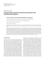
3.1. Experimental Recordings. Figure 1 shows the three
microphone distributions used. All geometries include 16
omnidirectional microphones (Behringer ECM8000) with
the FOV being a 3 m by 3 m plane 1.57 m above the floor. The
FOV plane was spatially sampled at 4 cm increments in the X
and Y directions. Signals were amplified with Audio Buddy
preamplifiers and sampled with two 8-channel Delta 1010
digitizers at 22.05 kHz (both manufactured by M-Audio,
Irwindal, CA) and downsampled to 16 kHz for processing.
Figure 1(a) shows a schematic of the linear array placed
1.52 meters above the floor, 0.5 m away from the FOV
edge. The linear microphone spacing was 0.23 m in this
case. The array was symmetrically placed along the y-axis
relative to the FOV. Figure 1(b) shows a perimeter array with
microphones placed 1.52 meters above the floor, 0.5 m away
from the FOV plane, and a microphone spacing of 0.85 m
along the perimeter. Figure 1(c) shows the planar array with
microphones placed in a plane 1.98 m above the ground in


EURASIP Journal on Advances in Signal Processing

5

2.5
2
1.5
Z

2
1

2
Z 1
0

0
1

−1

0

−1

Y

1
0.5

Z 1
1

X

0
1

0
Y

(a)

0 X
−1

0
Y

1

0

−1

−1

(b)

−1

0
X

1

(c)

Figure 1: Microphone distributions and FOV (shaded plane) for simulation and experimental recordings with axes in meters. Small filled
circles outside the FOV denote a microphone position, and the square and star markers in the FOV denote the smallest and largest (resp.)
differential path distance standard deviation over all pairs: (a) linear, (b) perimeter, and (c) planar.

a rectangular grid starting on a corner directly above the FOV
with a microphone spacing of 1 m in the X and Y directions.
Aluminum struts around the FOV held the microphones
in place, and positions were measured manually multiple
times with a laser meter and tape measure. Precision limits
of the measurements were estimated to be within ±2 cm.
Sound speeds were measured on the day of each recording,
which was 347 m/s for the linear array and 346 m/s for the
perimeter and planar arrays. Two speakers (Yamaha NS-E60
speakers) were paced outside the FOV approximately 2 m
away from the FOV to act as white noise sources and create
a nonstationary power distribution over the FOV. Relative
to the geometries shown in Figure 1, the noise sources were
placed beyond the negative X and negative Y axes.
Five separate recordings of 25 seconds each were made
for the microphone geometries, and the white noise signals
were varied for each recording. The SRCP images were
created with the algorithm based on (7), where signals were
partitioned into 20 ms segments (Δl ) and incremented every
10 ms to create a sequence of the SRCP images. Scale values
for the CFAR thresholds were estimated from the absolute
values of negative pixels within a 15 × 15 neighborhood
about the center (test) pixel. This resulted in a total of 46.5

million detection tests for estimating the FA probabilities.
Various levels of high-pass filtering and partial whitening
were applied before creating the SRCP images and testing
CFAR performance. The level of partial whitening was
controlled with the parameter β in (3).
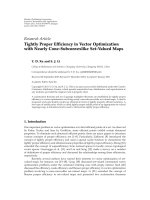
3.2. Differential Path Length Analysis. In order to determine
the distributions of microphone differential path lengths,
normalized histograms (compute from 240 microphone
pairs for each FOV point) were plotted for two particular
FOV positions corresponding to the maximum and minimum standard deviations. These positions are indicated
with the square (minimum) and star (maximum) markers
on the FOVs in Figure 1. Figure 2 shows the normalized
histograms of the microphone differential path lengths and

standard deviations for these points. Visual observation
suggests the distributions are similar to Gaussian in that
they have a central tendency, but they are also like the
uniform distribution in their limited support. The uniform
distribution results in a more conservative performance
and represents a worse case, since the mean offset rolls off
faster for the Gaussian assumption in (13) than that for
the uniform assumption in (14). Therefore, the uniform
distribution is used in the analyses to determine frequency
limits for the acoustic sources based on array properties.
Based on empirical observations, it was determined that
frequencies larger than the third null of the sinc function
(which are limited to −20 dB or less from the maximum)
typically result in good CFAR performance. Thus, highpass filtering the signal at this limit, or reducing their
relative high-frequency contribution with the PHAT, reduces
the low-frequency signal component contributions that the

microphone distribution cannot properly decorrelate. Using
the third null of the sinc function, the low-frequency limit
can be computed from
fL =

3c
√ ,
σΔ 12

(15)

where c is the sound speed and σΔ is the standard deviation
of the differential path lengths. For the linear, perimeter, and
planar geometries, the lower frequency limits corresponding
to the minimum standard deviations over the FOV are
1435 Hz, 790 Hz, and 447 Hz, respectively. These limits
correspond to the worst-case position over the FOV. For a
prediction of an average performance for the microphone
geometry, the median of the standard deviations can be used.
For the linear, perimeter, and planar geometries the median
values are .61, 1.25, and 1.13 respectively, and correspond to
frequency limits of 493 Hz, 240 Hz, and 266 Hz. The impact
of these limits on CFAR performance will be investigated in
the next 2 sections.


6

EURASIP Journal on Advances in Signal Processing

1

1

1

0.8

0.8

0.8

0.6

0.6

0.6

0.4

0.4

0.4

0.2

0.2

0.2

0

−5

0
(meters)

5

0

−5

0
(meters)

5

0

−5

0
(meters)

σmin = 0.21
σmax = 1.42

σmin = 0.38
σmax = 1.88

σmin = 0.67
σmax = 1.48

(a)

(b)

5

(c)

Figure 2: Normalized histograms for microphone pair differential path lengths at FOV points that generate the minimum and maximum
standard deviations for (a) linear geometry, (b) perimeter geometry, and (c) planar geometry.

4. Coherent Power Distribution Analysis
This section examines the noise-only distributions for the
positive and negative coherence values in a test neighborhood. Histograms were created by normalizing nonoverlapping 15 × 15 pixel neighborhoods by the root-mean
square of the negative pixel values to reduce the effects
of the nonstationary noise power over the SRCP images.
Normalized coherent power values were binned over values
ranging from 0 to 15 with 0.0125 intervals. The cumulative
distribution functions (cdfs) were estimated from the normalized histograms, and the cdf complements (1-cdf) were
plotted on a log scale to examine distribution tail differences
between the positive and negative pixel absolute values. The
complement cdf corresponds directly to the FA probability as
a function of threshold.
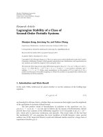
Figure 3 compares the cdf complements of the positive
and negative SRCP values for all geometries with two levels
of high-pass filtering. The distances between the curves

along the x-axis correspond to the error in the threshold
estimation between the positive and negative pixels values.
The relative deviations from symmetry, observed in Figure 3,
are consistent with differential path length analyses of the
previous section. The linear geometry exhibits the largest
deviation from symmetry, while the perimeter and planar
distributions are much less. A high-pass filter with cutoff
frequency at 300 Hz was applied for the results shown in
Figures 3(a), 3(c), and 3(e). For the planar and perimeter
geometries, the cutoff frequency is higher than the lower
limit required by (15) based on the median standard
deviation (266 Hz for planar and 240 Hz for perimeter), but
the 300 Hz cutoff was less than the lower frequency limit
for the linear geometry (493 Hz). Figures 3(b), 3(d), and
3(f) show the corresponding results for a 1500 Hz high-pass
filter cutoff which corresponds to frequencies greater than
the minimum standard deviation for all geometries (for the
linear geometry, this corresponded to 1435 Hz). Minimal
improvements result for the planar and perimeter geometries

because 300 Hz was sufficient, while symmetry significantly
improved for the linear geometry.
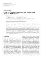
Figure 4 is analogous to Figure 3 with the addition of
the PHAT (total whitening) being applied to the microphone channels. An overall improvement in symmetry is
observed for all cases. The best symmetry is achieved for
the perimeter array, with little improvement resulting from
high-pass filtering at 1500 Hz (Figure 4(d)), since the highfrequency emphasis of the PHAT sufficiently reduced the
impact of the lower frequencies. The linear geometry shows
the most dramatic improvement as a result of high-pass
filtering at 1500 Hz (Figures 4(a) and 4(b)) and the PHAT

operation. Reasonable symmetry on the order of the other
two geometries is achieved for the linear array in this case.
Finally, data were modeled with a Weibull distribution
with cdf given by
P(Sc ) = 1 − exp

Sc
a

b

,

(16)

where a and b are the scale and shape parameters, respectively. A maximum likelihood estimate of the Weibull parameters was performed on the SRCP image pixels (positive
and negative values separately). These estimates provided
an approximate range of shape parameters for the CFAR
algorithm applied in the next section. Table 1 shows the
shape parameter estimates for the two levels of filtering
and three whitening levels. While total whitening results
in the best distribution symmetry, previous work [11, 12,
16] showed that significantly better detection rates are
achieved with partial whitening, rather than total whitening.
Therefore, partial whitening results with β = 0.75 are also
included in the table.

5. CFAR Performance Results and Discussion
This section describes the CFAR threshold estimation and
tests its performance. Based on the differences between

EURASIP Journal on Advances in Signal Processing

10−2
10−3
10−4
10−5
10−6
10−7

0

2

4

6 8 10
Threshold

10−2
10−3
10−4
10−5
10−6
10−7

12 14

10−1

False-alarm probability

10−1
False-alarm probability

False-alarm probability

10−1

7

0

2

4

(a)

10−3
10−4
10−5
10−6
4

10−5
10−6
0

2

4

6 8 10
Threshold

12 14

12 14

(c)

10−2
10−3
10−4
10−5
10−6
10−7

6 8 10
Threshold

10−1
False-alarm probability

False-alarm probability

False-alarm probability

10−2

2

10−4

10−7

12 14

10−1

0

10−3

(b)

10−1

10−7

6 8 10
Threshold

10−2

0

2

4

6 8 10
Threshold

12 14

10−2
10−3
10−4
10−5
10−6
10−7

0

2

4

6 8 10
Threshold

Positive values
Negative values

Positive values
Negative values

Positive values

Negative values

(d)

(e)

12 14

(f)

Figure 3: Cumulative distribution function complements for positive and negative SRCP values estimated from experimental data with
high-pass filtering (a) linear array, 300 Hz cutoff (b) linear array, 1500 Hz cutoff (c) perimeter array, 300 Hz cutoff (d) perimeter array,
1500 Hz cutoff (e) planar array, and 300 Hz cutoff (f) planar array, 1500 Hz cutoff.

Table 1: Weibull parameter estimates for coherent power.
Filter cutoff (Hz)

Geometry

Linear

300

Perimeter

Planar

Linear

1500

Perimeter

Planar

β

Shape parameter (b)
Positive values
Negative values

% Difference

0
0.75
1
0
0.75
1
0
0.75
1

0.52
0.67
0.98
1.16
1.19
1.20
1.17

1.16
1.17

1.69
1.44
1.36
1.36
1.30
1.29
1.36
1.32
1.32

106
73
33
16
9
7
15
13
12

0
0.75
1
0
0.75
1
0

0.75
1

1.07
1.16
1.19
1.18
1.20
1.21
1.17
1.17
1.18

1.43
1.33
1.32
1.36
1.30
1.29
1.36
1.31
1.31

29
14
11
14
8
7
15

11
10


8

EURASIP Journal on Advances in Signal Processing

10−2
10−3
10−4
10−5
10−6
10−7

0

2

4

6 8 10
Threshold

10−2
10−3
10−4
10−5
10−6
10−7

12 14

10−1
False-alarm probability

10−1
False-alarm probability

False-alarm probability

10−1

0

2

4

(a)

10−3
10−4
10−5
10−6
4

10−5
10−6
0

2

4

6 8 10
Threshold

12 14

10−1

10−2
10−3
10−4
10−5
10−6
10−7

12 14

6 8 10
Threshold
(c)

False-alarm probability

False-alarm probability

False-alarm probability

10−2

2

10−4

10−7

12 14

10−1

0

10−3

(b)

10−1

10−7

6 8 10
Threshold

10−2

0

2

4

6 8 10
Threshold

12 14

10−2
10−3
10−4
10−5
10−6
10−7

0

2

4

6 8 10
Threshold

Positive values
Negative values

Positive values
Negative values

Positive values
Negative values

(d)

(e)

12 14

(f)

Figure 4: Cumulative distribution function complements for positive and negative SRCP values estimated from experimental data with
high-pass filtering and whitening with the PHAT (a) linear array, 300 Hz cutoff (b) linear array, 1500 Hz cutoff (c) perimeter array, 300 Hz
cutoff (d) perimeter array, 1500 Hz cutoff (e) planar array, and 300 Hz cutoff (f) planar array, 1500 Hz cutoff.

the distributions shown in the last section, a reasonable goal
for good performance is to have FA probabilities remain
within an order of magnitude of the desired FA probability
over a broad range of desired FA probabilities (10−6 to 10−1 ).
5.1. CFAR Threshold Estimation and Results. The Weibull
distribution was used primarily for its ability to model
skewness via its shape parameter. The shape parameter,
b, was selected based on the limited ranges shown in
Table 1. Therefore, given a known shape parameter, the scale
parameter is computed from the negative coherent power
values via maximum likelihood estimate
⎛

1

a=⎝ −
N0

⎞1/b
b

| Si | ⎠

,

(17)

−
Si ∈N0

where Si are the coherent powers in test pixel neighborhood
−
set, N0 , with subset N0 denoting only the negative coherent
−
−
power values, and N0 denotes the number of pixels in N0 .
For a user specified FA probability, PFA , the test threshold is
computed through the inverse compliment cdf of(16)
T = a[− ln(PFA )]1/b ,

(18)

where PFA is the desired FA probability. The local-scale
values for each test pixel are computed and substituted

into (18) to compute the thresholds for each neighborhood.
Experimental FA probabilities are computed as the number
of times the test pixel value exceeds the threshold, divided by
the total number of test points (46.4 million test points).
For the linear geometry, Figure 5 presents the ratio of
experimental to desired FA probabilities versus the desired
FA probabilities. The broken line on the plots is at a ratio
of one, indicating an agreement between experimental and
desired FA probabilities (target performance). Figure 5(a)
shows differences larger than one order of magnitude
between the desired and experimental FA probabilities for
shape parameter b = 1.26, and while some improvement
is observed in Figure 5(b) as a result of selecting a lower
b (increased skewness), the best performance with cutoff
frequency of 300 Hz corresponds to b = 0.6. The ratios, however, still exceed an order of magnitude over the desired FA
probability range. Thus, as the previous analysis predicted,
the linear distribution has poor CFAR performance due to
its limited differential microphone path differences.
To demonstrate the impact of the lower frequencies on
this performance, the signals are high-pass filtered with a
cutoff of 1500 Hz. These results are presented in Figure 6.
Note in Figure 6(a) that while the error is reduced over the
cases shown in Figure 5, significant error still exists without
whitening from the PHAT; however, with whitening, the
FA probability ratios stay within one order of magnitude.


EURASIP Journal on Advances in Signal Processing

9

102

101

101

Desired to experimental FA ratio

Desired to experimental FA ratio

102

100
10−1
10−2
10−3
10−4
10−6

10−5

10−4
10−3
Desired FA probability

10−2

100
10−1
10−2

10−3
10−4
10−6

10−1

β=0
β = 0.85
β=1

10−5

10−4
10−3
Desired FA probability

10−2

10−1

b = 0.6
b = 0.9
b = 0.5
(a)

(b)

Figure 5: Ratios of specified to empirical (experimental) FA probabilities for linear array for high-pass filtered signals with cutoff frequency
of 300 Hz. (a) Variations of PHAT-β parameters using shape parameter of 1.26, (b) variations of shape parameters using beta equal to 0.85.
102

101

101

Desired to experimental FA ratio

Desired to experimental FA ratio

102

100
10−1
10−2
10−3
10−4
10−6

10−5

10−4
10−3
Desired FA probability

β=0
β = 0.75

10−2

10−1

β = 0.85
β=1
(a)

100
10−1
10−2
10−3
10−4
10−6

10−5

10−4
10−3
Desired FA probability

10−2

10−1

b = 1.2
b = 1.26
b = 1.3
(b)

Figure 6: Ratios of specified to empirical (experimental) FA probabilities for linear array for high-pass filtered signals with cutoff frequency
of 1500 Hz. (a) Variations of PHAT-β parameters using shape parameter of 1.26, (b) variations in shape parameters using beta equal to 0.85.

Figure 6(b) demonstrates the performance sensitivity to the
shape parameter, with the best performance achieved for
shape parameter b = 1.26 and good performance being
maintained over the range from b = 1.2 to 1.3, which is
consistent with the shape parameters shown in Table 1 for
this case.
Figure 7 shows analogous results for the perimeter
distribution. The previous analysis indicated lower frequency
limits of 240 Hz and 790 Hz corresponding to the median
and minimum standard deviations of the differential path

lengths. While results high-pass filtered at 300 Hz satisfy
over 50% of the pixels in the FOV, sufficient pixels existed
requiring a higher cutoff frequency to impact the CFAR
performance. Rather than increasing the cutoff as in the
previous example, whitening was used to create a highfrequency emphasis to minimize the impact of these pixels.
Note that Figure 7(a) shows that b = 1.26 results in
good CFAR performance provided a whitening operation is
applied. Figure 7(b) shows a slight improvement when b is
increased to 1.3.


10

EURASIP Journal on Advances in Signal Processing
102

101

101

Desired to experimental FA ratio

Desired to experimental FA ratio

102

100
10−1
10−2
10−3
10−4
10−6

10−5

10−4
10−3
Desired FA probability

β=0
β = 0.75

10−2

100
10−1
10−2
10−3
10−4

10−6

10−1

β = 0.85
β=1

10−5

10−4
10−3
Desired FA probability

10−2

10−1

b = 1.26
b = 1.3

(a)

(b)

Figure 7: Ratios of specified to empirical (experimental) FA probabilities for perimeter array for high-pass filtered signals with cutoff
frequency of 300 Hz. (a) Variations in PHAT-β parameters using shape parameter of 1.26, (b) variations in shape parameters using beta
equal to 0.85.

102

101

101

Desired to experimental FA ratio

Desired to experimental FA ratio

102

100
10−1
10−2
10−3
10−4
10−6

10−5

10−4
10−3
Desired FA probability

10−2

10−1

β=0
β = 0.85
β=1

100
10−1
10−2
10−3
10−4
10−6

10−5

10−4
10−3
Desired FA probability

10−2

10−1

β=0
β = 0.85
β=1
(a)

(b)

Figure 8: Ratios of specified to empirical (experimental) FA probabilities for planar array for high-pass filtered signals with cutoff frequency
of 300 Hz. (a) Variations in PHAT-β parameters using shape parameter of 1.26, (b) variations in PHAT-β parameters, using shape parameter
of 1.12.

Results for the planar geometry are shown in Figure 8.

In comparing Figures 7(a) and 8(a), the perimeter array
shows superior CFAR performance, whereas whitening does
not have an observable impact on CFAR performance for
the planar distribution. The previous analysis showed a
266 Hz limit and a 447 Hz limit based on the median
and minimum standard deviation, which is a more limited
frequency range compared to the perimeter distribution,

thus, explaining its performance being less sensitive to
whitening. To improve performance, the high-pass filter
can be set higher (i.e., to 500 Hz), but this has practical
disadvantages in that a significant amount of the signal
power can exist below this cutoff. An alternative approach
to compensate for the increased skewness is to decrease the
Weibull shape parameter. Figure 8(b) shows the result of
dropping b to 1.12, which is lower than the positive coherent


EURASIP Journal on Advances in Signal Processing
power terms for this case shown in Table 1. While the error
varies nonuniformly over the range tested, it remains within
one order of magnitude.
5.2. Discussion of Results. Overall, results show that the
perimeter array has the best performance in that it is least
sensitive to lower frequencies. The high-pass filtering with
a cutoff of 300 Hz and partial whitening result in improved
performance over the whole FOV. In general, performance
is improved for higher frequency sources; however, raising
the high-pass filter cutoff frequency can reduce target
detection sensitivity, so the other approaches are usually

more desirable, such as whitening or adjusting the statistical
models.
The linear and planar distributions did not perform
as well as the perimeter distribution, as predicted by their
differential path length standard deviations. In both cases,
performance was improved by using a more skewed Weibull
distribution to fit the data (Figures 5(b) and 8(b)). The
increased distribution skewness compensates for some of the
performance losses due to the nonsymmetries. In selecting
a more skewed b value for negative pixels, a larger-scale
parameter estimate from (17) will result (for the same data).
This bias increases the threshold, which compensates for the
high levels of positively skewed values. This approach is limited in that if the shape parameters deviate too far from the
actual data properties, consistent CFAR performance cannot
be maintained over the range of desired FA probabilities. This
was the case for the results shown in Figure 5.
Whitening is an important operation for reducing the
noise distribution skewness as shown by comparing Figures
3 and 4. Especially note that the distribution of the negative
coherent power values does not change much as a result of
whitening; however, there is a much larger reduction in skewness for the positive coherent power points. This partially
explains why the PHAT improves SRP image appearance.
The impulse/speckle noise resulting from the highly skewed
noise pixels tends to create a distracting background from
which to visually identify targets. The other advantage
of whitening is that it reduces the correlation between
adjacent pixels by emphasizing the higher frequencies. The
increased spatial decorrelation or reduced correlation length
for higher frequencies is indicated by the mic-distribution
and noise-path factors of (12). Smaller wavelengths increase

the sensitivity of the phase to changes in the differential path
lengths as a result of spatial changes in the FOV. This not
only improves noise distribution symmetry, but effectively
increases the uncorrelated negative (noise) pixels in the test
point neighborhood, which can reduce variations in the
Weibull-scale parameter estimate.
For examples presented in this paper, a 15 × 15 pixel
neighborhood was used. Other sizes also were examined
(such as 7 × 7), and the 15 × 15 did the best as far as
being the smallest neighborhood to achieve nearly the best
performance for all three microphone arrays. One possible
explanation for the poor performance of the linear array
is that the neighborhood size was not large enough for
good convergence of a. Experimental results (not shown

11
here) indicated that the linear array was more sensitive
to the neighborhood size than the planar and perimeter
distribution. A neighborhood of size 7 × 7 severely degrades
the performance in the linear array. The CFAR performance
for the planar and perimeter still remained within an order
of magnitude for the 7 × 7 pixel neighborhood. However,
increases in neighborhood size only resulted in incremental
improvements for all arrays and eventual degradation due to
the nonstationarity of the noise. So while the neighborhood
size and limited correlation length of the linear array did
contribute to its poor performance, the greater factor was the
distribution skewness, as observed in Figures 3 and 4.
The standard deviations of the differential path lengths
predicted the relative CFAR performance of the different

microphone geometries. The frequency limits for each array
as computed by (15) predicted the low-frequency limits with
reasonable accuracy. For the linear array, however, these
predictions were not as good. Acceptable performance for
the linear distribution was not quite achieved by high-pass
filtering at 1500 Hz, which is greater than to the frequency
required by its worst case FOV point (1435 Hz). Whitening
was still required after this filtering for acceptable CFAR
performance. This was in part due to not taking the noisepath factor into account.
The noise-path factor depends on the path lengths from
the noise sources to the microphones and can vary as sources
move in the environment. For this paper, however, the noise
sources were stationary. For the linear array, one noise source
was positioned broadside, nearly 5 m away. This resulted in
a small differential path length variance and significantly
reduced the decorrelation from noise-path factors in the
summations. The perimeter and planar geometries had more
endfire-like orientations to both major noise sources, thereby
increasing the differential path variance for the noise-path
factors and making it less of a factor in the performance. As a
result, the shape parameters for fitting the Weibull distribution to the planar and perimeter coherent noise values were
very close to the 1.26 (expected for Gaussian noise), whereas
the linear geometry shape parameters deviated much more
from the 1.26 level, even after high-pass filtering at 1500 Hz.

6. Conclusion
This paper introduced a method for CFAR threshold estimation that uses the negative coherent power values in images
created with SRP algorithms. Reasonable performance was
obtained provided the source content was above the lower
frequency limit associated with the array. An analysis based

on differential path lengths was used to predict relative CFAR
performance between microphone distribution geometries
based on the source frequency limit. It was shown that
good CFAR performance could be obtained for microphone
arrays with large differential path length variations over all
microphone pair combinations relative to the signal source
wavelengths. The analysis requires a standard deviation
computation of the differential path lengths between microphone pairs and FOV points, which can be done for any


12
geometry and is especially useful for systems with irregularly
positioned microphones and FOV regions.

Acknowledgment
This work was supported in part by the National Science
Foundation EPSCoR Program (Award 0447479).

References
[1] J. L. Flanagan, D. A. Berkley, G. W. Elko, J. E. West, and M.
M. Shondhi, “Autodirective microphone systems,” Acoustica,
vol. 73, pp. 58–71, 1991.
[2] F. Khalil, J. P. Jullien, and A. Gilloire, “Microphone array for
sound pickup in teleconference systems,” AES: Journal of the
Audio Engineering Society, vol. 42, no. 9, pp. 691–700, 1994.
[3] C. Che, M. Rahim, and J. Flanagan, “Robust speech recognition in a multimedia teleconferencing environment,” Journal
of the Acoustical Society of America, vol. 92, no. 4, p. 2476, 1992.
[4] D. Giuliani, M. Omologo, and P. Svaizer, “Talker localization
and speech recognition using a microphone array and a crosspower spectrum phase analysis,” in Proceedings of the International Conference on Spoken Language Processing (ICSLP ’94),
vol. 3, pp. 1243–1246, September 1994.

[5] T. B. Hughes, H. S. Kim, J. H. Dibiase, and H. F. Silverman,
“Performance of an HMM speech recognizer using a real-time
tracking microphone array as input,” IEEE Transactions on
Speech and Audio Processing, vol. 7, no. 3, pp. 346–349, 1999.
[6] H. F. Silverman, “Some analysis of microphone arrays for
speech data acquisition,” IEEE Transactions on Acoustics,
Speech, and Signal Processing, vol. 35, no. 12, pp. 1699–1712,
1987.
[7] S. M. Yoon and S. C. Kee, “Speaker detection and tracking
at mobile robot platform,” in Proceedings of the International
Symposium on Intelligent Signal Processing and Communication
Systems (ISPACS ’04), pp. 596–600, November 2004.
[8] T. S. Huang, “Multimedia/multimodal signal processing, analysis, and understanding,” in Proceedings of the 1st International
Symposium on Control, Communications and Signal Processing,
p. 1, 2004.
[9] J. H. DiBiase, H. F. Silverman, and M. S. Brandstein, “Robust
localization in reverberant rooms,” in Microphone Arrays,
Signal Processing Techniques and Applications, pp. 157–180,
Springer, New York, NY, USA, 2001.
[10] T. Gustafsson, B. D. Rao, and M. Trivedi, “Source localization
in reverberant environments: modeling and statistical analysis,” IEEE Transactions on Speech and Audio Processing, vol. 11,
no. 6, pp. 791–803, 2003.
[11] K. D. Donohue, J. Hannemann, and H. G. Dietz, “Performance of phase transform for detecting sound sources with
microphone arrays in reverberant and noisy environments,”
Signal Processing, vol. 87, no. 7, pp. 1677–1691, 2007.
[12] A. Ramamurthy, H. Unnikrishnan, and K. D. Donohue,
“Experimental performance analysis of sound source detection with SRP PHAT-β,” in Proceedings of the IEEE Southeastcon, pp. 422–427, March 2009.
[13] H. Rohling, “Radar CFAR thresholding in clutter and multiple
target situations,” IEEE Transactions on Aerospace and Electronic Systems, vol. 19, no. 4, pp. 608–621, 1983.
[14] K. D. Donohue and N. M. Bilgutay, “OS characterization for

local CFAR detection,” IEEE Transactions on Systems, Man and
Cybernetics, vol. 21, no. 5, pp. 1212–1216, 1991.

EURASIP Journal on Advances in Signal Processing
[15] S. Kuttikkad and R. Chellappa, “on-Gaussian CFAR techniques for target detection in highresolution SAR images,
image processing,” in Proceedings of the IEEE International
Conference on Image Processing (ICIP ’94), vol. 1, pp. 910–914,
November 1994.
[16] K. D. Donohue, K. S. McReynolds, and A. Ramamurthy,
“Sound source detection threshold estimation using negative
coherent power,” in Proceedings of the SouthEast Conference,
pp. 575–580, April 2008.