Báo cáo hóa học: " Research Article A Complexity-Reduced ML Parametric Signal Reconstruction Method" pptx

Hindawi Publishing Corporation
EURASIP Journal on Advances in Signal Processing
Volume 2011, Article ID 875132, 14 pages
doi:10.1155/2011/875132
Research Article
A Complexity-Reduced ML Parametr ic Signal
Reconstruction Method
Z. Deprem,
1
K. Leblebicioglu,
2
O. Arıkan,
1

and A. E. C¸etin
1
1
Department of Electrical and Electronics Engineering, Bilkent University, Bilkent, Ankara, 06800, Turkey
2
Department of Electrical and Electronics Engineering, Middle East Technical University, Ankara, 06531, Turkey
CorrespondenceshouldbeaddressedtoZ.Deprem,
Received 2 September 2010; Revised 8 December 2010; Accepted 24 January 2011
Academic Editor: Athanasios Rontogiannis
Copyright © 2011 Z. Deprem et al. This is an open access article distributed under the Creative Commons Attribution License,
which permits unrestricted use, distribution, and reproduction in any medium, provided the original work is properly cited.
The problem of component estimation from a multicomponent signal in additive white Gaussian noise is considered. A parametric

ML approach, where all components are represented as a multiplication of a polynomial amplitude and polynomial phase term, is
used. The formulated optimization problem is solved via nonlinear iterative techniques and the amplitude and phase parameters
for all components are reconstructed. The initial amplitude and the phase parameters are obtained via time-frequency techniques.
An alternative method, which iterates amplitude and phase parameters separately, is proposed. The proposed method reduces
the computational complexity and convergence time significantly. Furthermore, by using the proposed method together with
Expectation Maximization (EM) approach, better reconstruction error level is obtained at low SNR. Though the proposed method
reduces the computations significantly, it does not guarantee global optimum. As is known, these types of non-linear optimization
algorithms converge to local minimum and do not guarantee global optimum. The global optimum is initialization dependent.
1. Introduction
In many practical signal applications involving ampli-
tude and/or phase-modulated carrier signals, we encounter
discrete-time signals which can be represented as

s
[
n
]
= a
[
n
]
e
j∅[n]
,(1)
where a[n]and

∅[n] are the real amplitude and phase
functions, respectively. Such signals are common in radar,
sonar applications, and in many other natural problems. A
multicomponent [1] signal is a linear combination of these
types of signals and is given by
s
[
n
]
=
L


i=1
a
i
[
n
]
e
j∅
i
[n]
,(2)
where s

i
[n] = a
i
[n]e
j∅
i
[n]
is the ith component and L is the
number of components. Clearly, the linear decomposition
of the multicomponent signal in terms of such components
is not unique. Some other restrictions should be put on
the components to have a unique decomposition [1]. In

general, a component is the part of the multicomponent
signal which is identifiable in time, in frequency, or in mixed
time-frequency plane. Therefore, we will assume that the
different components are well separated in time-frequency
plane and have a small instantaneous bandwidth compared
to separation between components.
The main problem is to separate the components from
each other or to recover one of the components. In general
the approaches for the solution are those which use non-
parametric time-frequency methods and those of parametric
ones. In case where the desired signal component is separable
or disjoint in one of time or frequency domain, then, with

some sort of time or frequency masking, the component can
be estimated. When the signals are disjoint either in time
or in frequency domain, then time-frequency processing
methods are needed for component separation. But, in some
cases even though the components are not separated in time
or in frequency, the Fractional Fourier Transform [2–4]can
be used to separate the components at the fraction, where
they are disjoint.
Time Frequency Distribution- (TFD-) based waveform
reconstruction techniques, for example, the one in [5],
2 EURASIP Journal on Advances in Signal Processing
synthesize a time-domain signal from its bilinear TFD. In

these algorithms, a time-domain signal whose distribution is
close to a valid TFD, in a least-squares sense, is searched for.
The well-known time-frequency method is the Wigner-
Distribution [6] based signal synthesis [5, 7–9]. The main
drawback related to time-frequency methods is the cross-
terms and resolution of the time-frequency representations
[10]. Therefore, there have been many efforts to obtain cross-
term-free and high-resolution TFDs [11–13].
In parametric model a signal or component is repre-
sented as a linear combination of some known basis func-
tions [14, 15], and the component parameters are estimated.
In many radar and sonar applications the polynomials are

good basis functions.
If the phase and amplitude functions in (1)arepoly-
nomials and amplitude function is constant or slowly
varying, the Polynomial Phase Transform (PPT) [14, 16]is
a practical tool for parameter estimation. While the method
is practical, it has difficulties in time-varying amplitude and
multicomponent cases [17]. It is also suboptimal since the
components are extracted in a sequential manner.
Another solution is the ML estimation of the parameters.
The related method is explained in [15, 17]. The ML esti-
mation of the parameters requires a multivariable nonlinear
optimization problem to be solved. Therefore, the solu-

tion requires iterative techniques like nonlinear conjugate
gradient (NL-CG) or quasi-Newton-type algorithms and is
computationally intensive [15, 17]. Another requirement is
a good initial estimate which avoids possible local minima.
But it estimates all parameters as a whole and is optimal in
this respect. Also it does not suffer from cross-terms related
to time-frequency techniques.
In [14] an algorithm is explained which extracts the
components using PPT in a sequential manner. In [18]a
mixed time-frequency and PPT-based algorithm is proposed.
The examples with the ML approach are given in [15, 17].
In this paper a method is proposed which uses ML

estimation. Similar to [18], the initial estimates are obtained
from time-frequency representation of the multicomponent
signal and then all parameters are estimated by ML estima-
tion. Since ML estimation requires large amount of computa-
tion, a method is proposed to reduce the computations. The
proposed method iterates amplitude and phase parameters
separately by assuming that the other is known. The method
is different from the ones given in [15, 17], where the
amplitude parameters are eliminated analytically and the
resultant equivalent cost function is minimized.
Eliminating amplitude parameters analytically results in
a cost function which has less number of parameters. But

it is computationally more complex in terms of function
and gradient evaluations, which are needed in nonlinear
optimization iterations.
With the proposed method, since the cost functions for
separate amplitude and phase parameters are less complex,
the amount of computation is reduced compared to case
where amplitude parameters are eliminated analytically. Fur-
thermore, by using the proposed method in an expectation
maximization loop, a better reconstruction error level is
obtained. The results are verified with simulations.
In Section 2 we describe the notation and give the
explanation of the ML estimation approach which is given

in [15]. In Section 3 we describe the proposed method.
In
Section 4 we compare the computational cost of the
proposed method with the case where amplitude parameters
are eliminated analytically. In Section 5 we give a brief expla-
nation of Expectation Maximization (EM) and how to use
the proposed alternating phase and amplitude minimization
method in an EM loop. In Section 6 we drive the Cramer-
Rao Bounds on mean square error related to component
reconstruction. In Section 7 we present the simulation
results. First taking Cramer-Rao bounds as the reference we
compare the proposed method with the one given in [15]in

terms of mean square reconstruction error and then compare
their performance in terms of computational cost.
2. Problem Formulation and ML Estimation
Let x[n] be a discrete-time process consisting of the sum of
a deterministic multicomponent signal and additive white
Gaussian noise given by
x
[
n
]
=
L


i=1
a
i
[
n
]
e
j∅
i
[n]
+ w

[
n
]
, n = 0, 1, , N −1
,(3)
where w[n] is the complex noise process. Denoting g
k
[n]and
p
k
[n] as the real-valued basis functions for amplitude and
phase terms, respectively, we will have

a
i
[
n
]
=
P
i

k=0
a
i,k

g
k
[
n
]
,(4)
∅
i
[
n
]
=

Q
i

k=0
b
i,k
p
k
[
n
]
,(5)

where a
i,k
and b
i,k
are the real valued amplitude and phase
coefficients for the ith component. Similarly P
i
+1and
Q
i
+ 1 are the number of coefficients for amplitude and
phase functions of the ith component. In general, basis

functions can be any functions which are square integrable
and spans the space of real and integrable functions in a given
observation interval. Also they can be selected to be different
for amplitude and phase and for each component. In this
paper they are assumed to be polynomial for both amplitude
and phase and for all components. Therefore, P
i
and Q
i
corresponds to orders for amplitude and phase polynomials
of the ith component, respectively.
Defining the amplitude and phase coefficients of the ith

component by the vectors
a
i
=

a
i,0
a
i,1
a
i,2
··· a

i,P
i

T
,
b
i
=

b
i,0
b

i,1
b
i,2
··· b
i,Q
i

T
,
(6)
we can define parameter vectors for all the components as
a

=

a
T
1
a
T
2
a
T
3
··· a

T
L

T
,
b
=

b
T
1
b

T
2
b
T
3
··· b
T
L

T
.
(7)

EURASIP Journal on Advances in Signal Processing 3
We will use the following notation
x
= x
[
n
]
=

x
[
0

]
x
[
1
]
x
[
2
]
··· x
[
N − 1

]

T
,
(8)
where
n
=
[
0, 1, 2, , N
−1
]

T
,
w
= w
[
n
]
=

w
[
0

]
w
[
1
]
w
[
2
]
··· w
[
N − 1

]

T
,
e
j∅
i
[n]
=

e
j∅

i
[0]
e
j∅
i
[1]
e
j∅
i
[3]
··· e
j∅

i
[N−1]

T
,
(9)
where the bold characters n, x, w,ande
j∅
i
[n]
are all N × 1
vectors. With these definitions the following matrices can be

defined
Φ
i
=

g
0
[
n
]
•e
j∅

i
[n]
g
1
[
n
]
•e
j∅
i
[n]
g

2
[
n
]
•e
j∅
i
[n]
··· g
P
i
[

n
]
•e
j∅
i
[n]

,
(10)
Φ
=
[

Φ
1
Φ
2
Φ
3
···Φ
L
]
, (11)
where “
•”in(10) denotes component-by-component mul-

tiplication of vectors. Φ
i
sareN × (P
i
+1)matriceswhich
contain the phase parameters only and are defined for each
component. The matrix Φ is an N
×

L
i
=1

(P
i
+1)matrix
and again contains the phase parameters for all components.
With these definitions the expression in (3)canbewrittenin
matrix notation as
x
= Φa + w. (12)
In this equation the amplitude parameter vector a enters the
equation in a linear way, while the phase parameter vector b
enters the equation in nonlinear way through Φ.
Now the problem is to estimate combined parameter

vector θ
= [b
T
a
T
]
T
given observed data vector x =

x[0] x[1] x[2] ··· x[N −1]

T

. It is assumed that the
observed data length N is sufficiently greater than the total
number of estimated parameters given by M
=

L
i=1
{(P
i
+
1) + (Q
i

+1)}.
The number of components, since components are
assumed to be well separated on TFD, can be estimated from
TFD. But here we will assume that L is known. Similarly P
i
and Q
i
are assumed to be known. A method to estimate them
can be found in [14, 16].
With the additive white Gaussian noise assumption, the
probability density function (pdf) of data vector x, given the
parameter vector θ and logarithmic likelihood function, is

given by
p
(
x
| θ
)
=
1
(
πσ
2
)

N
exp

−
1
σ
2
x −Φa
2

, (13)
Λ

= log p
(
x | θ
)
=−N
(
ln π +2lnσ
)
−
1
σ
2

x −Φa
2
,
(14)
where σ
2
is the noise variance? Since x and Φ are com-
plex, by defining
x =

Re{x}
T

Im{x}
T

T
and Ψ =

Re{Φ}
T
Im{Φ}
T

T

, the log-likelihood function can be
rewritten in real quantities as
Λ
=−N
(
ln π +2lnσ
)
−
1
σ
2
x −Ψa

2
. (15)
Maximizing log likelihood in (15) corresponds to minimiz-
ing f (a, b)
=x −Ψa
2
.Foragivenphasevectorb, this
cost function is quadratic in amplitude vector a. Therefore,
amplitude vector a can be solved analytically as
a =

Ψ

T
Ψ

−1
Ψ
T
x. (16)
Using this separability feature of the parameter set and
substituting (16)in(15) the original log-likelihood function
can be replaced by
Λ
=−N

(
ln π +2lnσ
)
−
1
σ
2
J
(
b
)
, (17)

where
J
(
b
)
= x
T
P
⊥
Ψ
x, (18)
P

⊥
Ψ
= I − P
Ψ
, (19)
P
Ψ
= Ψ

Ψ
T
Ψ


−1
Ψ
T
. (20)
While the original cost function was a function of a and b,
thisnewaugmentedfunctionisafunctionofb only. Like
the original cost function this new cost function J(b) is also
nonlinear in b. Therefore, minimization requires iterative
methods like nonlinear conjugate gradient or quasi-Newton-
type methods. These iterative methods require also a good
initial estimate to avoid possible local minima. In [15] initial

estimates are obtained by PPT. After b is solved iteratively, a
is obtained by (16).
3. Proposed Method for Iterative Solution
The separability feature of the original cost function in (15)
allows us to reduce the number of unknown parameters
via analytical method. Since the resultant cost function
is just a function of phase parameters, we will call this
method Phase-Only (PO) method. Though PO deals with
reduced set of parameters, the resultant cost function J(b)is
highly nonlinear and more complicated in terms of function
and gradient evaluations. This is a disadvantage when the
minimization of the reduced cost function is to be obtained

via nonlinear iterative methods. Therefore, in this paper,
an alternative method is proposed. The method carries out
two minimization algorithms in an alternating manner. The
method divides the original minimization problem given by
(15) into two subminimizations. The idea is to find one
parameter set assuming that the other set is known. First
assuming that the initial phase estimate

b
0
is known, the cost
function

f
a
(
a
)
= f

a,

b
0


=


x −

Ψ
0
a


2
(21)

4 EURASIP Journal on Advances in Signal Processing
is formed and minimized, and a solution
a
1
is obtained,
where

Ψ
0
is the matrix obtained by initial phase parameter
estimate


b
0
. Then using this amplitude estimate a
1
asecond
cost function
f
b
(
b
)
= f



a
1
, b

=


x
−Ψa
1



2
(22)
is formed and minimized, and a solution

b
1
is found.
These two minimizations constitute one cycle of proposed
algorithm. By repeating this cycle, taking


b
1
as the new
initial phase estimate, the estimates a
2
and

b
2
are obtained.
By repeating the cycles sufficiently many times, the final
estimates

a
∗
and

b
∗
are obtained as shown in

b
0
−→ a
1

−→

b
1
−→ a
2
−→

b
2
−→ a
3

−→

b
3
···a
∗
−→

b
∗
.
(23)

The cost function for amplitude parameters f
a
(a)is
quadratic. Therefore, the solution can be obtained either
analytically or via conjugate gradient (CG). But the cost
function for phase parameters f
b
(b) is nonlinear. Therefore,
we need to use nonlinear methods.
The proposed method, which we will call, from now
on, Alternating Phase and Amplitude (APA) method, is a
generalization of the so-called coordinate descent method

[19], where the minimization of a multivariable function
is done by sequentially minimizing with respect to a single
variable or coordinate and keeping the others fixed. By
cyclically repeating the same process a minimum for the
function is searched. A generalization of coordinate descent
method is the Block Coordinate Descent (BCD) method,
where the variables are separated into blocks containing
more than one variable and the minimization is done over
a block of variables and keeping the others fixed. In our case
we have two blocks, and the minimization over one block
is quadratic. Though the indications on the convergence of
similar algorithms are given in [19], the theoretical proof

regarding the convergence of proposed method is beyond the
scope of this work, and we will content with the simulation
results.
The main trick with proposed algorithm is that during
amplitude and phase minimizations we do not have to
find the actual minimum. What we are looking for is a
sufficient improvement from the current estimate that we
have. Therefore, for the phase iterations rather than iterating
down to the convergence point we can iterate a sufficient
number of iterations to get some improvement. The same
is valid for the minimization of f
a

(a)ifwedecideto
use conjugate gradient. But overall alternating phase and
amplitude iterations will allow us to converge to a minimum.
The first minimization can be chosen to be the minimization
of f
b
(b) instead of f
a
(a). Then the sequence in (23) will start
by
a
0

. The decision about which one to start with should be
based on which initial parameter vector,
a
0
or

b
0
,ismore
close to its actual. This cannot be known in advance, but,
based on success of the method by which the initial estimates
a

0
and

b
0
are obtained, a decision can be given.
Like J(b), f
b
(b) is also nonlinear, and we need iterative
methods like nonlinear conjugate gradient or quasi-Newton.
These methods converge to local minimum and do not
guarantee global minimum unless initial estimates are

sufficiently close to global optimum. Therefore, we need to
find a method which gives us initial estimates. While in
[15] initial estimates are obtained by PPT, in this paper we
obtained the initial estimates from time-frequency methods.
The time-frequency distribution we used is the Short-Time
Fourier Transform (STFT).
At first cycle, the phase iterations will be started by

b
0
=


b
TF
where

b
TF
is the estimate obtained from time-frequency
method. In later cycles, the previous cycle estimates will
be used. If minimization of f
a
(a) is done analytically, then
we will not need any initial value. But, if we decide to use

iterative methods again, we can use initial estimate
a
0
= a
TF
obtained from time-frequency method.
As we stated before we assume that the different compo-
nents are well separated in time-frequency plane and have
a small instantaneous bandwidth; that is, the components
are not crossing each other. Therefore, by using magnitude
STFT, the ridges of each component are detected on TF
plane. The algorithm detects the ridges on TF plane by

detecting local frequency maximums for each time index.
Also by using a threshold the effect of noise is reduced, and
the IF is detected at points where component is stronger
than noise. Therefore, even though when the weak end of
some components is interfering on TF plane with some
other stronger component, the IF of stronger component is
detected at that point, but the week part of other components
is not detected. But the estimates obtained with this method,
though they are not the best ones, will be sufficient as initial
parameters.
Then from the ridges the instantaneous frequency (IF)
samples (


f
i
[n]) for each component are estimated and by
polynomial fit corresponding polynomial is obtained. Then
by integrating this polynomial the phase function

∅
i
[n]
and polynomial coefficients


b
TF
i
for each component are
obtained. By dechirping x[n]bye
−j

∅
i
[n]
and low-pass
filtering the result, the amplitude estimate

a
i
[n] is obtained
for each component. Again by polynomial fit
a
TF
i
is obtained
for each component. The overall steps for the proposed APA
algorithm are summarized in Ta bl e 1.
The initial estimates are obtained from signal TFD by
steps 1–5 given in Ta bl e 1 . Some other methods could also

be used. But in this paper the main focus is on the last
step. Therefore, though the steps 1–5 were implemented, the
efficiency and performance of this part have not been studied
in detail. The only concern was to get initial estimates which
are close enough to actual values to avoid local minima if
possible. But it should be noted that for the comparison
purposes the same initial conditions will be used for the
proposed APA algorithm and the phase-only method given
in [15].
An important issue that we need to question is the
uniqueness of the solution to the optimization problem in
(15). Since we express a component in terms of amplitude

and phase functions and these functions are expressed in
terms of basis functions, we need to question the uniqueness
of the global optimum at three levels.
EURASIP Journal on Advances in Signal Processing 5
Starting form last level, given a phase function
∅
i
[n],
uniqueness of the parameter vector b
i
for this function can
be assured if the base functions p

k
[n], k = 0, 1, ,Q
i
,are
independent of each other. The same is valid for amplitude
function a
i
[n] and parameter vector a
i
.
Uniqueness at the amplitude and phase function level
(model functions level) will not be assured due to phase

ambiguity, because if a
i
[n]and∅
i
[n]constituteacompo-
nent then
−a
i
[n]and∅
i
[n]+π will also constitute the same
component. Therefore, even though a

i
is unique for a
i
[n]
and b
i
is unique for ∅
i
[n], the pair a
i
[n]and∅
i

[n]willnot
be unique for s
i
[n] and, as a result, θ
i
= [b
T
i
a
T
i
]

T
will not
be unique for s
i
[n]. This shows that the global optimum is
not unique in terms of model functions, hence in terms of
parameter vector θ
= [b
T
a
T
]

T
.
On the other hand uniqueness at signal s
i
[n]orcom-
ponent level will be possible if the components are well
separated on TFD [1]. In simple terms if no component is
coinciding at the same time-frequency point with some other
component then the components which constitute the sum
in (2) can be found uniquely. Two extreme cases are those
where all components are separated in time domain or in
frequency domain.

Therefore, even though uniqueness is not satisfied at
model functions level hence at parameter level, it can be
satisfied at component or signal level with the restrictions
on time-frequency plane. In fact, the solution ambiguity
in model or parameter space will not affect the final
performance of the component reconstruction as long as
the combination of model functions or model parameters
gives the same signal or component. In our case we extract
the initial parameters for a component from related TF
area which is disjoint. Therefore, assuming that the initial
parameters are close enough to global optimum, we use
these restrictions, which will make the component level

uniqueness possible, at the beginning.
On the contrary to the assumptions made on time
frequency support of components, in simulations, one
example (Ex2) is selected such that the components are
slightly crossing each other. But most of the parts are
nonoverlapping, and these parts allow estimation of an initial
IF which will help uniqueness, because, we have assumed in
Section 2 that the phase orders Q
i
s are also known. With this
assumption, the set of ambiguous IF estimates hence phase
estimates are eliminated for this example, because fitting

other ambiguous IFs to the known polynomial order will
result in higher fit error. Therefore, for similar examples, the
time-frequency restriction can be slightly relaxed.
3.1. Computational Cost Analysis. With the phase-only
method the resultant cost function J(b)isgivenby(18). For
the sake of computation ease if we reorganize this equation
we will have
J
(
b
)
= x

T
P
⊥
Ψ
x = x
T
x −

Ψ
T
x


T

Ψ
T
Ψ

−1
Ψ
T
x, (24)
where Ψ
= [Ψ

1
Ψ
2
Ψ
3
···Ψ
L
]andΨ
i
is given by
Ψ
i

=
⎡
⎣
Re{Φ
i
}
Im{Φ
i
}
⎤
⎦
=

⎡
⎣
g
0
[
n
]
• Cos
(
∅
i
[

n
]
)
g
1
[
n
]
• Cos
(
∅
i

[
n
]
)
··· g
P
i
[
n
]
• Cos
(

∅
i
[
n
]
)
g
0
[
n
]
• Sin

(
∅
i
[
n
]
)
g
1
[
n
]

• Sin
(
∅
i
[
n
]
)
··· g
P
i
[

n
]
• Sin
(
∅
i
[
n
]
)
⎤
⎦

, (25)
where “•” again denotes component-by-component multi-
plication of vectors.
The gradient of J(b)isgivenby[15]
∇J
(
b
)
=−2x
T
P
⊥

Ψ
B,
(26)
where
B
=
[
B
1
, B
2
, , B

L
]
,
B
i
=


b
i,0
,


b
i,1
,

b
i,2
, ,

b
i,Q
i


,

b
i,k
=
∂Ψ
i
∂b
i,k
R
T
i

x k = 0, 1, , Q
i
,
R
= Ψ

Ψ
T
Ψ

−1
=

[
R
1
, R
2
, , R
L
]
.
(27)
The derivative of Ψ
i

with respect to b
i,k
is computed as
follows:
∂Ψ
i
∂b
i,k
=

Ψ
i

•G
k
, (28)
where

Ψ
i
is the reordered version of Ψ
i
given by

Ψ

i
=

−
Im{Φ
i
}
Re{Φ
i
}

(29)

and G
k
has the same dimensions as

Ψ
i
andateachcolumn
contains the same 2N
×1vector

p
k

[n]
p
k
[n]

. The multiplication
between

Ψ
i
and G
k

is component by component.
With the proposed method, the minimization of f
a
(a)
either by CG or analytically is relatively easy. Similarly the
computation of f
b
(b) =x − Ψa
0

2
is also easy. By defining

z
= Ψa
0
=
L

i=1
z
i
,
z
i

=Ψ
i
a
0
i
=
⎡
⎣
Re{Φ
i
}
Im{Φ

i
}
⎤
⎦

a
0
i
=
⎡
⎣
z

iR
z
iI
⎤
⎦
=
⎡
⎢
⎢
⎢
⎢
⎢

⎢
⎣
P
i

k=0
a
0
i,k
g
k
[

n
]
•Cos
(
∅
i
[
n
]
)
P
i


k=0
a
0
i,k
g
k
[
n
]
•Sin
(

∅
i
[
n
]
)
⎤
⎥
⎥
⎥
⎥
⎥

⎥
⎦
,
(30)
6 EURASIP Journal on Advances in Signal Processing
Table 1: The proposed alternating phase and amplitude (APA) algorithm.
1Compute|STFT| for x[n], and detect the ridges and the number of components L
2Compute

f
i
[n]and


f
i
(t) via polynomial fit
3Compute

∅
i
(t) = 2π

t
0


f
i
(τ)dτ +

∅
i
(0) and

∅
i
[n] determine


b
TF
i
where

∅
i
(0) is the phase offset estimated from data
4Computex[n]e
−j


∅
i
[n]
and low-pass filter to get a
i
[n]
5 Using polynomial fit get
a
TF
i
6 Minimize f
b

(b)and f
a
(a) in an alternating manner using a
0
=

a
TF
and

b
0

=

b
TF
Table 2: Minimization of J(b) with quasi-Newton (BFGS) algorithm.
Phase iterations: minimization of J(b) with quasi-Newton (BFGS) algorithm
Step
Computation Multiplication cost
Initial
H
0
= I

N
b
1
d
k
=−H
k
∇J(b
(k)
) N
2
b

2
α
k
= min
α
J(b
(k)
+ αd
k
)
line search with Wolfe Conditions
F

k
{2N(0.5N
2
a
+2.5N
a
+ N
b
+10L)+N
3
a
+ N

2
a
+ N
a
}
G
k
{2N(1.5N
2
a
+3.5N
a

+2N
b
+2

L
i
=1
P
i
Q
i
+10L+1)+N

3
a
}
3
b
(k+1)
= b
(k)
+ αd
k
N
b

4
s
k
= b
(k+1)
−b
(k)
y
k
=∇J(b
(k+1)
) −∇J(b

(k)
)
ρ
k
= 1/(y
T
k
s
k
)
N
b

+1
5
H
k+1
= (I−ρ
k
s
k
y
T
k
)H

k
(I−ρ
k
y
k
s
T
k
)+ρ
k
s
k

s
T
k
5N
2
b
+3N
b
Table 3: Minimization of f
b
(b) with quasi-Newton (BFGS) algorithm.
Phase iterations: minimization of f

b
(b) with quasi-Newton (BFGS) Algorithm
Step
Computation Multiplication cost
Initial
H
0
= I
N
b
1
d

k
=−H
k
∇f
b
(b
(k)
) N
2
b
2
α

k
= min
α
f
b
(b
(k)
+ αd
k
)
line search with Wolfe Conditions
2NF

k
{N
a
+ N
b
+11L +1}
2NG
k
{N
a
+3N
b

+11L+1}
3
b
(k+1)
= b
(k)
+ αd
k
N
b
4
s

k
= b
(k+1)
−b
(k)
y
k
=∇f
b
(b
(k+1)
) −∇f

b
(b
(k)
)
ρ
k
= 1/(y
T
k
s
k
)

N
b
+1
5
H
k+1
= (I −ρ
k
s
k
y
T

k
)H
k
(I −ρ
k
y
k
s
T
k
)+ρ
k

s
k
s
T
k
5N
2
b
+3N
b
we can rewrite
f

b
(
b
)
=


x
−Ψa
0



2
=
x
−z
2
.
(31)
Using (32)–(34) the gradient of f
b
(b), ∇f
b
(b) is obtained as

∇f
b
(
b
)
=−2(x −z)
T
×

∂z
∂b
1,0

∂z
∂b
1,1
···
∂z
∂b
1,Q
1
···
∂z
∂b
L,0

∂z
∂b
L,1
···
∂z
∂b
L,Q
L

,
(32)
where

∂z
∂b
i,l
=
⎡
⎣
−
z
iI
z
iR
⎤

⎦
•
⎡
⎣
p
l
[
n
]
p
l
[

n
]
⎤
⎦
. (33)
Considering (24)–(29)and(30)–(33) it is apparent that
function and gradient evaluations for J(b) are much more
complicated compared to f
b
(b)and f
a
(a). But in order to get

a tangible comparison a computational cost analysis has been
done and the results are summarized in Tables 2–4, where,
the analysis is based on the assumption that both for the
minimization of J(b)and f
b
(b) the quasi-Newton algorithm
BFGS [19]isused.
EURASIP Journal on Advances in Signal Processing 7
Table 4: Minimization of f
a
(a) with conjugate gradient (CG).
Amplitude iterations: minimization of f

a
(a) with conjugate gradient
Step
Computation Multiplication cost
Initial
A
= Ψ
T
Ψ, y = Ψ
T
x
r

0
= y −Aa
(0)
= Ψ
T
(x −Ψa
(0)
)
d
0
= r
0

2N(3N
a
+ N
b
+10L)
1
α
i
= (r
T
i
r

i
)/(d
T
i
Ad
i
) N
2
a
+2N
a
+1

2
a
(i+1)
= a
(i)
+ α
i
d
i
N
a
3

r
i+1
= r
i
−α
i
Ad
i
N
a
4
β

i+1
= (r
T
i+1
r
i+1
)/(r
T
i
r
i
) N

a
+1
5
d
i+1
= r
i+1
+ β
i+1
d
i
N

a
The second columns in Tables 2–4 give the required
computation for each step during one BFGS or CG iteration.
The last columns give the number of multiplications per
step. where
P
i
= P
i
+1andQ
i
= Q

i
+1representnumber
of parameters for amplitude and phase functions of the ith
component. Parameters N
a
=

L
i
=1
P
i

and N
b
=

L
i
=1
Q
i
represent total number of amplitude and phase parameters
for all components, respectively. F
k

and G
k
represent b
(k)
denotes phase parameter vector for all the components at
kth iteration of BFGS. In order to differentiate it from the b
i
,
which is the phase parameter vector for the ith component,
the index is taken into parenthesis. Similarly a
(i)
denotes

amplitude parameter vector for all the components at ith
iteration of conjugate gradient.
During computation cost analysis some assumptions
were made. For example, the matrix inversion cost of an
N
a
×N
a
matrix was taken as N
3
a
multiplications. These types

of assumptions do not alter main results but allow us to get a
final value.
Considering the phase iterations for J(b)inTa bl e 2 and
phase iterations for f
b
(b)inTab le 3 , we can see that the
main step which contributes to the computations is the line
search step. This step requires the function and gradient
evaluations. Also, comparing the computation cost at this
step in parenthesis we see that while for J(b) the computation
cost is O(NN
2

a
)+O(NN
b
)+O(N

L
i=1
P
i
Q
i
), it is O(NN

a
)+
O(NN
b
)for f
b
(b).
If minimization of f
a
(a) is done via conjugate gradient
(CG) algorithm then the computation cost is given in Ta bl e
4. But, if minimum is found analytically, then the cost of

(16) need to be taken into account. Using similar calculation
analysis it will be found that cost of finding minimum
of f
a
(a) is approximately 2N(2N
a
+ N
b
+10L)+2N
3
a
+

N
2
a
.
For a better comparison of APA and PO methods we
need to consider overall complexity of two methods. For
the minimization of J(b) we need to compute the cost of
each BFGS iteration, which consists of 5 steps, and multiply
with the number of iterations. On the other hand, for the
proposed APA method we need to compute the cost of
minimizing f
b

(b) and plus the cost of minimizing f
a
(a)and
multiply the result with the number of cycles of alternating
phase and amplitude minimizations.
The cost of line search step in minimization of J(b)
and f
b
(b) with BFGS requires the number of function and
gradient evaluations to be known. But, the actual numbers
of the evaluations are not known beforehand. Therefore we
need to find them via simulations.

4. Expectation Maximization with Alternating
Phase and Amplitude Method
In ML estimation the aim is to maximize the conditional
pdf p(x
| θ) or its logarithm, that is, L(θ) = log p(x | θ),
where, x is the observation data vector, θ is the parameter
vector to be estimated, and L(θ) is the logarithmic likelihood
function. In most of cases, if the pdf is not Gaussian,
analytic maximization is difficult. Therefore, the Expectation
Maximization (EM) [20, 21] procedure is used to simplify
the maximization iteratively.
The key idea underlying EM is to introduce a latent or

hidden variable z whose pdf depends on θ with the property
p(z
| θ) whose maximizing is easy or, at least, easier than
maximizing p(x
| θ). The observed data x without hidden or
missing data is called incomplete data.
EM is an efficient iterative procedure to compute the
Maximum Likelihood (ML) estimate in the presence of
missing or hidden data. In other words, the incomplete data x
is enhanced by guessing some useful additional information.
The hidden vector z is called as complete data in the sense
that, if it were fully observed, then estimating θ would be an

easy task.
Technically z can be any variable such that θ
→ z → x
is a Markov chain, that is, z is such that, p(x
| z, θ)is
independent of θ. Therefore, we have
p
(
x
| z, θ
)
= p

(
x | z
)
. (34)
While in some problems there are “natural” hidden variables,
in most of the cases they are artificially defined.
In ML parameter estimation given in Section 2 the EM
method is applied as follows. Assume that we would like to
estimate the amplitude and phase parameters a
k
and b
k

for
the kth component given the data x[n] expressed by (3). The
data is incomplete in the sense that it includes the linear
8 EURASIP Journal on Advances in Signal Processing
Table 5: Expectation Maximization (EM) iteration steps.
EM steps for multicomponent signal parameter estimation
Step Operation
Initial Get initial estimates [a
T
k

b

T
k
]
T
, k = 1, 2, , L via any method
1Construct
x
k
= x −

i
/

=k

Φ
i
a
i
k = 1, 2, , L
2 Maximize Λ
k
=−N(ln π +2lnσ) −(1/σ
2
) x

k
−Φ
k
a
k

2
, k = 1, 2, , L
3 Update the initial estimates with maximization results in Step 2, and go to Step 1
combination of all the other components together with the
noise. But if we knew, somehow, the other components given
by

d
k
[
n
]
=

i
/
=k
a
i

[
n
]
e
j∅
i
[n]
, (35)
then we would be able to define the following new data
vector:
x
k

[
n
]
= x
[
n
]
−d
k
[
n
]

, n
= 0, 1, , N − 1. (36)
In that case the problem would be, given the data sequence
x
k
[
n
]
= a
k
[
n

]
e
j∅
k
[n]
+ w
[
n
]
, n = 0, 1, , N −1, (37)
estimate the parameters a
k

and b
k
.Aswearegoingto
estimate the phase and amplitude parameters of the kth
component, x
k
[n] can be considered as the complete data
in the EM context. Similar to multicomponent case given
in Section 2 the matrix notation and related logarithmic
likelihood function for this single component case is
x
k

= Φ
k
a
k
+ w, (38)
Λ
k
=−N
(
ln π +2lnσ
)
−

1
σ
2
x
k
−Ψ
k
a
k

2
. (39)

The minimization can be done either by PO method or by
the proposed APA method in Section 3.
But, since we do not know the other components, we
would not be able to compute the summation d
k
[n]givenin
(35). The only thing that we can do is to get an estimate for
the other components. This is what the EM method suggests
us. Therefore, for all components, the following EM iteration
steps are carried out.
The EM iterations given in Tab l e 5 will be carried out
for sufficiently many times and when there is no significant

change in the value of estimates compared to previous
iteration, the iterations will be stopped.
The important thing in the EM method is that the initial
estimates should be close enough to the actual values so that
the estimate for complete data
x
k
given at Step 1 is not too
deteriorated compared to its actual.
Actually the alternating phase and amplitude minimiza-
tion proposed in Section 3 can also be considered as an
application of EM method. While for the minimization of

f
b
(b) the amplitude parameters a are the missing or hidden
variables, for the minimization of f
a
(a) the phase parameters
are missing or hidden variables.
During each EM iteration a monocomponent system of
equation given by (38) is constructed. The related objective
function is minimized by proposed APA method. Then
this is done for all components and overall steps are
repeated for a number of EM iterations. Since the order

of computation cost for APA is O(NN
a
)+O(NN
b
)and
does not involve squares of N
a
and N
b
, minimizing one
by one is expected to have a comparable computational
cost to that of multicomponent case. But since we repeat

overall steps for a number of EM iterations, the cost will
increase at a ratio of number of EM iterations. Also since
during each EM step we need to compute d
k
[n]andx
k
[n]
given by (35)and(36), this requires going from parameter
space to component or signal space and will also increase
computations. Therefore using EM with proposed APA
method will increase the computational cost compared to
APA method. But, it will be still less than the cost of phase-

only method, because, the phase-only method has O(NN
2
a
)+
O(NN
b
)+O(N

L
i=1
P
i

Q
i
) order computation, while EM
will approximately have O(R
EM
NN
a
)+O(R
EM
NN
b
)order

computations, where R
EM
is the number of the EM iterations.
5. Cramer-Rao Bounds for Mean Square
Reconstruction Error
Before comparing the proposed APA method with any
other method in terms of computational cost, we first
need to compare them in terms of attainable mean square
reconstruction error performance. For that purpose we need
to have the Cramer-Rao bounds on selected performance
criteria.
Given the likelihood function Λ in (14) the Fisher

Information Matrix (FIM) for the parameter set θ
= [b
T
a
T
]
T
is obtained by
F
ij
=−E


∂
2
Λ
∂θ
i
∂θ
j

. (40)
The matrix is obtained [15]as
F
=

2
σ
2
Re

[
AΦ
]
H
[
AΦ
]


, (41)
where
A =

A
1
A
2
A
3
··· A

L

,
A
i
= j

p
0
[
n
]

•s
i
[
n
]
p
1
[
n
]
•s
i

[
n
]
p
2
[
n
]
•
[
n
]

···p
Q
i
[
n
]
•s
i
[
n
]


,
(42)
EURASIP Journal on Advances in Signal Processing 9
Table 6: Amplitude and phase orders for the components.
Polynomial orders
Component 1 Component 2 Component 3
Amplitude Phase Amplitude Phase Amplitude Phase
Ex1 103201
Ex2 103103
Ex3 101102102
where s
i

[n] is the signal vector obtained by taking val-
uesateachtimeinstantand“
•” denotes component-by-
component vector multiplication. An important property
of the FIM for Λ is that it does not depend on a and
b directly but, rather, through phase functions
∅
i
[n]and
signal components, s
i
[n]. It also depends on basis functions.

Cramer-Rao bound on variances (auto and cross) of the
ML estimates of the parameter set θ
= [b
T
a
T
]
T
is simply the
inverse of FIM [22], that is,
CRB
(

θ
)
= F
−1
. (43)
In an actual application rather than a and b parameters, we
will be interested in signal components s
i
[n]. Therefore, we
will drive the bounds on the variance of the estimate for the
signal components at time instant n. The component s
i

[n]
is a function of the parameter set θ
i
= [b
T
i
a
T
i
]
T
. Having

CRB(θ
i
), which is a submatrix of CRB(θ), the CRB(s
i
[n]) can
be obtained as [23]
CRB
(
s
i
[
n

]
)
=

s

i,n

H
CRB
(
θ

i
)
s

i,n
, (44)
where
s

i,n
=
∂s

i
[
n
]
∂θ
i
. (45)
Using (4), and (51) s

i
will be obtained as
s


i,n
=

A
i
[
n
]
Φ
i
[n]


T
. (46)
s

i,n
is simply the transpose of the row of [A Φ] corresponding
to time instant n.
Since in our application we have N time instants we need
to compute (44) for all of them. But, in order to get an
overall performance indication, we will sum them up and
obtain the following bound as a reference for the component

reconstruction error performance:
CRB
(
s
i
)
=
N−1

n=0
CRB
(

s
i
[
n
]
)
, (47)
where s
i
denotes the ith component. This is the total variance
bound for the estimate of the signal values at all time instants
between 0 and N

−1.
6. Simulation Results
Though in terms of computation cost some comparison
between proposed APA method and phase-only method is
given in Section 4, in this section some simulation results are
given. For the simulation, three nonstationary multicompo-
nent signals were selected. The first two examples have two
components, and the last example has three components.
The real part of components and the magnitude STFT plot
of the multicomponent signals are given in Figures 1 and 2.
All the examples were selected to be nonstationary signals
with 256 samples. The components for the examples were

obtained by sampling the following amplitude and phase
functions selected with proper parameters and time shifting:
a
(
t, α
)
=
4
√
2αe
−παt
2

,
φ

t, f
c
, β, γ

=
π

2 f
c

t + βt
2
+ γt
3

.
(48)
While Ex1 and Ex2 include components with quadratic phase
terms, Ex3 includes two chirps and a Gaussian pulse. Since
the phase terms are already polynomials, their orders were
taken directly for the simulation. But since the amplitude
parts are obtained by a Gaussian pulse, their polynomial fit

orders were used. The polynomial orders for the examples
are given in Tab le 6 .
Simulation was carried out as follows: For a given noise
realization, the initial estimates
a
0
= a
TF
and

b
0

=

b
TF
were obtained from TFD. Then, using this initial phase
parameters, J(b) was minimized by iterating the BFGS
algorithm up to some maximum number of steps. The
maximum number of steps was set to values 4, 6, 8, 10, 14,
20, and 26 respectively and for each one the reconstruction
error defined by
e
i

=
N−1

n=0



s
i
[
n
]

−s
i
[
n
]


2
, (49)
was computed for each component. This error, when aver-
aged for many simulation runs, will give us, for a component,
the total of experimental mean square reconstruction error

for all time instants and will be compared to corresponding
Cramer-Rao Bound given by (47).
Then proposed APA method was iterated with the same
initial conditions used for minimization of J(b)andwith
three different scenarios which defines number of the phase
iterations and the alternating cycles. Then the minimization
with PO and APA was repeated for another noise realiza-
tion.
10 EURASIP Journal on Advances in Signal Processing
−1
0
1

Real part
−2 −10 1 2
Time
Component 1
−1
0
1
Real part
−2 −10 1 2
Time
Component 1
−2

0
2
Real part
−2 −10 1 2
Time
Component 2
−1
0
1
Real part
−2 −10 1 2
Time

Component 2
−100
0
100
Frequency
−2 −10 1 2
Time
STFT
−100
0
100
Frequency

−2 −10 1 2
Time
STFT
Figure 1: The Multicomponent signal examples Ex1 (left) and Ex2 with two components.
In first scenario of the APA method, denoted by APA1,
the number of phase iterations for the minimization of f
b
(b)
was taken as the half of that used for minimization of J(b).
The number of alternating cycles for APA1 was selected as
5. For the second scenario, denoted by APA2, the phase
iterations for the minimization of f

b
(b) was taken the same
as used for J(b) and the number of alternating cycles was
selected as 8. The third scenario was the EM algorithm with
the same conditions as APA1. The EM algorithm given in
Ta bl e 5 was repeated for 4 iterations.
In all scenarios with proposed method, the amplitude
parameters were computed analytically. Looking at Tab le 4
it is seen that, compared to minimization of f
b
(b), the cost
of minimization of f

a
(a) is lower substantially, because the
main contribution to computation cost of minimizing f
a
(a)
comes from initialization step and this step is computed once
per alternating cycle. Similarly, if minimum f
a
(a)isfound
analytically, the cost is again small compared to phase cost.
The quasi-Newton (BFGS) was implemented with line
search algorithm suggested by Nocedal and Wright [24]

which saves the gradient computations as much as possible.
Therefore, the minimization of J(b)isevenfavored.
Using the above scenarios for each SNR value between
8 dB and 20 dB the simulation was carried out for 400 runs.
During each run, together with component reconstruction
error, the total number of function and gradient evaluations
was also measured for each method and scenario. By
averaging 400 runs the average of the reconstruction error
given by (49) and average of the function and gradient
evaluations were computed. Based on average function and
gradient evaluations the computation cost for each method
and scenario was obtained.

Using simulation results two groups of figures were
obtained. In Figures 3, 4, 5,and6 the attained average
reconstruction error (MSE) versus SNR is plotted for
proposed APA method and for the phase-only (PO) method
given in [15]. On these figures the corresponding Cramer-
Rao Bound (CRB) computed by (47) is also plotted. PO
stands for phase only method. APA1, APA2, and EM stand
for proposed method with scenario 1, 2, and Expectation
Maximization respectively.
On the other hand in Figures 7–12 the attained average
reconstruction error versus required computation cost, in
terms of millions of multiplications, is plotted for three SNR

values. These are 8 dB, 14 dB, and 20 dB. In these figures also
the Cramer Rao Bound (CRB) is shown as a bottom line.
In first group of figures the aim is to show that, for
a given SNR value and the same initial conditions, the
EURASIP Journal on Advances in Signal Processing 11
−2
0
2
Real part
−2 −10 1 2
Time
Component 1

−2
0
2
Real part
−2 −10 1 2
Time
Component 2
−2
0
2
Real part
−2 −10 1 2

Time
Component 3
−100
0
100
Frequency
−2 −10 1 2
Time
STFT
Figure 2: The Multicomponent signal example Ex3 with 3 compo-
nents.
proposed method converges to comparable or even at some

cases to better reconstruction error levels than phase-only
method [15]. But in the second group of figures the aim
is to show that, for a given SNR value and the same
initial conditions, whatever the attained reconstruction error
level, the proposed method converges with substantially less
number of multiplications.
From Figures 3–6 we see that the proposed method with
scenarios APA1, APA2, and EM has a comparable error
performance to the phase-only method. While for Ex1 the
performance of EM is better than the others, for other
examples the performance is comparable. Therefore, with the
proposed APA method and EM method that uses APA, we

are able to solve the optimization problem in (15)iteratively
and reach a comparable MSE performance compared to
PO method. On the other hand the computational cost
performance of the proposed APA and EM method is
significantly better than that of PO method, that is, the
proposed method saves the computations substantially.
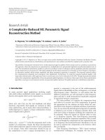
From Figures 7–12 this situation can be observed clearly.
For example, in Figure 7, which shows the average recon-
struction error for component 1, with the proposed method
using first scenario (APA1) the final reconstruction error
level is reached by around 3 million multiplications. A similar
level is reached with more than 20 million multiplications by

PO method. The multiplication required for the same level
for second scenario (APA2) is around 6 millions. On the
other hand using EM a better error level is obtained. Similar
results can be observed for component 2 as given in Figure 8.
From Figures 11 and 12 we see that again for Ex2 and Ex3 at
SNR 8 dB the proposed method reaches final reconstruction
error faster than PO method.
0
0.5
1
1.5
2

2.5
MSE
8101214
16
18 20
SNR (dB)
Ex1 component 1
APA1
APA2
PO
EM
CRB

Figure 3: Experimental MSE versus SNR for Ex1 component 1.
0
0.2
0.4
0.6
0.8
1
1.2
1.4
1.6
MSE
8101214

16
18 20
SNR (dB)
Ex1 component 2
APA1
APA2
PO
EM
CRB
Figure 4: Experimental MSE versus SNR for Ex1 component 2.
0
0.2

0.4
0.6
0.8
1
1.2
1.4
MSE
8101214
16
18 20
SNR (dB)
Ex2 component 1

APA1
APA2
PO
EM
CRB
Figure 5: Experimental MSE versus SNR for Ex2 component 1.
AscanbeseenfromFigures9 and 10 Increasing SNR to
14 or 20 dB for Ex1 makes the benefit of using APA1 or APA2
apparent. The same advantage was observed for Ex2 and Ex3
also. While at low SNR EM is usually better than the others
as the SNR increases, the advantage of EM is vanishing.
12 EURASIP Journal on Advances in Signal Processing

0
0.2
0.4
0.6
0.8
1
1.2
1.4
MSE
8101214
16
18 20

SNR (dB)
Ex3 component 2
APA1
APA2
EM
PO
CRB
Figure 6: Experimental MSE versus SNR for Ex3 component 2.
0
1
2
3

4
5
6
7
8
MSE
0 5 10 15 20 25 30 35 40
×10
6
Number of multiplications
Ex1 component 1 SNR 8 dB
APA1

APA2
PO
EM
CRB
Figure 7: Experimental MSE versus computation cost for Ex1 at
8dB(component1).
1
1.1
1.2
1.3
1.4
1.5

1.6
1.7
1.8
1.9
2
MSE
0 5 10 15 20 25 30 35 40
×10
6
Number of multiplications
Ex1 component 2 SNR 8 dB
APA1

APA2
PO
EM
CRB
Figure 8: Experimental MSE versus computation cost for Ex1 at
8dB(component2).
0
1
2
3
4
5

6
7
MSE
0 5 10 15 20 25 30 35
×10
6
Number of multiplications
Ex1 component 1 SNR 14 dB
APA1
APA2
PO
EM

CRB
Figure 9: Experimental MSE versus computation cost for Ex1 at
14 dB (component 1).
0
1
2
3
4
5
6
7
MSE

0 5 10 15 20 25 30
×10
6
Number of multiplications
Ex1 component 1 SNR 20 dB
APA1
APA2
PO
EM
CRB
Figure 10: Experimental MSE versus computation cost for Ex1 at
20 dB (component 1).

0
1
2
3
4
5
6
7
8
9
MSE
0 5 10 15 20 25

×10
6
Number of multiplications
Ex2 component 1 SNR 8 dB
APA1
APA2
PO
EM
CRB
Figure 11: Experimental MSE versus computation cost for Ex2 at
8dB(component1).
EURASIP Journal on Advances in Signal Processing 13

0
1
2
3
4
5
6
7
8
MSE
0 5 10 15 20 25 30 35
40

45
×10
6
Number of multiplications
Ex3 component 2 SNR 8 dB
APA1
APA2
PO
EM
CRB
Figure 12: Experimental MSE versus computation cost for Ex3 at
8dB(component2).

Looking at all the selected examples for all SNR values
it is clear that the proposed APA method has a superior
performance in terms of computations required to reach a
reconstruction error. APA1 which keeps alternating cycles
and phase iterations lower than APA2 is superior at high
SNR.
7. Conclusion
An iterative method has been proposed to estimate the
components of a multicomponent signal via parametric
ML estimation. The components on the TF plane are
assumed to be well separated. Though can be estimated,
it was also assumed that the number of components and

polynomial orders for amplitude and phase functions are
known. The resultant minimization problem was divided
into separate amplitude and phase minimizations. With the
proposed alternating phase and amplitude minimizations,
the computation cost of original minimization problem
reduced significantly. Also via simulations it was shown that,
at low SNR, a better reconstruction error is achieved when
the proposed method is used in an EM algorithm.
The initial estimates were obtained from time-frequency
distribution. They can also be obtained via PPT. Depending
on the performance of method by which initial estimates are
obtained, good initial conditions can be obtained, and the

computations can be saved even further.
References
[1] L. Cohen, “What is a multicomponent signal,” in Proceedings
of the International Conference on Acoustics, Speech, and Signal
Processing, vol. 5, pp. 113–116, 1992.
[2] H.M.Ozaktas¸, Z. Zalevsky, and M. A. Kutay, The Fractional
Fourier Transform with Applications in Optics and Signal
Processing, John Wiley & Sons, New York, NY, USA, 2000.
[3] L. B. Almeida, “Fractional fourier transform and time-
frequency representations,” IEEE Transactions on Signal Pro-
cessing, vol. 42, no. 11, pp. 3084–3091, 1994.
[4] H. M. Ozaktas, B. Barshan, D. Mendlovic, and L. Onural,

“Convolution, filtering, and multiplexing in fractional Fourier
domains and their relation to chirp and wavelet transforms,”
Journal of the Optical Society of America A,vol.11,no.2,pp.
547–559, 1994.
[5] G. F. Boudreaux-Bartels and T. W. Parks, “Time-varying
filtering and signal estimation using Wigner distribution
synthesis techniques,” IEEE Transactions on Acoustics, Speech,
and Signal Processing, vol. 34, no. 3, pp. 442–451, 1986.
[6] T.A.C.M.ClaasenandW.F.G.Mecklenbraiiker,“TheWigner
distribution-A tool for time-frequency signal analysis; Part
111: relations with other time-frequency signal transforma-
tions,” Philips Journal of Research, vol. 35, no. 6, pp. 372–389,

1980.
[7] W. Krattenthaler and F. Hlawatsch, “Time-frequency design
and processing of signals via smoothed Wigner distributions,”
IEEE Transactions on Signal Processing, vol. 41, no. 1, pp. 278–
287, 1993.
[8] G. C. Gaunaum and H. C. Strifors, “Signal analysis by means
of time-frequency (Wigner-Type) distributions—applications
to sonar and radar echoes,” Proceedings of the IEEE, vol. 84, no.
9, pp. 1231–1248, 1996.
[9] K. B. Yu and S. Cheng, “Signal synthesis from Pseudo-Wigner
distribution and applications,” IEEE Transactions on Acoustics,
Speech, and Signal Processing, vol. 35, no. 9, pp. 1289–1302,

1987.
[10] L. Cohen, “Time-frequency distributions—a review,” Proceed-
ings of the IEEE, vol. 77, no. 7, pp. 941–981, 1989.
[11] D. L. Jones and R. G. Baraniuk, “Adaptive optimal-kernel
time-frequency representation,” IEEE Transactions on Signal
Processing, vol. 43, no. 10, pp. 2361–2371, 1995.
[12] L. Cohen and T. E. Posch, “Positive time-frequency functions,”
IEEE Transactions on Acoustics, Speech, and Signal Processing,
vol. 33, no. 1, pp. 31–38, 1985.
[13] P. J. Loughlin, J. W. Pitton, and L. E. Atlas, “Construction of
positive time-frequency distributions,” IEEE Transactions on
Signal Processing, vol. 42, no. 10, pp. 2697–2705, 1994.

[14] B. Friedlander, “Parametric signal analysis using the poly-
nomial phase transform,” in Proceedings of the IEEE Signal
Processing Workshop Higher Order Statistics, Stanford Sierra
Camp, South Lake Tahoe, Calif, USA, June 1993.
[15] B. Friedlander and J. M. Francos, “Estimation of amplitude
and phase parameters of multicomponent signals,” IEEE
Transactions on Signal Processing, vol. 43, no. 4, pp. 917–926,
1995.
[16] S. Peleg, Estimation and detection with the discrete polynomial
transform, Ph.D. dissertation, Department of Electrical and
Computer Engineering, University of California, Davis, Calif,
USA, 1993.

[17] D. S. Pham and A. M. Zoubir, “Analysis of multicomponent
polynomial phase signals,” IEEE Transactions on Signal Process-
ing, vol. 55, no. 1, pp. 56–65, 2007.
[18] A. Francos and M. Porat, “Analysis and synthesis of multicom-
ponent signals using positive time-frequency distributions,”
IEEE Transactions on Signal Processing, vol. 47, no. 2, pp. 493–
504, 1999.
[19] D. B. Luenberger and Y. Ye, Linear and Nonlinear Optimiza-
tion, Springer, New York, NY, USA, 3rd edition, 2008.
[20] A. P. Dempster, N. M. Laird, and D. B. Rubin, “Maximum
likelihood from in-complete data via the em algorithm,”
Journal of the Royal Statistical Society

, vol. 39, no. 1, pp. 1–38,
1977.
14 EURASIP Journal on Advances in Signal Processing
[21] G. McLachlan and T. Krishnan, The EM Algorithm and
Extensions, John Wiley & Sons, New York, NY, USA, 1996.
[22] S. Zacks, The Theory of Statistical Inference,JohnWiley&Sons,
New York, NY, USA, 1971.
[23] C. R. Rao, Linear Statistical Inference and Its Applications,John
Wiley & Sons, New York, NY, USA, 1965.
[24] J. Nocedal and S. J. Wright, Numerical Optimization, Springer,
New York, NY, USA, 1999.