Advanced Microwave and Millimeter Wave Technologies Devices, Circuits and Systems Part 11 ppt

AdvancedMicrowaveandMillimeterWave
Technologies:SemiconductorDevices,CircuitsandSystems392
Among the items, the slope is set the top priority. Maintaining the slope, the return and
insertion losses are considered.
Firstly, let us start the design by changing the order of the basic circuit from 1 to 2.
(a) (b)
(c) (d)
Fig. 4. The 1st and 2nd order linear equalizers (a) 1st order circuit (b) Performance(1st
order) (c) 2nd order circuit (d) Performance(2nd order)

The reactive elements are found by having their resonance at the cut-off frequency given in
the specs. The resistors are computed, assumed that the T-networks are symmetric, to secure
the gradient of the amplitude curve parallel to the given slope. Increasing the order of the
equalizer, the slope performance has improved from Fig. 4(b) to Fig. 4(d). Taking into
account the fabrication based upon the microstrip line, the reactive elements are replaced by
the lossy transmission line(better for considering dispersion). The order of the entire circuit
should be increased and the final design lends the performance in the insertion and return
loss as follows.
Going through the tuning and trimming on the fabricated equalizer, the measured return
and insertion losses amount to less than -10 dB and roughly 9 dB throughout the
band(2GHz ~ 18GHz), respectively. Actually, the slightly non-linear behavior happens in
the vicinity of 18GHz and it is believed to stem from the design ignorant of the capacitance
parasitic to the resistors and transmission lines.
(a) (b)
(c)
Fig. 5. The 14th order linear equalizers (a) Insertion loss (b) Return loss (c) Photo of the
fabricated circuit

4. Conclusion

In this article, the design of a gain equalizer has been conceptualized to achieve the linear
slope over the very wide band 2GH ~ 18GHz and good return loss performance. Besides, it
has been implemented by fabrication with the microstrip transmission lines and SMT
resistors. The measured data prove the realized equalizer outputs the acceptable linearity in
the slope and return and insertion losses.

5. References

[1] Miodrag V. Gmitrovic et al, “Fixed and Variable Slope CATV Amplitude Equalizers,”
Applied Microwave & Wireless, Jan/Feb 1998, pp. 77-83.
[2] M. Sankara Narayana, “Gain Equalizer Flattens Attenuation Over 6-18 GHz,” Applied
Microwave & Wireless, November/December 1998.
[3] D.J.Mellor , “On the Design of Matched Equalizer of prescribed Gain Versus Frequency
Profile”. IEEE MTT-S International Microwave Symposium Digest , 1997, pp.308-
311.
[4] Broadband MIC Equalizers TWTA Output Response . IEEE Design Feature. Oct 1993
[5] S. Kahng et al, “Expanding the bandwidth of the linear gain equalizer: Ku-band
communication,” KEES Journal, Vol. KEESJ18, No. 2, pp. 105-110,Feb. 2007.
[6] H. Ishida, and K. Araki, “Design and Analysis of UWB Bandpass Filter with Ring Filter,”
in IEEE MTT-S Intl. Dig. June 2004 pp. 1307-1310.
Developingthe150%-FBWKu-BandLinearEqualizer 393
Among the items, the slope is set the top priority. Maintaining the slope, the return and
insertion losses are considered.
Firstly, let us start the design by changing the order of the basic circuit from 1 to 2.
(a) (b)
(c) (d)
Fig. 4. The 1st and 2nd order linear equalizers (a) 1st order circuit (b) Performance(1st
order) (c) 2nd order circuit (d) Performance(2nd order)

The reactive elements are found by having their resonance at the cut-off frequency given in

the specs. The resistors are computed, assumed that the T-networks are symmetric, to secure
the gradient of the amplitude curve parallel to the given slope. Increasing the order of the
equalizer, the slope performance has improved from Fig. 4(b) to Fig. 4(d). Taking into
account the fabrication based upon the microstrip line, the reactive elements are replaced by
the lossy transmission line(better for considering dispersion). The order of the entire circuit
should be increased and the final design lends the performance in the insertion and return
loss as follows.
Going through the tuning and trimming on the fabricated equalizer, the measured return
and insertion losses amount to less than -10 dB and roughly 9 dB throughout the
band(2GHz ~ 18GHz), respectively. Actually, the slightly non-linear behavior happens in
the vicinity of 18GHz and it is believed to stem from the design ignorant of the capacitance
parasitic to the resistors and transmission lines.
(a) (b)
(c)
Fig. 5. The 14th order linear equalizers (a) Insertion loss (b) Return loss (c) Photo of the
fabricated circuit

4. Conclusion

In this article, the design of a gain equalizer has been conceptualized to achieve the linear
slope over the very wide band 2GH ~ 18GHz and good return loss performance. Besides, it
has been implemented by fabrication with the microstrip transmission lines and SMT
resistors. The measured data prove the realized equalizer outputs the acceptable linearity in
the slope and return and insertion losses.

5. References

[1] Miodrag V. Gmitrovic et al, “Fixed and Variable Slope CATV Amplitude Equalizers,”
Applied Microwave & Wireless, Jan/Feb 1998, pp. 77-83.
[2] M. Sankara Narayana, “Gain Equalizer Flattens Attenuation Over 6-18 GHz,” Applied

Microwave & Wireless, November/December 1998.
[3] D.J.Mellor , “On the Design of Matched Equalizer of prescribed Gain Versus Frequency
Profile”. IEEE MTT-S International Microwave Symposium Digest , 1997, pp.308-
311.
[4] Broadband MIC Equalizers TWTA Output Response . IEEE Design Feature. Oct 1993
[5] S. Kahng et al, “Expanding the bandwidth of the linear gain equalizer: Ku-band
communication,” KEES Journal, Vol. KEESJ18, No. 2, pp. 105-110,Feb. 2007.
[6] H. Ishida, and K. Araki, “Design and Analysis of UWB Bandpass Filter with Ring Filter,”
in IEEE MTT-S Intl. Dig. June 2004 pp. 1307-1310.
AdvancedMicrowaveandMillimeterWave
Technologies:SemiconductorDevices,CircuitsandSystems394
[7] H. Wang, L. Zhu and W. Menzel, “Ultra-Wideband Bandpass Filter with Hybrid
Microstrip/CPW Structure,” IEEE Microwave And Wireless Components Letters,
vol. 15, pp. 844-846, December 2005
[8] S. Sun, and L. Zhu, “Capacitive-Ended Interdigital Coupled Lines for UWB Bandpass
Filters with Improved Out-of-Band Performances,” IEEE Microwave And Wireless
Components Letters, vol. 16, pp. 440-442, August 2006.
[9] W. Menzel, M. S. R. Tito, and L. Zhu, “Low-Loss Ultra-Wideband(UWB) Filters Using
Suspended Stripline,” in Proc. Asia-Pacific Microw. Conf. , Dec. 2005, vol. 4,
pp.2148-2151
[10] C L. Hsu, F C. Hsu, and J T. Kuo, “Microstrip Bandpass Filters for Ultra-
Wideband(UWB) Wireless Communications,” in IEEE MTT-S Intl. Dig. , June 2005,
pp.675-678
[11] C. Caloz and T. Itoh, Electromagnetic Metamaterials : Transmission Line Theory and
Microwave Applications, WILEY-INTERSCIENCE, John-Wiley & Sons Inc.,
Hoboken, NJ 2006
[12] S. Kahng, and J. Ju, “Left-Handedness based Bandpass Filter Design for RFID UHF-
Band applications,” in Proc. KJMW 2007, Nov 2007, vol. 1, pp.165-168.
[13] J. Ju and S. Kahng, “Design of the Miniaturaized UHF Bandpass Filter with the Wide
Stopband using the Inductive-Coupling Inverters and Metamaterials,” in Proc.

Korea Electromagnetic Engineering Society Conference 2007, Nov. 2007, vol. 1,
pp.5-8
[14] K. C. Gupta, R. Garg, I. Bahl, and P. Bhartia, Microstrip Lines and Slotlines, Artech
House Inc., Norwood, MA 1996

UltrawidebandBandpassFilterusingCompositeRight-and
Left-HandednessLineMetamaterialUnit-Cell 395
Ultrawideband Bandpass Filter using Composite Right- and Left-
HandednessLineMetamaterialUnit-Cell
SungtekKahng
X

Ultrawideband Bandpass Filter using
Composite Right- and Left-Handedness Line
Metamaterial Unit-Cell

Sungtek Kahng

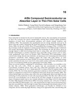
Abstract
The design of a new UWB bandpass filter is proposed, which is based upon the microstrip
Composite Right- and Left-Handed Transmission-line(CRLH-TL). In order to bring the
remarkable improvement in an attempt to reduce the size, taking the features of the
conventional periodic CRLH-TL, only one unit of the structure is chosen. So the component
less than a quarter-wavelength is realized to achieve the ultra wide band filtering without
the loss of the original advantage of the CRLH-TL. Guaranteeing the compactness in size,
the interdigitated coupled lines are used to realize the strong coupling for the design that
will be shown to have the size of ‘guided wavelength/9.4’, the fractional bandwidth over
100%, the insertion loss much less than 1 dB, and the flat group-delay with an acceptable
return loss performance in the predicted and measured results.

1. Introduction

In recent years, numerous studies have been conducted to exploit the benefits of the UWB
communication, since its unlicensed use was open to the public by the US FCC. As one of
many such research activities, the design methods of bandpass filters have been reported[6-
10].
Araki et al [6] designed the UWB bandpass filter whose bandwidth is formed by adding
zeros in the sections of the transmission line. The frequency response has notches at the
specific points as the very narrow regions for out-of-band suppression. H. Wang et al [7]
presented the microstrip-and-CPW bandpass filter for the UWB application, which is based
upon the Multi-Mode Resonator(MMR) in the form of multiples of quarter-wavelength, to
broaden the bandwidth and obtain the enlarged rejection region. The idea of the MMR of
the half wavelength is also used in [8] where the coupled lines of a quarter-wavelength are
used as the inverter. This work shows the extension of the lower and higher stopbands
owing to the increased coupling. A composite UWB filter was designed by W. Menzel et al
by combining lowpass and high pass filters as a suspended stripline structure with different
planes[9]. Independently, C. Hsu et al presented the composite microstrip filters for the
UWB application, where seven or eight TL sections of about quarter-wavelength are
sequentially connected[10]. Presently, we describe the design method of a new UWB filter
on the basis of the composite right- and left-handed transmission line(CRLH-TL)[11-13].
20
AdvancedMicrowaveandMillimeterWave
Technologies:SemiconductorDevices,CircuitsandSystems396
Different from the reference [11], we take just one segment(smaller than one quarter-
wavelength) from the periodic structure of the CRLH-TL to make the component very
compact. Besides, instead of mixing two types, for instance, hybrid of the microstrip and
CPW, the filter design is pursued with only the microstrip. Most of all, what features in our
present work is that the interdigital coupled lines much smaller than a quarter wavelength
and the grounded stub account for the strong capacitive coupling and the inductance for the
left-handedness, respectively, and the effective inductance of the interdigital capacitor and

the effective capacitance of the short-circuited inductor are used to decide the right-
handedness characteristics, in order to form a ultra wideband. And then going through the
implementation process, the predicted performances of the designed filter are given with
the measurement of the fabricated one to validate our design methodology, where the
design of the proposed BPF reveals the suitability for the UWB application, showing the size
reduction to the guided wavelength/9.4, the bandwidth more than 100%, the insertion loss
lower than 1 dB, the group-delay variation less than 0.5 ns with the good return loss
property.

2. Design of The Crlh-Tl Type Uwb Bpf

The left-handed medium as a metamaterial has been examined theoretically and
experimentally as it plays the lumped high pass filter circuit, and its unit cell in a periodic
transmission line is smaller than the guided wavelength. Instead of the pure left-
handedness, the CRLH-TL as a more practical circuit has been portrayed by C. Caloz et
al[11]. It is represented by Fig. 2-1.
Fig. 2-1. Equivalent circuit model of the conventional periodic CRLH -TL

There are three intermediate units of the periodic CRLH-TL and the i-th segment is marked
by the dotted line block in Fig. 1. The i-th segment consists of (C
Li
, L
Li
) for the left-
handedness and (C
Ri
, L
Ri
) for the right-handedness property. From the standpoint of the
purely left-handed unit, L

Ri
and C
Ri
can be considered parasitic inductance and capacitance
against C
Li
and L
Li
, respectively. However, in our design, we use the effective inductance L
Ri

and the effective capacitance C
Ri
for the purpose of forming a pass-band for the UWB filter.
As is addressed previously, only the basic unit, say, the i-th segment is taken for the present
work. Its symmetric version can be expressed a Pi-equivalent circuit in Fig. 2-2.
Fig. 2-2. Pi-equivalent circuit of the unit cell from the CRLH-TL

The ladder type of circuit in Fig. 1 has the exactly the same function as that in Fig. 2-2. But
the difference between them is the physical configuration, and this will be shed a light on
later. What is important in using the basic unit of the CRLH-TL in Fig. 2 is to determine the
values of the elements (C
Li
, L
Li
, C
Ri
, L
Ri
) that produce the performances appropriate to the

UWB BPF. We adopt the concept of the Balanced CRLH-TL in [11] to achieve a single broad
band without any gap in between the cut-off frequencies of highpass and lowpass filtering.
In the Balanced case, the three from four resonance phenomena lead to the following
relations.
LiLi
Li
CL
f

2
1

,
RiRi
Ri
CL
f

2
1

Oshisei
fff 
,
RiLiO
fff 
(2-1)
where
LiRi
sei

CL
f

2
1

,
RiLi
shi
CL
f

2
1


That f
sei
is let equal to f
shi
means the balance in the CRLH-TL, where f
Li
, f
Ri
, f
sei
, f
shi
, and f
O

correspond to the lower band-edge, upper band-edge, series resonance point, shunt
resonance point and center frequency, respectively. Solving the equations above, the circuit
elements are identified.
In order for a BPF to have the ultra wideband, a strong coupling is essential to the
implementation. In particular, the sufficient large amount of C
Li
is required.
Fig. 2-3. Microstrip interdigital coupled lines and grounded stub

As explained in the introduction with other design cases where the hybrid of the
microstrip/CPW or the cascaded transmissions of wavelengths are used, CLi should be
large enough, as the designers’ main concern. Like them, we need a strong capacitive
coupling, but proceed with the microstrip interdigital coupled lines. Even if the interdigital
UltrawidebandBandpassFilterusingCompositeRight-and
Left-HandednessLineMetamaterialUnit-Cell 397
Different from the reference [11], we take just one segment(smaller than one quarter-
wavelength) from the periodic structure of the CRLH-TL to make the component very
compact. Besides, instead of mixing two types, for instance, hybrid of the microstrip and
CPW, the filter design is pursued with only the microstrip. Most of all, what features in our
present work is that the interdigital coupled lines much smaller than a quarter wavelength
and the grounded stub account for the strong capacitive coupling and the inductance for the
left-handedness, respectively, and the effective inductance of the interdigital capacitor and
the effective capacitance of the short-circuited inductor are used to decide the right-
handedness characteristics, in order to form a ultra wideband. And then going through the
implementation process, the predicted performances of the designed filter are given with
the measurement of the fabricated one to validate our design methodology, where the
design of the proposed BPF reveals the suitability for the UWB application, showing the size
reduction to the guided wavelength/9.4, the bandwidth more than 100%, the insertion loss
lower than 1 dB, the group-delay variation less than 0.5 ns with the good return loss
property.

2. Design of The Crlh-Tl Type Uwb Bpf

The left-handed medium as a metamaterial has been examined theoretically and
experimentally as it plays the lumped high pass filter circuit, and its unit cell in a periodic
transmission line is smaller than the guided wavelength. Instead of the pure left-
handedness, the CRLH-TL as a more practical circuit has been portrayed by C. Caloz et
al[11]. It is represented by Fig. 2-1.
Fig. 2-1. Equivalent circuit model of the conventional periodic CRLH -TL

There are three intermediate units of the periodic CRLH-TL and the i-th segment is marked
by the dotted line block in Fig. 1. The i-th segment consists of (C
Li
, L
Li
) for the left-
handedness and (C
Ri
, L
Ri
) for the right-handedness property. From the standpoint of the
purely left-handed unit, L
Ri
and C
Ri
can be considered parasitic inductance and capacitance
against C
Li
and L
Li

, respectively. However, in our design, we use the effective inductance L
Ri

and the effective capacitance C
Ri
for the purpose of forming a pass-band for the UWB filter.
As is addressed previously, only the basic unit, say, the i-th segment is taken for the present
work. Its symmetric version can be expressed a Pi-equivalent circuit in Fig. 2-2.
Fig. 2-2. Pi-equivalent circuit of the unit cell from the CRLH-TL

The ladder type of circuit in Fig. 1 has the exactly the same function as that in Fig. 2-2. But
the difference between them is the physical configuration, and this will be shed a light on
later. What is important in using the basic unit of the CRLH-TL in Fig. 2 is to determine the
values of the elements (C
Li
, L
Li
, C
Ri
, L
Ri
) that produce the performances appropriate to the
UWB BPF. We adopt the concept of the Balanced CRLH-TL in [11] to achieve a single broad
band without any gap in between the cut-off frequencies of highpass and lowpass filtering.
In the Balanced case, the three from four resonance phenomena lead to the following
relations.
LiLi
Li
CL
f


2
1

,
RiRi
Ri
CL
f

2
1

Oshisei
fff 
,
RiLiO
fff 
(2-1)
where
LiRi
sei
CL
f

2
1

,
RiLi

shi
CL
f

2
1


That f
sei
is let equal to f
shi
means the balance in the CRLH-TL, where f
Li
, f
Ri
, f
sei
, f
shi
, and f
O
correspond to the lower band-edge, upper band-edge, series resonance point, shunt
resonance point and center frequency, respectively. Solving the equations above, the circuit
elements are identified.
In order for a BPF to have the ultra wideband, a strong coupling is essential to the
implementation. In particular, the sufficient large amount of C
Li
is required.
Fig. 2-3. Microstrip interdigital coupled lines and grounded stub

As explained in the introduction with other design cases where the hybrid of the
microstrip/CPW or the cascaded transmissions of wavelengths are used, CLi should be
large enough, as the designers’ main concern. Like them, we need a strong capacitive
coupling, but proceed with the microstrip interdigital coupled lines. Even if the interdigital
AdvancedMicrowaveandMillimeterWave
Technologies:SemiconductorDevices,CircuitsandSystems398
line has been around for quite some time, as is stated before, its geometric parameters will
be explored to find the desired effective inductance LRi as well as CLi in our design,
different from others. Fig. 2-3 presents the typical interdigital line. The geometry of an nIDF
fingered interdigital line described with W, l and S denoting the finger width, the finger
length and the spacing between the two adjacent fingers, respectively. The capacitance of
Fig. 2-3 is given as follows.
)1(
)('
)(
18
10
)(
3


IDF
re
n
kK
kK
pFC



(2-2)
where







b
a
k
4
tan
2

,
2
W
a 
,
2
SW
b



K(·) and K’(·) are the complete elliptic integral of the 1st kind and its complement. Along
with the series interdigital line, the grounded shunt stub plays an important role. The
expression as follows is commonly used for the inductance of the grounded stub and each

finger in the interdigital line(L
Ri
). Though it is an approximate formula, it helps us quickly
approach the initial size.

g
K
l
tW
t
W
l
lnHL 





]224.0193.1)[ln(102)(
4
(2-3)
where
)ln(145.057.0
h
W
K
g

h and t above mean the thickness of the substrate and metallization in use. The expressions
for the other circuit elements are found in [9] and used to correct the electrical behaviors

based upon Eqns (2) and (3). With all these values, physical sizes are iteratively exploited
until the acquisition of the desired performance.

3. Results of Implementation

Use First of all, the interdigital line’s size is calculated to realize the capacitance of 0.477pF
and its effective inductance of 5.53nH. Via the iterative steps using Eq’s (2) and (3), the
initial values are found W=0.20 mm, l =1.30mm, S=0.12 and n
IDF
=14.

(a)
(b)
(c)
(d)
Fig. 2-4. Interdigital line’s capacitance and inductance V.S. geometric changes (a) Number of
fingers V.S. Cs (b) Number of fingers VS. Cp (c) Number of fingers V.S. Ls (d) Length of the
finger V.S. Cp

This is followed by finding the physical dimensions of the grounded transmission line stub
whose W and l are 0.5 mm and 5.0 mm with 1.13nH and 0.20pF. For the substrate, FR4(ε
r
=
4.4 ) is used. And the circuit values result in the following dispersion diagram. Resorting to
the conventional periodic CRLH-TL concept, just for convenience, we check the critical
points, say, transmission and stop bands .

UltrawidebandBandpassFilterusingCompositeRight-and
Left-HandednessLineMetamaterialUnit-Cell 399
line has been around for quite some time, as is stated before, its geometric parameters will

be explored to find the desired effective inductance LRi as well as CLi in our design,
different from others. Fig. 2-3 presents the typical interdigital line. The geometry of an nIDF
fingered interdigital line described with W, l and S denoting the finger width, the finger
length and the spacing between the two adjacent fingers, respectively. The capacitance of
Fig. 2-3 is given as follows.
)1(
)('
)(
18
10
)(
3


IDF
re
n
kK
kK
pFC


(2-2)
where








b
a
k
4
tan
2

,
2
W
a 
,
2
SW
b



K(·) and K’(·) are the complete elliptic integral of the 1st kind and its complement. Along
with the series interdigital line, the grounded shunt stub plays an important role. The
expression as follows is commonly used for the inductance of the grounded stub and each
finger in the interdigital line(L
Ri
). Though it is an approximate formula, it helps us quickly
approach the initial size.

g
K
l

tW
t
W
l
lnHL 





]224.0193.1)[ln(102)(
4
(2-3)
where
)ln(145.057.0
h
W
K
g

h and t above mean the thickness of the substrate and metallization in use. The expressions
for the other circuit elements are found in [9] and used to correct the electrical behaviors
based upon Eqns (2) and (3). With all these values, physical sizes are iteratively exploited
until the acquisition of the desired performance.

3. Results of Implementation

Use First of all, the interdigital line’s size is calculated to realize the capacitance of 0.477pF
and its effective inductance of 5.53nH. Via the iterative steps using Eq’s (2) and (3), the
initial values are found W=0.20 mm, l =1.30mm, S=0.12 and n

IDF
=14.

(a)
(b)
(c)
(d)
Fig. 2-4. Interdigital line’s capacitance and inductance V.S. geometric changes (a) Number of
fingers V.S. Cs (b) Number of fingers VS. Cp (c) Number of fingers V.S. Ls (d) Length of the
finger V.S. Cp

This is followed by finding the physical dimensions of the grounded transmission line stub
whose W and l are 0.5 mm and 5.0 mm with 1.13nH and 0.20pF. For the substrate, FR4(ε
r
=
4.4 ) is used. And the circuit values result in the following dispersion diagram. Resorting to
the conventional periodic CRLH-TL concept, just for convenience, we check the critical
points, say, transmission and stop bands .

AdvancedMicrowaveandMillimeterWave
Technologies:SemiconductorDevices,CircuitsandSystems400
Fig. 2-5. Dispersion curve of the proposed UWB BPF

The refined physical dimensions based upon the initial values for the filter’s geometry, the
3D EM full-wave simulation has been carried out.

(a)













(b)
Fig. 2-6. S
11
and S
21
of the proposed UWB BPF (a) Simulation (b) measurement.

Frequency[GHz]

2 4 6 8 10 12 14
Scattering parameters[dB]
-60
-50
-40
-30
-20
-10
0
S
11
(Simulated)
S
21
(Simulated)
Frequency[GHz]
2 4 6 8 10 12 14
Scattering parameters[dB]
-60
-50
-40
-30
-20
-10
0
S
11
(Measured)
S
21

(Measured)
Fig. 2-6 plots the simulated scattering parameters S
11
and S
21
verified by the measurement.
Excellent agreement is shown between the simulated and measured S
21
with almost the
same transmission zeros, bandwidth over 100 % and insertion loss less than 1dB. Also, good
return loss is given despite the small discrepancy guessed due to the mechanical tolerance
error. Next, we need to check out the group-delay of the designed filter.
Fig.2- 7. Group-delay of the proposed UWB BPF : Simulation and measurement.

The variation of the group-delay is as small as less than 0.25 nsec over the passband. Lastly,
we show the photograph of our fabricated UWB BPF.

Fig. 2-8. Picture of the designed UWB BPF

The interdigital line sandwiched by the grounded stubs composes the proposed filter which
is about 4.7 mm long(far less than a quarter guided-wavelength).

4. Conclusion
The A new compact UWB BPF is proposed using the concept of the CRLH-TL. Only 1 unit
of the CRLH-TL is taken for enhanced size reduction and implemented with the interdigital
line and grounded stubs with their effective parasitics for the UWB. The designed BPF
performs with the BW over 100%, good insertion and return loss, and flat group-delay with
the overall size to the guided wavelength/9.4.

M easur ed
2 3 4 5 6 7 8 9 10 111 12
-1. 0
-0. 5
0. 0
0. 5
1. 0
-1. 5
1. 5
Fr equency[ GH z]
GroupDelay[nsec]
Simulated
UltrawidebandBandpassFilterusingCompositeRight-and
Left-HandednessLineMetamaterialUnit-Cell 401
Fig. 2-5. Dispersion curve of the proposed UWB BPF

The refined physical dimensions based upon the initial values for the filter’s geometry, the
3D EM full-wave simulation has been carried out.

(a)













(b)
Fig. 2-6. S
11
and S
21
of the proposed UWB BPF (a) Simulation (b) measurement.

Frequency[GHz]
2 4 6 8 10 12 14
Scattering parameters[dB]
-60
-50
-40
-30
-20

-10
0
S
11
(Simulated)
S
21
(Simulated)
Frequency[GHz]
2 4 6 8 10 12 14
Scattering parameters[dB]
-60
-50
-40
-30
-20
-10
0
S
11
(Measured)
S
21
(Measured)
Fig. 2-6 plots the simulated scattering parameters S
11
and S
21
verified by the measurement.
Excellent agreement is shown between the simulated and measured S

21
with almost the
same transmission zeros, bandwidth over 100 % and insertion loss less than 1dB. Also, good
return loss is given despite the small discrepancy guessed due to the mechanical tolerance
error. Next, we need to check out the group-delay of the designed filter.
Fig.2- 7. Group-delay of the proposed UWB BPF : Simulation and measurement.

The variation of the group-delay is as small as less than 0.25 nsec over the passband. Lastly,
we show the photograph of our fabricated UWB BPF.

Fig. 2-8. Picture of the designed UWB BPF

The interdigital line sandwiched by the grounded stubs composes the proposed filter which
is about 4.7 mm long(far less than a quarter guided-wavelength).

4. Conclusion
The A new compact UWB BPF is proposed using the concept of the CRLH-TL. Only 1 unit
of the CRLH-TL is taken for enhanced size reduction and implemented with the interdigital
line and grounded stubs with their effective parasitics for the UWB. The designed BPF
performs with the BW over 100%, good insertion and return loss, and flat group-delay with
the overall size to the guided wavelength/9.4.


M easur ed
2 3 4 5 6 7 8 9 10 111 12
-1. 0
-0. 5
0. 0
0. 5
1. 0

-1. 5
1. 5
Fr equency[ GH z]
GroupDelay[nsec]
Simulated
AdvancedMicrowaveandMillimeterWave
Technologies:SemiconductorDevices,CircuitsandSystems402
5. Acknowledgment

This work was supported by the IT R&D program of MKE/IITA. [2009-S-001-01, Study of
technologies for improving the RF spectrum characteristics by using the meta-
electromagnetic structure]

6. References

[1] Miodrag V. Gmitrovic et al, “Fixed and Variable Slope CATV Amplitude Equalizers,”
Applied Microwave & Wireless, Jan/Feb 1998, pp. 77-83.
[2] M. Sankara Narayana, “Gain Equalizer Flattens Attenuation Over 6-18 GHz,” Applied
Microwave & Wireless, November/December 1998.
[3] D.J.Mellor , “On the Design of Matched Equalizer of prescribed Gain Versus Frequency
Profile”. IEEE MTT-S International Microwave Symposium Digest , 1997, pp.308-
311.
[4] Broadband MIC Equalizers TWTA Output Response . IEEE Design Feature. Oct 1993
[5] S. Kahng et al, “Expanding the bandwidth of the linear gain equalizer: Ku-band
communication,” KEES Journal, Vol. KEESJ18, No. 2, pp. 105-110,Feb. 2007.
[6] H. Ishida, and K. Araki, “Design and Analysis of UWB Bandpass Filter with Ring Filter,”
in IEEE MTT-S Intl. Dig. June 2004 pp. 1307-1310.
[7] H. Wang, L. Zhu and W. Menzel, “Ultra-Wideband Bandpass Filter with Hybrid
Microstrip/CPW Structure,” IEEE Microwave And Wireless Components Letters,
vol. 15, pp. 844-846, December 2005

[8] S. Sun, and L. Zhu, “Capacitive-Ended Interdigital Coupled Lines for UWB Bandpass
Filters with Improved Out-of-Band Performances,” IEEE Microwave And Wireless
Components Letters, vol. 16, pp. 440-442, August 2006.
[9] W. Menzel, M. S. R. Tito, and L. Zhu, “Low-Loss Ultra-Wideband(UWB) Filters Using
Suspended Stripline,” in Proc. Asia-Pacific Microw. Conf. , Dec. 2005, vol. 4,
pp.2148-2151
[10] C L. Hsu, F C. Hsu, and J T. Kuo, “Microstrip Bandpass Filters for Ultra-
Wideband(UWB) Wireless Communications,” in IEEE MTT-S Intl. Dig. , June 2005,
pp.675-678
[11] C. Caloz and T. Itoh, Electromagnetic Metamaterials : Transmission Line Theory and
Microwave Applications, WILEY-INTERSCIENCE, John-Wiley & Sons Inc.,
Hoboken, NJ 2006
[12] S. Kahng, and J. Ju, “Left-Handedness based Bandpass Filter Design for RFID UHF-
Band applications,” in Proc. KJMW 2007, Nov 2007, vol. 1, pp.165-168.
[13] J. Ju and S. Kahng, “Design of the Miniaturaized UHF Bandpass Filter with the Wide
Stopband using the Inductive-Coupling Inverters and Metamaterials,” in Proc.
Korea Electromagnetic Engineering Society Conference 2007, Nov. 2007, vol. 1,
pp.5-8
[14] K. C. Gupta, R. Garg, I. Bahl, and P. Bhartia, Microstrip Lines and Slotlines, Artech
House Inc., Norwood, MA 1996

ExtendedSourceSizeCorrectionFactorinAntennaGainMeasurements 403
ExtendedSourceSizeCorrectionFactorinAntennaGainMeasurements
AlekseySoloveyandRajMittra
x

Extended Source Size Correction Factor in
Antenna Gain Measurements

Aleksey Solovey and Raj Mittra

L-3 Communications ESSCO, Pennsylvania State University
USA

1. Introduction

In this chapter we consider the extended source size correction factor that is widely utilized
in antenna gain measurements when extraterrestrial extended radio sources are in use.
Extended radio sources having an angular size that is comparable or even larger than the
antenna’s far-field power pattern Half Power Beam Width (HPBW) are often used to
determine various antenna parameters including gain of electrically large antenna apertures
(Baars, 1973). The use of such sources often becomes almost inevitable since the far-field
distance of electrically large antennas can reach tens or even hundreds kilometers, which
makes it impractical if not impossible to employ the conventional far-field antenna
transmitter-receiver test range technique.
To illustrate the importance of the problem let’s consider 30m radio astronomy antenna at
10GHz and 96GHz frequency bands. Its far-field zone distances are 60km and 580km with
the HPBW equal to 4’ and 0.42’ respectively. For the comparison, among the strongest
cosmic radio sources, Cassiopeia A has 4’ and Sygnus A has 0.7’ of their disk angular sizes
(Guidici & Castelli, 1971). Even for the 7m communication antenna working at 20 GHz, the
far-field distance is 6.5km and the far-field patterns HPBW is 1.4º, while the angular size of
the Sun or the Moon disks are about of 0.5º (Guidici & Castelli, 1971).
When the radio source angular size is comparable with the antenna HPBW, the antenna
radiation pattern is averaged within the solid spatial angle subtended to the source.
Therefore, the measured antenna gain value appears to be less than what would be expected
for the antenna’s effective collecting area and the aperture illumination and the resulting
gain measurements must be corrected by the extended source size correction factor to
account for the convolution of the extended radio source angular size, angular source
brightness distribution and the shape of the antenna’s far-field radiation pattern. In this
chapter two kinds of extended radio sources, having either uniform or Gaussian brightness
distributions over the source disk (Baars, 1973; Kraus, 1986), along with three kinds of the

most usable “Polynomial-on-Pedestal,” Gaussian, and Taylor antenna aperture
illuminations are examined for circular and rectangular antenna apertures.
As a result of the above considerations and based on the literature survey, the complete set
of simple analytical expressions that accurately approximate the value of the extended
source size correction factor have been derived and/or developed for circular and
21
AdvancedMicrowaveandMillimeterWave
Technologies:SemiconductorDevices,CircuitsandSystems404

rectangular antenna apertures and for all the above combinations of extended radio source
brightness distributions and antenna aperture illuminations. Those expressions eliminate
the need to perform complicated and often impractical numerical integrations in order to
evaluate the extended source size correction factor value for the case of particular
measurement. The approximate analytical expressions for the extended source size
correction factor for rectangular antenna apertures along with their tolerances for circular
and rectangular apertures are obtained for the first time in literature.
Because the extended source size correction factor most conveniently can be expressed
through the ratio between the extended source angular size (or its HPBW) and the antenna’s
far-field radiation pattern HPBW, the approximations of the antenna’s HPBW for all three
types of antenna aperture illuminations and for circular and rectangular antenna apertures
are considered as a supplementary problem. As a result, numerous simple and accurate
analytical expressions for the antenna’s far-field pattern HPBW for circular and rectangular
antenna apertures and for all three types of antenna aperture illuminations have been
developed. This also eliminates the need to perform complicated and often impractical
numerical integrations in order to evaluate the antenna’s far-field pattern HPBW value for
the particular antenna size(s) and aperture illumination(s). In addition, for circular and
rectangular antenna apertures these expressions are shown in the form of plots.
While in this chapter, we consider the extended source size correction factor from the
prospective of the antenna gain measurement, it should be noted that the same factor can
also be utilized for the solution of the inverse problem: the measurement of the unknown

temperature and/or flux density of a randomly polarized extended radio source using the
electrically large antenna with a known antenna far-field power pattern (Ko, 1961).

2. Extended Cosmic Radio Sources and Extended Source Size Correction
Factor in Antenna Gain Measurements


The IEEE Standard Std 149-1979 for the antenna test procedures (Kummer at al., 1979)
defines the extended source size correction factor K by the following expression:








S
S
dF
s
B
dB
K
n
s
)()(
)(
(1)

where B
s
(

) is the angular brightness distribution of the extended radio source, F
n
(

) is the
normalized pencil beam antenna far-field power pattern, such that at the antenna boresight
(direction of the peak of the main beam) F
n
(0) = 1, and

S
is the solid angle subtended to the
extended radio source. To obtain the correct antenna gain, the gain value measured using
the extended radio source should be multiplied by K.
In order to understand the meaning and the applicability of definition (1) let’s first establish
the relations between the power pattern F
n
(

) and the antenna far-field radiation power
pattern F(

) that is normalized the way that the total power transmitted or received by the
antenna within the entire 4π steradian solid angle equals to one power unit:

1)()(
44






dFAdF
n
(2)

where A is a constant multiplier that needs to be found. In case of the omnidirectional
antenna when F
n
(

) = 1 at any direction of the solid angle

, condition (2) gives the
following value of that multiplier A
omni
:



4
1
1

4



omniomni
AdA (3)

By definition (Balanis, 2005), the maximum antenna gain G
max
is the ratio of the maximum
antenna radiation intensity, i. e. A, to the radiation intensity averaged over all directions, i. e.
A
omni
:



4
4
max
omni
max
G
AA
A
A
G 
(4)

Based on (2) and (4) one can notice that the denominator in (1) is proportional to the power

P
extended source
received by the antenna whose maximum gain value is G
max
in the case when its
far-field pattern HPBW is comparable or greater than the size of the extended radio source
spatial angle:




S
dF
G
BP
n
max
sourceextended s
)(
4
)(

(5)

The numerator in (1) is proportional to the power P
point source
received by the same antenna in
the case when its far-field antenna pattern HPBW is much bigger than the angular size of
extended radio source and thus, the value F
n

(Ω) in (5) can be substituted by 1 within the
source spatial angle:



S
d
G
BP
max
ssourcepoint

4
)(
(6)

The relations (5) and (6) can be used by both ways: to find the unknown maximum antenna
gain and the radiation pattern based on the measured power received by the antenna and
the known source brightness distribution or, conversely, to find the unknown source
brightness distribution based on the measured power received by the antenna and the
known maximum antenna gain and the radiation pattern. Either way, the ratio between the
received power (6) and the received power (5) is equal to the extended source size correction
factor defined by (1) and represents the correction that should be made if the extended radio
source, but not the point source, is used in the measurement procedure.
In order to compute the extended source size correction factor using its definition (1), both
the extended source brightness B
s
(

) and the normalized antenna power pattern F

n
(

) as a
function of the solid angle subtended to the extended source should be known. In following
sections we review expressions for the extended source correction factor already existed in
literature, discuss and specify the considered set of functions B
s
(

) and F
n
(

), its relations
with actual extended radio sources and antenna configurations and disclose numerous
ExtendedSourceSizeCorrectionFactorinAntennaGainMeasurements 405

rectangular antenna apertures and for all the above combinations of extended radio source
brightness distributions and antenna aperture illuminations. Those expressions eliminate
the need to perform complicated and often impractical numerical integrations in order to
evaluate the extended source size correction factor value for the case of particular
measurement. The approximate analytical expressions for the extended source size
correction factor for rectangular antenna apertures along with their tolerances for circular
and rectangular apertures are obtained for the first time in literature.
Because the extended source size correction factor most conveniently can be expressed
through the ratio between the extended source angular size (or its HPBW) and the antenna’s
far-field radiation pattern HPBW, the approximations of the antenna’s HPBW for all three
types of antenna aperture illuminations and for circular and rectangular antenna apertures
are considered as a supplementary problem. As a result, numerous simple and accurate

analytical expressions for the antenna’s far-field pattern HPBW for circular and rectangular
antenna apertures and for all three types of antenna aperture illuminations have been
developed. This also eliminates the need to perform complicated and often impractical
numerical integrations in order to evaluate the antenna’s far-field pattern HPBW value for
the particular antenna size(s) and aperture illumination(s). In addition, for circular and
rectangular antenna apertures these expressions are shown in the form of plots.
While in this chapter, we consider the extended source size correction factor from the
prospective of the antenna gain measurement, it should be noted that the same factor can
also be utilized for the solution of the inverse problem: the measurement of the unknown
temperature and/or flux density of a randomly polarized extended radio source using the
electrically large antenna with a known antenna far-field power pattern (Ko, 1961).

2. Extended Cosmic Radio Sources and Extended Source Size Correction
Factor in Antenna Gain Measurements


The IEEE Standard Std 149-1979 for the antenna test procedures (Kummer at al., 1979)
defines the extended source size correction factor K by the following expression:








S
S
dF
s

B
dB
K
n
s
)()(
)(
(1)

where B
s
(

) is the angular brightness distribution of the extended radio source, F
n
(

) is the
normalized pencil beam antenna far-field power pattern, such that at the antenna boresight
(direction of the peak of the main beam) F
n
(0) = 1, and

S
is the solid angle subtended to the
extended radio source. To obtain the correct antenna gain, the gain value measured using
the extended radio source should be multiplied by K.
In order to understand the meaning and the applicability of definition (1) let’s first establish
the relations between the power pattern F
n

(

) and the antenna far-field radiation power
pattern F(

) that is normalized the way that the total power transmitted or received by the
antenna within the entire 4π steradian solid angle equals to one power unit:



1)()(
44






dFAdF
n
(2)

where A is a constant multiplier that needs to be found. In case of the omnidirectional
antenna when F
n
(

) = 1 at any direction of the solid angle

, condition (2) gives the

following value of that multiplier A
omni
:



4
1
1
4



omniomni
AdA (3)

By definition (Balanis, 2005), the maximum antenna gain G
max
is the ratio of the maximum
antenna radiation intensity, i. e. A, to the radiation intensity averaged over all directions, i. e.
A
omni
:



4
4
max
omni

max
G
AA
A
A
G 
(4)

Based on (2) and (4) one can notice that the denominator in (1) is proportional to the power
P
extended source
received by the antenna whose maximum gain value is G
max
in the case when its
far-field pattern HPBW is comparable or greater than the size of the extended radio source
spatial angle:




S
dF
G
BP
n
max
sourceextended s
)(
4
)(


(5)

The numerator in (1) is proportional to the power P
point source
received by the same antenna in
the case when its far-field antenna pattern HPBW is much bigger than the angular size of
extended radio source and thus, the value F
n
(Ω) in (5) can be substituted by 1 within the
source spatial angle:



S
d
G
BP
max
ssourcepoint

4
)(
(6)

The relations (5) and (6) can be used by both ways: to find the unknown maximum antenna
gain and the radiation pattern based on the measured power received by the antenna and
the known source brightness distribution or, conversely, to find the unknown source
brightness distribution based on the measured power received by the antenna and the
known maximum antenna gain and the radiation pattern. Either way, the ratio between the

received power (6) and the received power (5) is equal to the extended source size correction
factor defined by (1) and represents the correction that should be made if the extended radio
source, but not the point source, is used in the measurement procedure.
In order to compute the extended source size correction factor using its definition (1), both
the extended source brightness B
s
(

) and the normalized antenna power pattern F
n
(

) as a
function of the solid angle subtended to the extended source should be known. In following
sections we review expressions for the extended source correction factor already existed in
literature, discuss and specify the considered set of functions B
s
(

) and F
n
(

), its relations
with actual extended radio sources and antenna configurations and disclose numerous
AdvancedMicrowaveandMillimeterWave
Technologies:SemiconductorDevices,CircuitsandSystems406

novel simple analytical expressions that accurately approximate the value of extended
source size correction factor for those combinations of B

s
(

) and F
n
(

).

3. Existing Approximate Analytical Formulae for Extended Source Size
Correction Factor


Based on definition (1) of the extended source size correction factor and making various
simplifying assumptions about the source brightness distribution B
s
(

) and the normalized
antenna far-field power pattern F
n
(

), several approximate analytical expressions for the
extended source correction factor have been developed in literature.
For the case of a Gaussian source brightness distribution and a Gaussian antenna far-field
power pattern (Guidici & Castelli, 1971) and (Baars, 1973) stated the following expression
for the extended source correction factor K:
2
1 sK  (7)

where s is the ratio of the extended source HPBW to the antenna HPBW. For the case of a
uniform source brightness distribution and a Gaussian antenna far-field power pattern (Ko,
1961) expresses value of K as:
])2ln(exp[1
)2ln(
2
2
s
s
K


(8)

where s is the ratio of the disk source angular diameter to the antenna HPBW. For the case
of a uniform source brightness distribution and an antenna far-field power pattern that
corresponds with a uniform antenna aperture illumination (Ko, 1961) expresses the value of
K as:
)]616.1()616.1(1[4
)616.1(
2
0
2
1
2
sJsJ
s
K



(9)

where s is the ratio of the source disk diameter to the antenna HPBW.
It should be noted that expressions (7) – (9) were derived under the assumption of a small
value of variable s, i. e., when the extended source angular size is noticeably less than the
antenna pattern HPBW and only for the circular antenna aperture.
In Figure 1, the approximate values of the extended source size correction factor as a
function of the ratio of the source diameter or the source HPBW to the antenna HPBW and
given by expressions (7) – (9) are shown in comparison. As is seen from Figure 1, the values
given by expressions (8) and (9) are very close to each other, while being significantly
different from values given by the expression (7). Expressions (7) – (9) were selected among
few others because they represent the best approximations of the extended source size
correction factor available in the literature for both uniform and Gaussian extended source
brightness distributions that are used the most in antenna measurements and/or
calibrations.
However, there are also several problems that are associated with these approximations.
First, approximations (7) and (8) are based on the shape of the antenna far-field power

pattern rather than based on the shape of the antenna aperture illumination and its edge
illumination taper, which are actually known in practice. Secondly, in order to use
expressions (7) – (9), the antenna HPBW as a function of the type of the aperture
illumination and its edge illumination taper has to be known. Third, not all combinations of
aperture illuminations and extended source brightness distributions used in practice are
covered by (7) – (9). Fourth, all expressions (7) – (9) were derived for the small value of the
source size to antenna HPBW ratio and it’s accuracy for the case when this ratio isn’t small is
unknown. Fifth, these expressions were derived only for circular antenna apertures and do
not cover rectangular apertures that become increasingly popular for the modern solid state
antennas. Sixth, expressions (7) – (9) do not explicitly depend on the antenna aperture edge
illumination taper, which is manifestly wrong since the normalized antenna power pattern

F
n
(Ω) and therefore, the extended source size correction factor do depend on it.
Further in this chapter we will amend and expand expressions (7) – (9) the way that
eliminates all its deficiencies that were mentioned above.

0 0 . 2 0. 4 0 .6 0 . 8 1 1 . 2 1 . 4
S o u r c e S i z e o v e r A n t e n n a B e a m w i d t h
0
1
2
3
4
5
E x t e n d e d So u r c e S i z e C o r r e c ti o n F a c t o r , d B


0 1 2 3 4 5
S o u r c e S i z e ov e r A n t e n n a Be a m w i d t h
0
2
4
6
8
1 0
1 2
1 4
E x t e n d e d S o u r c e S i z e C o r r e c t i o n F a c t o r , d B

Fig. 1. Approximate expressions for extended source size correction factor in comparison.

Plot legend: solid red – expression (9); long-dashed blue – expression (7); and short-dashed
green – expression (8);

ExtendedSourceSizeCorrectionFactorinAntennaGainMeasurements 407

novel simple analytical expressions that accurately approximate the value of extended
source size correction factor for those combinations of B
s
(

) and F
n
(

).

3. Existing Approximate Analytical Formulae for Extended Source Size
Correction Factor


Based on definition (1) of the extended source size correction factor and making various
simplifying assumptions about the source brightness distribution B
s
(

) and the normalized
antenna far-field power pattern F
n
(


), several approximate analytical expressions for the
extended source correction factor have been developed in literature.
For the case of a Gaussian source brightness distribution and a Gaussian antenna far-field
power pattern (Guidici & Castelli, 1971) and (Baars, 1973) stated the following expression
for the extended source correction factor K:
2
1 sK  (7)

where s is the ratio of the extended source HPBW to the antenna HPBW. For the case of a
uniform source brightness distribution and a Gaussian antenna far-field power pattern (Ko,
1961) expresses value of K as:
])2ln(exp[1
)2ln(
2
2
s
s
K


(8)

where s is the ratio of the disk source angular diameter to the antenna HPBW. For the case
of a uniform source brightness distribution and an antenna far-field power pattern that
corresponds with a uniform antenna aperture illumination (Ko, 1961) expresses the value of
K as:
)]616.1()616.1(1[4
)616.1(
2
0

2
1
2
sJsJ
s
K


(9)

where s is the ratio of the source disk diameter to the antenna HPBW.
It should be noted that expressions (7) – (9) were derived under the assumption of a small
value of variable s, i. e., when the extended source angular size is noticeably less than the
antenna pattern HPBW and only for the circular antenna aperture.
In Figure 1, the approximate values of the extended source size correction factor as a
function of the ratio of the source diameter or the source HPBW to the antenna HPBW and
given by expressions (7) – (9) are shown in comparison. As is seen from Figure 1, the values
given by expressions (8) and (9) are very close to each other, while being significantly
different from values given by the expression (7). Expressions (7) – (9) were selected among
few others because they represent the best approximations of the extended source size
correction factor available in the literature for both uniform and Gaussian extended source
brightness distributions that are used the most in antenna measurements and/or
calibrations.
However, there are also several problems that are associated with these approximations.
First, approximations (7) and (8) are based on the shape of the antenna far-field power

pattern rather than based on the shape of the antenna aperture illumination and its edge
illumination taper, which are actually known in practice. Secondly, in order to use
expressions (7) – (9), the antenna HPBW as a function of the type of the aperture
illumination and its edge illumination taper has to be known. Third, not all combinations of

aperture illuminations and extended source brightness distributions used in practice are
covered by (7) – (9). Fourth, all expressions (7) – (9) were derived for the small value of the
source size to antenna HPBW ratio and it’s accuracy for the case when this ratio isn’t small is
unknown. Fifth, these expressions were derived only for circular antenna apertures and do
not cover rectangular apertures that become increasingly popular for the modern solid state
antennas. Sixth, expressions (7) – (9) do not explicitly depend on the antenna aperture edge
illumination taper, which is manifestly wrong since the normalized antenna power pattern
F
n
(Ω) and therefore, the extended source size correction factor do depend on it.
Further in this chapter we will amend and expand expressions (7) – (9) the way that
eliminates all its deficiencies that were mentioned above.

0 0 . 2 0. 4 0 .6 0 . 8 1 1 . 2 1 . 4
S o u r c e S i z e o v e r A n t e n n a B e a m w i d t h
0
1
2
3
4
5
E x t e n d e d So u r c e S i z e C o r r e c ti o n F a c t o r , d B


0 1 2 3 4 5
S o u r c e S i z e ov e r A n t e n n a Be a m w i d t h
0
2
4
6

8
1 0
1 2
1 4
E x t e n d e d S o u r c e S i z e C o r r e c t i o n F a c t o r , d B

Fig. 1. Approximate expressions for extended source size correction factor in comparison.
Plot legend: solid red – expression (9); long-dashed blue – expression (7); and short-dashed
green – expression (8);

AdvancedMicrowaveandMillimeterWave
Technologies:SemiconductorDevices,CircuitsandSystems408

4. Brightness Distributions of Extended Cosmic Radio Sources Used in
Antenna Gain Measurements

The detailed description of most cosmic extended radio sources that are used in the
electrically large antenna measurements and calibrations along with the discussion of
various aspects of such measurements is given, for example, in (Baars, 1973), (Guidici &
Castelli, 1971) and (Kraus, 1986).
From the extended source correction factor evaluation standpoint it’s enough to notice that
most of these extended radio sources have circular disk shape with either axially
symmetrical Gaussian or uniform brightness distributions over the solid angle that is
subtended to the extended radio source disk (Baars, 1973), (Kraus, 1986). Those sources are
almost entirely incoherent and that is why in (1) the antenna far-field power pattern, as
oppose to the antenna far-field radiation field pattern, is in use. For example, the Cassiopeia
A has a uniform brightness distribution, while the Orion A has an axially symmetrical
Gaussian brightness distribution over a source disk (Baars, 1973).
Thus, for the purpose of this chapter, we will consider only these two, the uniform and the
Gaussian extended radio source brightness distributions, which can be written in following

forms:
2/,0
2/,1
),(
{
s
s
B
uniS






(10)



















2
2
2lnexp),(
s
B
GaussS



(11)

where θ
s
is the angular size of the extended radio source. In the case of the uniform source
brightness distribution θ
s
is the physical angular size of the source disk. In the case of the
Gaussian source brightness distribution, the source angular size θ
s
is defined as a source
HPBW, i. e., the angular size at which the brightness of the source is half of its maximum at
the center of the source disk.
It should be stressed that the assumed properties of the extended radio source namely, the
radiation incoherence and the types of source brightness distribution (10) and (11), are
essential for the correct simulation of the extended source size correction factor.

5. Illumination Functions and Antenna Patterns for Circular and Rectangular
Antenna Apertures

5.1 Circular Antenna Aperture Case
In order to calculate the value of the extended source size correction factor (1) except of the
extended source brightness distribution function B
s
(

) that was described in previous
section, the antenna far-field power pattern F
n
(

) needs to be known. Unlike the extended
source brightness distribution B
s
(

) the antenna far-field power pattern F
n
(

) for almost all
practical cases is not an analytically defined function and is rather defined through the
particular illumination of the antenna aperture.

For the purpose of this chapter we chose the three most usable circularly symmetrical
aperture illumination functions: “Polynomial-on-Pedestal,” Gaussian, and Taylor. For
convenience, we use following forms of these aperture illumination functions for the

circular aperture:
2
2
2
1)1(

















d
r
BBf
ApPoly
(12)









2
)
2
ln(exp
d
r
B
ApGauss
f (13)

][
)
2
(1(
0
2
0


jJ
d
r
jJ
f
ApTaylor









(14)

where r is the value of the radius vector from the center of the circular aperture, d is the
diameter of the antenna aperture, B is the aperture edge illumination taper (0 ≤ B ≤ 1), and
the constant β in the expression (14) can be found from the equation:

B
jJ
1
][
0


(15)

The aperture edge illumination taper is usually expressed in dB, thus for convenience, we
introduce the constant c that is associated with constant B by:

Bc
10
log20 (16)

Here’s another useful constant that is associated with constant B and will be extensively
used throughout the chapter:

Bb


1 (17)

The example of all three circular aperture illumination functions (12) – (14) are shown in
Figure 2 for comparison. As is seen from plots in Figure 2, expression (12) – (14) are
normalized so that all aperture illuminations (12) – (14) have the same maximum value of 1
at the center of the aperture and the same minimum value at the edge of the aperture that is
equal to the value of the aperture edge illumination taper B.
Knowing the antenna aperture illuminations (12) – (14) and using the aperture approach for
the antenna pattern calculation, the normalized antenna power pattern for the circular
antenna aperture can be expressed, according to (Johnson at all, 1993) as follows:

ExtendedSourceSizeCorrectionFactorinAntennaGainMeasurements 409

4. Brightness Distributions of Extended Cosmic Radio Sources Used in
Antenna Gain Measurements

The detailed description of most cosmic extended radio sources that are used in the
electrically large antenna measurements and calibrations along with the discussion of
various aspects of such measurements is given, for example, in (Baars, 1973), (Guidici &
Castelli, 1971) and (Kraus, 1986).
From the extended source correction factor evaluation standpoint it’s enough to notice that
most of these extended radio sources have circular disk shape with either axially
symmetrical Gaussian or uniform brightness distributions over the solid angle that is
subtended to the extended radio source disk (Baars, 1973), (Kraus, 1986). Those sources are

almost entirely incoherent and that is why in (1) the antenna far-field power pattern, as
oppose to the antenna far-field radiation field pattern, is in use. For example, the Cassiopeia
A has a uniform brightness distribution, while the Orion A has an axially symmetrical
Gaussian brightness distribution over a source disk (Baars, 1973).
Thus, for the purpose of this chapter, we will consider only these two, the uniform and the
Gaussian extended radio source brightness distributions, which can be written in following
forms:
2/,0
2/,1
),(
{
s
s
B
uniS






(10)



















2
2
2lnexp),(
s
B
GaussS



(11)

where θ
s
is the angular size of the extended radio source. In the case of the uniform source
brightness distribution θ
s
is the physical angular size of the source disk. In the case of the
Gaussian source brightness distribution, the source angular size θ
s
is defined as a source

HPBW, i. e., the angular size at which the brightness of the source is half of its maximum at
the center of the source disk.
It should be stressed that the assumed properties of the extended radio source namely, the
radiation incoherence and the types of source brightness distribution (10) and (11), are
essential for the correct simulation of the extended source size correction factor.

5. Illumination Functions and Antenna Patterns for Circular and Rectangular
Antenna Apertures

5.1 Circular Antenna Aperture Case
In order to calculate the value of the extended source size correction factor (1) except of the
extended source brightness distribution function B
s
(

) that was described in previous
section, the antenna far-field power pattern F
n
(

) needs to be known. Unlike the extended
source brightness distribution B
s
(

) the antenna far-field power pattern F
n
(

) for almost all

practical cases is not an analytically defined function and is rather defined through the
particular illumination of the antenna aperture.

For the purpose of this chapter we chose the three most usable circularly symmetrical
aperture illumination functions: “Polynomial-on-Pedestal,” Gaussian, and Taylor. For
convenience, we use following forms of these aperture illumination functions for the
circular aperture:
2
2
2
1)1(

















d
r

BBf
ApPoly
(12)








2
)
2
ln(exp
d
r
B
ApGauss
f (13)

][
)
2
(1(
0
2
0



jJ
d
r
jJ
f
ApTaylor








(14)

where r is the value of the radius vector from the center of the circular aperture, d is the
diameter of the antenna aperture, B is the aperture edge illumination taper (0 ≤ B ≤ 1), and
the constant β in the expression (14) can be found from the equation:

B
jJ
1
][
0


(15)

The aperture edge illumination taper is usually expressed in dB, thus for convenience, we

introduce the constant c that is associated with constant B by:

Bc
10
log20 (16)

Here’s another useful constant that is associated with constant B and will be extensively
used throughout the chapter:

Bb 1 (17)

The example of all three circular aperture illumination functions (12) – (14) are shown in
Figure 2 for comparison. As is seen from plots in Figure 2, expression (12) – (14) are
normalized so that all aperture illuminations (12) – (14) have the same maximum value of 1
at the center of the aperture and the same minimum value at the edge of the aperture that is
equal to the value of the aperture edge illumination taper B.
Knowing the antenna aperture illuminations (12) – (14) and using the aperture approach for
the antenna pattern calculation, the normalized antenna power pattern for the circular
antenna aperture can be expressed, according to (Johnson at all, 1993) as follows:

AdvancedMicrowaveandMillimeterWave
Technologies:SemiconductorDevices,CircuitsandSystems410

0 1 0 2 0 3 0 4 0 5 0 6 0
R a d i u s , i n c h e s
- 1 0
- 8
- 6
- 4
- 2

0
A p e r t u r e D i s t r i b u t i o n , d B


0 1 0 2 0 3 0 4 0 5 0 6 0
R a d i u s , i n c h e s
- 3 0
- 2 5
- 2 0
- 1 5
- 1 0
- 5
0
A p e r t u r e D i s t r i b u t i o n , d B

Fig. 2. Comparison between “Polynomial-on-Pedestal” (solid red), Gaussian (long-dashed
blue) and Taylor (short-dashed green) aperture illuminations for 10dB (upper) and 30dB
(lower) circular aperture edge illumination taper.

2
5.0
0
5.0
0
0
),(
)sin(),(
)(


















d
i
d
i
drBrf
drkrJBrf
F
ni


(18)

where k = 2π/λ is the wavenumber, θ is the antenna pattern off-boresight angle, and the
index i stands for any of aperture illumination functions (12) – (14). For instance, i = 1
corresponds with the expression (12), i = 2 corresponds with the expression (13) and i = 3

corresponds with the expression (14).
It should be noted that in spite of well known deficiencies of the aperture approach for the
antenna pattern calculation that approach is quite adequate for this particular application
since in (1) only values of function (18) in the vicinity of the antenna main lobe are actually
used. Plots in Figure 3 illustrate the difference between antenna patterns computed using
(18) for all three aperture illuminations (12) – (14).
As is seen from these plots the difference between antenna patterns for all three aperture
illuminations becomes noticeable well outside of the 3dB beamwidth off-boresight direction
even for heavily tapered aperture illuminations. It should be also noticed that when the
aperture edge illumination taper approaches 0dB, which means that the constant B

approaches 1, all three aperture illumination functions (12) – (14) approach the uniform
illumination and thus, their antenna patterns are also converged to each other.

0 0 . 5 1 1 . 5 2 2 . 5 3
B o r e d i g h t A n g l e , d e g r e e
- 8 0
- 6 0
- 4 0
- 2 0
0
A n t e n n a P a t t e r n , d B


0 0 . 5 1 1 . 5 2 2 . 5 3
B o r e s i g h t A n g l e , d e g r e e
- 8 0
- 6 0
- 4 0
- 2 0

0
A n t e n n a P a t t e r n , d B

Fig. 3. Comparison between antenna patterns for “Polynomial-on-Pedestal” (solid red),
Gaussian (long-dashed blue), and Taylor (short-dashed green) aperture illumination
functions with 10dB (upper) and 30dB (bottom) circular aperture edge illumination taper.

5.2 Rectangular Antenna Aperture Case
It was assumed that for the case of the rectangular aperture the same aperture illumination
functions (12) – (14) are applied in combination along each of the Cartesian coordinate x and
y in a form of its direct product:

),(),(),,,(
yjxiyxij
ByfBxfByBxf 
(19)

where i and j stand for any of aperture illuminations (12) – (14). For example, the
rectangular aperture illumination that is the “Polynomial-on-Pedestal” along the X-axis and
is the Gaussian one along the Y-axis is described by the following expression:

ExtendedSourceSizeCorrectionFactorinAntennaGainMeasurements 411

0 1 0 2 0 3 0 4 0 5 0 6 0
R a d i u s , i n c h e s
- 1 0
- 8
- 6
- 4
- 2

0
A p e r t u r e D i s t r i b u t i o n , d B


0 1 0 2 0 3 0 4 0 5 0 6 0
R a d i u s , i n c h e s
- 3 0
- 2 5
- 2 0
- 1 5
- 1 0
- 5
0
A p e r t u r e D i s t r i b u t i o n , d B

Fig. 2. Comparison between “Polynomial-on-Pedestal” (solid red), Gaussian (long-dashed
blue) and Taylor (short-dashed green) aperture illuminations for 10dB (upper) and 30dB
(lower) circular aperture edge illumination taper.

2
5.0
0
5.0
0
0
),(
)sin(),(
)(


















d
i
d
i
drBrf
drkrJBrf
F
ni


(18)

where k = 2π/λ is the wavenumber, θ is the antenna pattern off-boresight angle, and the
index i stands for any of aperture illumination functions (12) – (14). For instance, i = 1
corresponds with the expression (12), i = 2 corresponds with the expression (13) and i = 3

corresponds with the expression (14).
It should be noted that in spite of well known deficiencies of the aperture approach for the
antenna pattern calculation that approach is quite adequate for this particular application
since in (1) only values of function (18) in the vicinity of the antenna main lobe are actually
used. Plots in Figure 3 illustrate the difference between antenna patterns computed using
(18) for all three aperture illuminations (12) – (14).
As is seen from these plots the difference between antenna patterns for all three aperture
illuminations becomes noticeable well outside of the 3dB beamwidth off-boresight direction
even for heavily tapered aperture illuminations. It should be also noticed that when the
aperture edge illumination taper approaches 0dB, which means that the constant B

approaches 1, all three aperture illumination functions (12) – (14) approach the uniform
illumination and thus, their antenna patterns are also converged to each other.

0 0 . 5 1 1 . 5 2 2 . 5 3
B o r e d i g h t A n g l e , d e g r e e
- 8 0
- 6 0
- 4 0
- 2 0
0
A n t e n n a P a t t e r n , d B


0 0 . 5 1 1 . 5 2 2 . 5 3
B o r e s i g h t A n g l e , d e g r e e
- 8 0
- 6 0
- 4 0
- 2 0

0
A n t e n n a P a t t e r n , d B

Fig. 3. Comparison between antenna patterns for “Polynomial-on-Pedestal” (solid red),
Gaussian (long-dashed blue), and Taylor (short-dashed green) aperture illumination
functions with 10dB (upper) and 30dB (bottom) circular aperture edge illumination taper.

5.2 Rectangular Antenna Aperture Case
It was assumed that for the case of the rectangular aperture the same aperture illumination
functions (12) – (14) are applied in combination along each of the Cartesian coordinate x and
y in a form of its direct product:

),(),(),,,(
yjxiyxij
ByfBxfByBxf 
(19)

where i and j stand for any of aperture illuminations (12) – (14). For example, the
rectangular aperture illumination that is the “Polynomial-on-Pedestal” along the X-axis and
is the Gaussian one along the Y-axis is described by the following expression:

AdvancedMicrowaveandMillimeterWave
Technologies:SemiconductorDevices,CircuitsandSystems412






























22
2
2112
)
2
ln(exp]
2
1)[1(

),(),(),,,(
y
y
x
xx
yxyx
d
y
B
d
x
BB
ByfBxfByBxf
(20)

where d
x
and d
y
are the rectangular aperture width and height, x and y are coordinates in the
aperture plane with the origin in the center of the aperture, and B
x
and B
y
are aperture edge
illumination tapers that, in general, have different values along X and Y axes.
Based on the rectangular aperture illumination function (19) and using the same aperture
approach that was used for the case of the circular aperture, the normalized antenna power
pattern for the rectangular aperture can be written, according to (Johnson, R. C. at all, 1993)
as follows:

2
0 0
0 0
5.0
5.0
5.0
5.0
),,,(
)]sincos(sinexp[),,,(
),(














 
 


x

d
y
d
x
d
y
d
dxdyByBxf
dxdyyxkByBxf
F
yxij
yxij
nij


(21)

where the integration can be done just across the quarter of the aperture because all
integrand functions are even in respect to variables x and y. Because all integrand functions
are also separable in respect to variables x and y, the expression (21) can be simplified even
further and present the antenna pattern of the rectangular aperture as a product of two
terms one of which contains integrals only along the x coordinate axis and the other contains
integrals only along the y coordinate axis:

2
0
0
0
0
5.0

5.0
5.0
5.0
),(
]sinsinexp[),(
),(
]cossinexp[),(
),(





















y

d
y
d
x
d
x
d
dyByf
dykyByf
dxBxf
dxkxBxf
F
yj
yj
xi
xi
nij


(22)

The expression (22) is valid for the rectangular aperture antenna pattern with separable
aperture illuminations along x and y axes and means, for instance, that the antenna pattern
in principal plane at φ = 0° depends only on the illumination function f
i
(x,B
x
), while in the
other principal plane at φ = 90°, it depends only on the illumination function f
j

(y,B
y
).Plots in
Figure 4 illustrate the difference between antenna patterns in principal planes computed
using (22) for all three aperture illuminations (12) – (14). These plots were calculated for the
rectangular aperture with the same area as the area of the circular aperture that was used to
calculate plots in Figure 3. As is seen from these plots, similarly to the circular aperture case
differences in antenna patterns for all three aperture illuminations (12) – (14) become

noticeable well outside of the 3dB beamwidth off-boresight angles even for heavily tapered
aperture illuminations. The comparison between antenna patterns for circular (Fig. 3) and
rectangular (Fig. 4) antennas shows just some quantitative but not qualitative differences
between them.

0 0 . 5 1 1 . 5 2 2 . 5 3
B o r e s i g h t A n g l e , d e g r e e
- 8 0
- 6 0
- 4 0
- 2 0
0
A n t e n n a P a t t e r n , d B


0 0 . 5 1 1 . 5 2 2 . 5 3
B o r e s i g h t A n g l e , d e g r e e
- 8 0
- 6 0
- 4 0
- 2 0

0
A n t e n n a P a t t e r n , d B

Fig. 4. Comparison between antenna patterns for “Polynomial-on-Pedestal” (solid red),
Gaussian (long-dashed blue), and Taylor (short-dashed green) aperture illuminations with
10dB (upper) and 30dB (bottom) rectangular aperture edge illumination taper.

6. Simple and Accurate Approximation of Antenna HPBW for Circular and
Rectangular Apertures

6.1 Circular Antenna Aperture Case
Based on the general definition of the extended source correction factor (1) and using
expressions (10), (11) for the source brightness distribution and expressions (18), (22) for the
circular and rectangular aperture antenna power pattern, it is possible now to calculate the
exact value for the extended source size correction factor. However, in order to compare the
exact value of the extended source size correction factor with its approximations given by
expressions (7) – (9), the value of the antenna pattern HPBW should be known with a high
ExtendedSourceSizeCorrectionFactorinAntennaGainMeasurements 413






























22
2
2112
)
2
ln(exp]
2
1)[1(
),(),(),,,(
y
y
x
xx

yxyx
d
y
B
d
x
BB
ByfBxfByBxf
(20)

where d
x
and d
y
are the rectangular aperture width and height, x and y are coordinates in the
aperture plane with the origin in the center of the aperture, and B
x
and B
y
are aperture edge
illumination tapers that, in general, have different values along X and Y axes.
Based on the rectangular aperture illumination function (19) and using the same aperture
approach that was used for the case of the circular aperture, the normalized antenna power
pattern for the rectangular aperture can be written, according to (Johnson, R. C. at all, 1993)
as follows:

2
0 0
0 0
5.0

5.0
5.0
5.0
),,,(
)]sincos(sinexp[),,,(
),(














 
 


x
d
y
d
x
d

y
d
dxdyByBxf
dxdyyxkByBxf
F
yxij
yxij
nij


(21)

where the integration can be done just across the quarter of the aperture because all
integrand functions are even in respect to variables x and y. Because all integrand functions
are also separable in respect to variables x and y, the expression (21) can be simplified even
further and present the antenna pattern of the rectangular aperture as a product of two
terms one of which contains integrals only along the x coordinate axis and the other contains
integrals only along the y coordinate axis:

2
0
0
0
0
5.0
5.0
5.0
5.0
),(
]sinsinexp[),(

),(
]cossinexp[),(
),(





















y
d
y
d
x
d

x
d
dyByf
dykyByf
dxBxf
dxkxBxf
F
yj
yj
xi
xi
nij


(22)

The expression (22) is valid for the rectangular aperture antenna pattern with separable
aperture illuminations along x and y axes and means, for instance, that the antenna pattern
in principal plane at φ = 0° depends only on the illumination function f
i
(x,B
x
), while in the
other principal plane at φ = 90°, it depends only on the illumination function f
j
(y,B
y
).Plots in
Figure 4 illustrate the difference between antenna patterns in principal planes computed
using (22) for all three aperture illuminations (12) – (14). These plots were calculated for the

rectangular aperture with the same area as the area of the circular aperture that was used to
calculate plots in Figure 3. As is seen from these plots, similarly to the circular aperture case
differences in antenna patterns for all three aperture illuminations (12) – (14) become

noticeable well outside of the 3dB beamwidth off-boresight angles even for heavily tapered
aperture illuminations. The comparison between antenna patterns for circular (Fig. 3) and
rectangular (Fig. 4) antennas shows just some quantitative but not qualitative differences
between them.

0 0 . 5 1 1 . 5 2 2 . 5 3
B o r e s i g h t A n g l e , d e g r e e
- 8 0
- 6 0
- 4 0
- 2 0
0
A n t e n n a P a t t e r n , d B


0 0 . 5 1 1 . 5 2 2 . 5 3
B o r e s i g h t A n g l e , d e g r e e
- 8 0
- 6 0
- 4 0
- 2 0
0
A n t e n n a P a t t e r n , d B

Fig. 4. Comparison between antenna patterns for “Polynomial-on-Pedestal” (solid red),
Gaussian (long-dashed blue), and Taylor (short-dashed green) aperture illuminations with

10dB (upper) and 30dB (bottom) rectangular aperture edge illumination taper.

6. Simple and Accurate Approximation of Antenna HPBW for Circular and
Rectangular Apertures

6.1 Circular Antenna Aperture Case
Based on the general definition of the extended source correction factor (1) and using
expressions (10), (11) for the source brightness distribution and expressions (18), (22) for the
circular and rectangular aperture antenna power pattern, it is possible now to calculate the
exact value for the extended source size correction factor. However, in order to compare the
exact value of the extended source size correction factor with its approximations given by
expressions (7) – (9), the value of the antenna pattern HPBW should be known with a high
AdvancedMicrowaveandMillimeterWave
Technologies:SemiconductorDevices,CircuitsandSystems414

degree of accuracy for each aperture illuminations (12) – (14) for circular and rectangular
apertures. This is ultimately needed because the argument s of the extended source size
correction factor approximate expressions (7) – (9) is defined as:

HPBWantenna
HPBWsourceordiametersource
s 
(23)

According, for example, to (Johnson at all, 1993), the circular antenna HPBW can be
estimated through the simple formula:
d
HPBW



 (24)

where λ is a wavelength, d is the antenna diameter and the α is the beamwidth multiplier in
degrees that depends on the type of aperture illumination and edge illumination taper. The
rough estimation of α as a function of the aperture edge illumination taper, without taking
into account the type of the aperture illumination, was given in (Johnson at all, 1993):

c05238.19486.55 

(25)

where c is define in (16) as an absolute value of the edge illumination taper in dB. The
number of significant digits in (25) is misleading because the six digits computational
accuracy implied by the expression (25) can not be achieved based solely on the value of the
edge illumination taper, regardless of the type of the aperture illumination.
The numerical simulations of the circular antenna beamwidth using the expression (18) for
the circular antenna radiation pattern and for all three type of aperture illuminations (12) –
(14) give the values of the beamwidth multiplier α that are summarized in Table 1 and
illustrated in Figure 5.

6.2 Rectangular Antenna Aperture Case
As it was mentioned in section 5.2 for the rectangular antenna aperture illuminated by the
separable aperture illumination function (19), antenna pattern cuts in principal planes (along
the X or Y axes) are independent of each other and, as it follows from (22), depend
exclusively on its own aperture illumination function regardless of illumination function
that is applied along the opposite axis in the aperture plane. Thus, to calculate the
rectangular antenna HPBW in principal planes, one can still employ the expression (24)
substituting the circular aperture diameter d by the width d
x
or the height d

y
of the
rectangular aperture, respectively.
The numerical simulations of the rectangular antenna beamwidth using the expression (22)
for the rectangular antenna radiation pattern and for all three type of aperture illuminations
(12) – (14) give the values of the beamwidth multiplier α that are summarized in Table 2 and
illustrated in Figure 6.


0 5 1 0 1 5 2 0
E d g e Ta p er , d B
6 0
6 2 . 5
6 5
6 7 . 5
7 0
7 2 . 5
7 5
A p p ro x im at e 3 d B B e a mw i dt h M u l t ip ly e r , d eg r ee


0 1 0 2 0 3 0 4 0 5 0 6 0
E d g e T a p e r , d B
6 0
7 0
8 0
9 0
1 0 0
1 1 0
A p p r o xi m at e 3 d B B e am w id t h Mu l t ip l ie r , d e gr e e

Fig. 5. Approximate 3dB beamwidth multiplier α used in (24) as a function of aperture edge
illumination taper for circular aperture and “Polynomial-on-Pedestal” (solid red), Gaussian
(long-dashed blue) and Taylor (short-dashed green) aperture illuminations.

Antenna
Aperture
Illumination
Approximate Beamwidth Multiplier α in degrees
Circular Aperture, c ≤ 40dB

Max
Error,
%

Polynomial
58.862 + 0.53523c

+ 0.039795c
2

- 0.001575c
3

+ 0.00001562c
4

0.13
Gaussian
58.862 + 0.5865c

+ 0.01089c
2


- 0.000094c
3

0.055
Taylor
58.862 + 0.6247c

+ 0.0048c
2


- 0.000086c
3

0.095
Table 1. Approximate formulae for antenna pattern beamwidth multiplier α used in (24) for
circular aperture.
ExtendedSourceSizeCorrectionFactorinAntennaGainMeasurements 415

degree of accuracy for each aperture illuminations (12) – (14) for circular and rectangular
apertures. This is ultimately needed because the argument s of the extended source size
correction factor approximate expressions (7) – (9) is defined as:

HPBWantenna
HPBWsourceordiametersource

s 
(23)

According, for example, to (Johnson at all, 1993), the circular antenna HPBW can be
estimated through the simple formula:
d
HPBW


 (24)

where λ is a wavelength, d is the antenna diameter and the α is the beamwidth multiplier in
degrees that depends on the type of aperture illumination and edge illumination taper. The
rough estimation of α as a function of the aperture edge illumination taper, without taking
into account the type of the aperture illumination, was given in (Johnson at all, 1993):

c05238.19486.55 

(25)

where c is define in (16) as an absolute value of the edge illumination taper in dB. The
number of significant digits in (25) is misleading because the six digits computational
accuracy implied by the expression (25) can not be achieved based solely on the value of the
edge illumination taper, regardless of the type of the aperture illumination.
The numerical simulations of the circular antenna beamwidth using the expression (18) for
the circular antenna radiation pattern and for all three type of aperture illuminations (12) –
(14) give the values of the beamwidth multiplier α that are summarized in Table 1 and
illustrated in Figure 5.

6.2 Rectangular Antenna Aperture Case

As it was mentioned in section 5.2 for the rectangular antenna aperture illuminated by the
separable aperture illumination function (19), antenna pattern cuts in principal planes (along
the X or Y axes) are independent of each other and, as it follows from (22), depend
exclusively on its own aperture illumination function regardless of illumination function
that is applied along the opposite axis in the aperture plane. Thus, to calculate the
rectangular antenna HPBW in principal planes, one can still employ the expression (24)
substituting the circular aperture diameter d by the width d
x
or the height d
y
of the
rectangular aperture, respectively.
The numerical simulations of the rectangular antenna beamwidth using the expression (22)
for the rectangular antenna radiation pattern and for all three type of aperture illuminations
(12) – (14) give the values of the beamwidth multiplier α that are summarized in Table 2 and
illustrated in Figure 6.


0 5 1 0 1 5 2 0
E d g e Ta p er , d B
6 0
6 2 . 5
6 5
6 7 . 5
7 0
7 2 . 5
7 5
A p p ro x im at e 3 d B B e a mw i dt h M u l t ip ly e r , d eg r ee

0 1 0 2 0 3 0 4 0 5 0 6 0
E d g e T a p e r , d B
6 0
7 0
8 0
9 0
1 0 0
1 1 0
A p p r o xi m at e 3 d B B e am w id t h Mu l t ip l ie r , d e gr e e

Fig. 5. Approximate 3dB beamwidth multiplier α used in (24) as a function of aperture edge
illumination taper for circular aperture and “Polynomial-on-Pedestal” (solid red), Gaussian
(long-dashed blue) and Taylor (short-dashed green) aperture illuminations.

Antenna
Aperture
Illumination
Approximate Beamwidth Multiplier α in degrees
Circular Aperture, c ≤ 40dB

Max
Error,
%

Polynomial
58.862 + 0.53523c

+ 0.039795c
2

- 0.001575c
3

+ 0.00001562c
4

0.13
Gaussian
58.862 + 0.5865c

+ 0.01089c
2


- 0.000094c
3

0.055
Taylor
58.862 + 0.6247c

+ 0.0048c
2


- 0.000086c
3

0.095
Table 1. Approximate formulae for antenna pattern beamwidth multiplier α used in (24) for

circular aperture.