Advanced Microwave and Millimeter Wave Technologies Devices, Circuits and Systems Part 14 pptx

AdvancedMicrowaveandMillimeterWave
Technologies:SemiconductorDevices,CircuitsandSystems512

The values of C are
DjqDpC
kkk
 , where p
k
and q
k
are chosen to minimize the PAPR
value, and the constant D is known both at the transmitter and the receiver. Fig. 19 presents
this solution for the case of a 16-QAM signal.
In Fig. 19, what we can see is that the black points could also be transmitted, but no new
information is added. This means that we can transmit the same digital symbol either using
the white points or the black points for the same base information bit, so the modulator have
some redundancy, which is chosen in order to minimize the PAPR.
The main problem is the increase in BER. Nevertheless, the augmented capability to reduce
PAPR is quite satisfactory.
Other possible available technique is the Tone Reservation (Tellado & Cioffi, 1998), where
the underneath idea is to reserve, that means, to select some sub carriers in order that the
overall RF signal has a reduced PAPR. In DSL communication systems this is normally done
in the low SNR tones, since they will not be very important for the overall signal
demodulation. So, in this case, we will add some information, C, to the unused tones to
reduce the overall PAPR in the time domain scenario. The unused tones are called the
reserved tones and normally do not carry data or they cannot carry data reliably due to their
low SNR. It is exactly these tones that are used to send optimum vector C that was selected
to reduce large peak power samples of OFDM symbols. The method is very simple to
implement, and the receiver could ignore the symbols carried on the unused tones, without
any complex demodulation process, neither extra tail bits.

Other simple but important technique is known as Amplitude Clipping plus Filtering
(Vaananen et al., 2002), which is obviously the one that can achieve improved results and is
less complex to apply. Nevertheless the clipping increases the occupied bandwidth and
simultaneously degrades significantly the in-band distortion, giving rise to the increase of
BER, due to its nonlinearity nature. The technique is based mainly on the following
procedure: if the signal is below a certain threshold, then we let the signal as is, at the
output, nevertheless if it passes that threshold then the signal should be clipped as is
presented in expression (8).

Ax
Ax
Ae
x
y
xj






,
)(

(8)

where
)(x

is the phase of the input signal x.

The main problem of this technique is that somehow we are distorting the signal generating
nonlinear distortion both in-band and out-of-band. The in-band distortion cannot be filtered
out, and some form of linearizer should be used or other form of reconstruction of the signal
prior to the reception block. The out-of-band emission, usually called spectral regrowth, can
be filtered out, but the filtering process will increase again the PAPR. For that reason, some
algorithms are used sequentially with clipping and filtering in order to converge to a
minimum value. This technique can be further associated with other schemes to improve the
PAPR overall solution.
Finally, we describe a scheme that is called Companding / Expanding technique (Jiang et
al., 2005), which is very similar to clipping, but the signal is not actually clipped, but rather
companded or expanded accordingly to its amplitude. This technique was used since the

analogue telephone lines were the voice was companded in order to reduce its dynamic
range problems encountered through the transmission over the copper lines. Most of the
authors have dedicated their time to select the optimum form of the companding function in
order to simultaneously reduce the PAPR and improve the BER performance. Fig. 20
presents one of these schemes implementation.


Fig. 20. Companding and Expanding implementation

One possibility for the companding function is the well-known μ-law, expression (9).



 
11,
1ln
1ln
)sgn()( 



 x
u
xu
xxF
(9)

The drawbacks of this solution are similar to the clipping technique, but in this case the
nonlinear distortion can be somehow post-distorted at the receiver more efficiently, since
the nonlinearity is not as severe as the clipping form.

4. Example Applications

In this section, we will present possible real-world applications of several of previous
described receiving architectures, in which we will describe some evaluated experiments.
These include configurations that are being used in emergent fields, such as RFID and SDR
systems. In these fields the multi-standard reception and the receiver PAPR minimization
techniques analyzed can bring attractive improvements.

4.1 Radio Frequency Identification Applications
An RFID system is basically composed of two main blocks: the TAG and the READER
(Fig. 21).

ReceiverFront-EndArchitectures–AnalysisandEvaluation 513

The values of C are
DjqDpC
kkk



, where p
k
and q
k
are chosen to minimize the PAPR
value, and the constant D is known both at the transmitter and the receiver. Fig. 19 presents
this solution for the case of a 16-QAM signal.
In Fig. 19, what we can see is that the black points could also be transmitted, but no new
information is added. This means that we can transmit the same digital symbol either using
the white points or the black points for the same base information bit, so the modulator have
some redundancy, which is chosen in order to minimize the PAPR.
The main problem is the increase in BER. Nevertheless, the augmented capability to reduce
PAPR is quite satisfactory.
Other possible available technique is the Tone Reservation (Tellado & Cioffi, 1998), where
the underneath idea is to reserve, that means, to select some sub carriers in order that the
overall RF signal has a reduced PAPR. In DSL communication systems this is normally done
in the low SNR tones, since they will not be very important for the overall signal
demodulation. So, in this case, we will add some information, C, to the unused tones to
reduce the overall PAPR in the time domain scenario. The unused tones are called the
reserved tones and normally do not carry data or they cannot carry data reliably due to their
low SNR. It is exactly these tones that are used to send optimum vector C that was selected
to reduce large peak power samples of OFDM symbols. The method is very simple to
implement, and the receiver could ignore the symbols carried on the unused tones, without
any complex demodulation process, neither extra tail bits.
Other simple but important technique is known as Amplitude Clipping plus Filtering
(Vaananen et al., 2002), which is obviously the one that can achieve improved results and is
less complex to apply. Nevertheless the clipping increases the occupied bandwidth and
simultaneously degrades significantly the in-band distortion, giving rise to the increase of
BER, due to its nonlinearity nature. The technique is based mainly on the following

procedure: if the signal is below a certain threshold, then we let the signal as is, at the
output, nevertheless if it passes that threshold then the signal should be clipped as is
presented in expression (8).

Ax
Ax
Ae
x
y
xj






,
)(

(8)

where
)(x

is the phase of the input signal x.
The main problem of this technique is that somehow we are distorting the signal generating
nonlinear distortion both in-band and out-of-band. The in-band distortion cannot be filtered
out, and some form of linearizer should be used or other form of reconstruction of the signal
prior to the reception block. The out-of-band emission, usually called spectral regrowth, can
be filtered out, but the filtering process will increase again the PAPR. For that reason, some

algorithms are used sequentially with clipping and filtering in order to converge to a
minimum value. This technique can be further associated with other schemes to improve the
PAPR overall solution.
Finally, we describe a scheme that is called Companding / Expanding technique (Jiang et
al., 2005), which is very similar to clipping, but the signal is not actually clipped, but rather
companded or expanded accordingly to its amplitude. This technique was used since the

analogue telephone lines were the voice was companded in order to reduce its dynamic
range problems encountered through the transmission over the copper lines. Most of the
authors have dedicated their time to select the optimum form of the companding function in
order to simultaneously reduce the PAPR and improve the BER performance. Fig. 20
presents one of these schemes implementation.


Fig. 20. Companding and Expanding implementation

One possibility for the companding function is the well-known μ-law, expression (9).



 
11,
1ln
1ln
)sgn()( 


 x
u
xu

xxF
(9)

The drawbacks of this solution are similar to the clipping technique, but in this case the
nonlinear distortion can be somehow post-distorted at the receiver more efficiently, since
the nonlinearity is not as severe as the clipping form.

4. Example Applications

In this section, we will present possible real-world applications of several of previous
described receiving architectures, in which we will describe some evaluated experiments.
These include configurations that are being used in emergent fields, such as RFID and SDR
systems. In these fields the multi-standard reception and the receiver PAPR minimization
techniques analyzed can bring attractive improvements.

4.1 Radio Frequency Identification Applications
An RFID system is basically composed of two main blocks: the TAG and the READER
(Fig. 21).

AdvancedMicrowaveandMillimeterWave
Technologies:SemiconductorDevices,CircuitsandSystems514


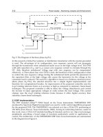
Fig. 21. RFID system

The Tag (or transponder) is a small device that serves as identifier of a person or an object in
which it was implemented. When asked by the reader, returns the information contained
within its small microchip. It should be noted, however, that despite this being the most
common method, there are active tags that transmit information without the presence of the
reader. The reader can be considered the "brain" of an RFID system. It is responsible for

liaison between external systems of data processing (computer-data based) and the tags, it is
also their responsibility to manage the system.
There are typically three main groups of tags: the passive, semi-passive (or semi-active) and
active ones. These names derive from the needing of an internal battery for Tag‘s operation
and transmission of signal. From these three types of Tags which will be addressed here is
the semi-passive, to have a configuration very similar to the envelope detector architecture
presented above. The spectral regrowth capability from the nonlinear behaviour of the
diode is used in this topology, but instead of using the second harmonic product in
baseband (like an envelope detector) it will use the third harmonic products
(intermodulation products) that fall close to the original signal. The operational principle of
the proposed approach is depicted in Fig. 22.


r
1
r
2

(a) (b)
Fig. 22. (a) RFID system operation and (b) developed location method

The operational principle is as follows:
 The READER send an RF signal, at ω
2
, modulated by a pseudo-random sequence and
in a different frequency, ω
1
, an un-modulated carrier RF signal.
 When the signal arrives to the TAG, a RF transceiver demodulates it and re-modulated
in a different carrier and re-emitted to the air interface.

 The READER has a receiver tuned to this frequency, which allows to receive a replica
of the transmitted signal.
 Now the two pseudo-random signals, the transmitted one, and the received one, could
be compared in time, and the time of travel is calculated.
 This time delay indicates the distance between the READER and the TAG. Obviously,
this distance is the ray of semi-circle with centre in the READER. For a correct location
of the TAG, at least three different READERs are needed, as shown in Fig. 22(b).
This is a very simple procedure to locate the RFID. The use of an simple diode to generate a
third harmonic product that can be used to re-emitted the signal back to the reader, prevents
the process of demodulation and subsequent modulation of the data, do not need for local
oscillators and reduce the number of a mixer, resulting a huge savings in energy
consumption and cost of the components involved.
As seen, the only energy required in the Tag is the strictly necessary for the polarization of
the diode. The entire RF path (reception and re-transmission) only use the energy of the
signal received from the reader. In addition, this architecture enables the operation in full-
duplex system, because the reader sends and receives on different frequencies allowing the
simultaneous emission and reception.



(a) (b)
Fig. 23. (a) RFID Tag prototype and (b) block diagram

In Fig. 23 is presented the prototype of this simple envelope detector modified to this
particularly case and its block diagram. The simple architecture and the small number of
components could enable the full integration, creating an almost passive tag that would
allow a location in real-time in full-duplex mode.
A more detailed description and some simulated and laboratory results can be found in any
of these references (Gomes & Carvalho, 2007), (Gomes & Carvalho, 2008).

4.2 Software Defined Radio Applications
In order to demonstrate the application of the previous overviewed receiver architectures in
SDR field, we have implemented, as an example, a band-pass sampling receiver, Fig. 7,
using laboratory instruments. We used a fixed band-pass filter to select the fifth Nyquist
zone to avoid aliasing of other undesired signals. This was followed by a commercially
available wideband (0.5 – 1000 MHz) LNA with a 1 dB compression point of +9 dBm, an
approximate gain of 24 dB, and a noise figure of nearly 6 dB. We used a commercially
available 12-bit pipeline ADC that has a linear input range of approximately +11 dBm with
an analogue input bandwidth of 750 MHz. Due to some limitations of the arbitrary
ReceiverFront-EndArchitectures–AnalysisandEvaluation 515


Fig. 21. RFID system

The Tag (or transponder) is a small device that serves as identifier of a person or an object in
which it was implemented. When asked by the reader, returns the information contained
within its small microchip. It should be noted, however, that despite this being the most
common method, there are active tags that transmit information without the presence of the
reader. The reader can be considered the "brain" of an RFID system. It is responsible for
liaison between external systems of data processing (computer-data based) and the tags, it is
also their responsibility to manage the system.
There are typically three main groups of tags: the passive, semi-passive (or semi-active) and
active ones. These names derive from the needing of an internal battery for Tag‘s operation
and transmission of signal. From these three types of Tags which will be addressed here is
the semi-passive, to have a configuration very similar to the envelope detector architecture
presented above. The spectral regrowth capability from the nonlinear behaviour of the
diode is used in this topology, but instead of using the second harmonic product in
baseband (like an envelope detector) it will use the third harmonic products
(intermodulation products) that fall close to the original signal. The operational principle of

the proposed approach is depicted in Fig. 22.


r
1
r
2

(a) (b)
Fig. 22. (a) RFID system operation and (b) developed location method

The operational principle is as follows:
 The READER send an RF signal, at ω
2
, modulated by a pseudo-random sequence and
in a different frequency, ω
1
, an un-modulated carrier RF signal.
 When the signal arrives to the TAG, a RF transceiver demodulates it and re-modulated
in a different carrier and re-emitted to the air interface.

 The READER has a receiver tuned to this frequency, which allows to receive a replica
of the transmitted signal.
 Now the two pseudo-random signals, the transmitted one, and the received one, could
be compared in time, and the time of travel is calculated.
 This time delay indicates the distance between the READER and the TAG. Obviously,
this distance is the ray of semi-circle with centre in the READER. For a correct location
of the TAG, at least three different READERs are needed, as shown in Fig. 22(b).
This is a very simple procedure to locate the RFID. The use of an simple diode to generate a
third harmonic product that can be used to re-emitted the signal back to the reader, prevents

the process of demodulation and subsequent modulation of the data, do not need for local
oscillators and reduce the number of a mixer, resulting a huge savings in energy
consumption and cost of the components involved.
As seen, the only energy required in the Tag is the strictly necessary for the polarization of
the diode. The entire RF path (reception and re-transmission) only use the energy of the
signal received from the reader. In addition, this architecture enables the operation in full-
duplex system, because the reader sends and receives on different frequencies allowing the
simultaneous emission and reception.


(a) (b)
Fig. 23. (a) RFID Tag prototype and (b) block diagram

In Fig. 23 is presented the prototype of this simple envelope detector modified to this
particularly case and its block diagram. The simple architecture and the small number of
components could enable the full integration, creating an almost passive tag that would
allow a location in real-time in full-duplex mode.
A more detailed description and some simulated and laboratory results can be found in any
of these references (Gomes & Carvalho, 2007), (Gomes & Carvalho, 2008).

4.2 Software Defined Radio Applications
In order to demonstrate the application of the previous overviewed receiver architectures in
SDR field, we have implemented, as an example, a band-pass sampling receiver, Fig. 7,
using laboratory instruments. We used a fixed band-pass filter to select the fifth Nyquist
zone to avoid aliasing of other undesired signals. This was followed by a commercially
available wideband (0.5 – 1000 MHz) LNA with a 1 dB compression point of +9 dBm, an
approximate gain of 24 dB, and a noise figure of nearly 6 dB. We used a commercially
available 12-bit pipeline ADC that has a linear input range of approximately +11 dBm with
an analogue input bandwidth of 750 MHz. Due to some limitations of the arbitrary
AdvancedMicrowaveandMillimeterWave

Technologies:SemiconductorDevices,CircuitsandSystems516

waveform generator used for the clock signal, a clock frequency of 100 MHz was utilized.
The input RF frequency was in the fifth Nyquist zone, more precisely at f
RF
= 220 MHz. In
that sense, considering the clock frequency referred and the sample and hold circuit (inside
the ADC) behaviour this RF signal was folded back to the first Nyquist zone, and fell in an
intermediate frequency of f
IF
= 20 MHz, obtained with equation (1). The feature of sub-
sampling operation of the ADC, depicted in Fig. 8, was discussed in (Cruz et al., 2008)
wherein the authors clearly demonstrate an ADC operating in a sub-sampled configuration
obtaining very similar results in all of the Nyquist zones evaluated. Furthermore, in order to
obtain accurate measurement results we used the set-up proposed in (Cruz et al., 2008a)
shown in Fig. 24, to completely characterize our receiver, mainly in terms of nonlinear
distortion.


Fig. 24. Measurement set-up used in the characterization of the SDR front-end receiver

As can be seen from this set-up, the input signal was acquired by a sampling oscilloscope,
while the output signal was acquired by a logic analyzer. The measured data were then
post-processed using a commercial mathematical software package in the control computer.
Then, we carried out measurements when several multisines having 100 tones with a total
occupied bandwidth of 1 MHz were applied. We produced different amplitude/phase
arrangements for the frequency components of each multisine waveform. In fact, these
signals were intended to mimic different time-domain-signal statistics and thus provide
different PAPR values (Remley, 2003), (Pedro & Carvalho, 2005). A WiMAX (IEEE 802.16e
standard, 2005) signal was also used as the SDR front-end excitation. In this case, we used a

single-user WiMAX signal in frequency division duplex (FDD) mode with a bandwidth of
3 MHz and a modulation type of 64-QAM (¾).
Fig. 25 presents the measured statistics for each excitation (multisines and WiMAX). The
Constant Phase multisine is the one where the relative phase difference is 0º between the
tones, yielding a large value of 20 dB PAPR. On the other hand, the uniform and normal
multisines have uniformly and normally distributed amplitude/phase arrangements,
respectively. These constructions yield around 2 dB PAPR for the uniform case and around
9 dB PAPR for the normal case. As can be observed in Fig. 25 the WiMAX signal is similar to
the multisine with normal statistics.


0 5 10 15 20
10
-5
10
-4
10
-3
10
-2
10
-1
10
0
PAPR [dB]
Probability [%]


Uniform
Normal

Constant Phase
WiMAX
-100 -50 0 50 100
-0.05
0
0.05
0.1
0.15
0.2
Amplitude [U]
Probability [%]


Uniform
Normal
Constant Phase
WiMAX

(a) (b)
Fig. 25. Measured statistics for each excitation used, (a) CCDF and (b) PDF

Fig. 26 presents the measured results at the output of the SDR receiver using the logic
analyzer, where the left graph shows the total power averaged over the excitation band of
frequencies, while the right graph shows the total power in the upper adjacent channel
arising from nonlinear distortion.

-45 -40 -35 -30 -25 -20 -15
-25
-20
-15

-10
-5
0
5
Pin [dBm]
Pout [dBm]


Uniform
Normal
Constant Phase
WiMAX
-45 -40 -35 -30 -25 -20 -15
-70
-60
-50
-40
-30
-20
-10
Pin [dBm]
ACP [dBm]


Uniform
Normal
Constant Phase
WiMAX

(a) (b)

Fig. 26. Measured results at output of SDR receiver, (a) fundamental power and (b) adjacent
channel power

It is clear that the signal with constant-phase statistics deviates from linearity at a much
lower input power level than for the other cases since the PAPR of that signal is much
higher and so clipping occurs at a relatively low input level. As well, the adjacent channel
power is significantly higher for the constant phase case than for the others. As expected, the
WiMAX signal performs very similarly to the multisine with normal statistics, both in the
fundamental output power and in the adjacent channel power for a medium/large-signal
operation (after around -30 dBm in its input). This happens because both signals have
similar statistical behaviours. The higher small-signal adjacent channel power observed in
the WiMAX signal compared to the multisine measurements is due to the intrinsic
characteristics of this signal that is based on an OFDM technique, which results in a
ReceiverFront-EndArchitectures–AnalysisandEvaluation 517

waveform generator used for the clock signal, a clock frequency of 100 MHz was utilized.
The input RF frequency was in the fifth Nyquist zone, more precisely at f
RF
= 220 MHz. In
that sense, considering the clock frequency referred and the sample and hold circuit (inside
the ADC) behaviour this RF signal was folded back to the first Nyquist zone, and fell in an
intermediate frequency of f
IF
= 20 MHz, obtained with equation (1). The feature of sub-
sampling operation of the ADC, depicted in Fig. 8, was discussed in (Cruz et al., 2008)
wherein the authors clearly demonstrate an ADC operating in a sub-sampled configuration
obtaining very similar results in all of the Nyquist zones evaluated. Furthermore, in order to
obtain accurate measurement results we used the set-up proposed in (Cruz et al., 2008a)
shown in Fig. 24, to completely characterize our receiver, mainly in terms of nonlinear
distortion.

Fig. 24. Measurement set-up used in the characterization of the SDR front-end receiver

As can be seen from this set-up, the input signal was acquired by a sampling oscilloscope,
while the output signal was acquired by a logic analyzer. The measured data were then
post-processed using a commercial mathematical software package in the control computer.
Then, we carried out measurements when several multisines having 100 tones with a total
occupied bandwidth of 1 MHz were applied. We produced different amplitude/phase
arrangements for the frequency components of each multisine waveform. In fact, these
signals were intended to mimic different time-domain-signal statistics and thus provide
different PAPR values (Remley, 2003), (Pedro & Carvalho, 2005). A WiMAX (IEEE 802.16e
standard, 2005) signal was also used as the SDR front-end excitation. In this case, we used a
single-user WiMAX signal in frequency division duplex (FDD) mode with a bandwidth of
3 MHz and a modulation type of 64-QAM (¾).
Fig. 25 presents the measured statistics for each excitation (multisines and WiMAX). The
Constant Phase multisine is the one where the relative phase difference is 0º between the
tones, yielding a large value of 20 dB PAPR. On the other hand, the uniform and normal
multisines have uniformly and normally distributed amplitude/phase arrangements,
respectively. These constructions yield around 2 dB PAPR for the uniform case and around
9 dB PAPR for the normal case. As can be observed in Fig. 25 the WiMAX signal is similar to
the multisine with normal statistics.


0 5 10 15 20
10
-5
10
-4
10

-3
10
-2
10
-1
10
0
PAPR [dB]
Probability [%]


Uniform
Normal
Constant Phase
WiMAX
-100 -50 0 50 100
-0.05
0
0.05
0.1
0.15
0.2
Amplitude [U]
Probability [%]


Uniform
Normal
Constant Phase
WiMAX

(a) (b)
Fig. 25. Measured statistics for each excitation used, (a) CCDF and (b) PDF

Fig. 26 presents the measured results at the output of the SDR receiver using the logic
analyzer, where the left graph shows the total power averaged over the excitation band of
frequencies, while the right graph shows the total power in the upper adjacent channel
arising from nonlinear distortion.

-45 -40 -35 -30 -25 -20 -15
-25
-20
-15
-10
-5
0
5
Pin [dBm]
Pout [dBm]


Uniform
Normal
Constant Phase
WiMAX
-45 -40 -35 -30 -25 -20 -15
-70
-60
-50
-40

-30
-20
-10
Pin [dBm]
ACP [dBm]


Uniform
Normal
Constant Phase
WiMAX

(a) (b)
Fig. 26. Measured results at output of SDR receiver, (a) fundamental power and (b) adjacent
channel power

It is clear that the signal with constant-phase statistics deviates from linearity at a much
lower input power level than for the other cases since the PAPR of that signal is much
higher and so clipping occurs at a relatively low input level. As well, the adjacent channel
power is significantly higher for the constant phase case than for the others. As expected, the
WiMAX signal performs very similarly to the multisine with normal statistics, both in the
fundamental output power and in the adjacent channel power for a medium/large-signal
operation (after around -30 dBm in its input). This happens because both signals have
similar statistical behaviours. The higher small-signal adjacent channel power observed in
the WiMAX signal compared to the multisine measurements is due to the intrinsic
characteristics of this signal that is based on an OFDM technique, which results in a
AdvancedMicrowaveandMillimeterWave
Technologies:SemiconductorDevices,CircuitsandSystems518

significantly higher out-of-channel power. The obtained results allow us to stress that the

signal PAPR could completely degrade the overall performance of such type of receiver in
terms of nonlinear distortion and thus being a very important parameter in the design of a
receiver front-end for SDR operation. Another point that is an open problem and should be
evaluated is the characterization of SDR components, which is only possible with the
utilization of a mixed-mode instrument as the one implemented in (Cruz et al., 2008a).

5. Summary and Conclusions

In this chapter we have presented a review of the mostly known receiver architectures,
wherein the main advantages and relevant disadvantages of each configuration were
identified. We also have analyzed several possible enhancements to the receiver
architectures presented, which include Hartley and Weaver configurations, as well as new
receiver architectures based in discrete-time analogue circuits.
Moreover, the main interference issues that receiver front-end architectures could
experience were shown and analyzed in depth. Furthermore, some PAPR reduction
techniques that may be applied in these receiver front-ends were also shown. In the final
section, two interesting applications of the described theme were presented.
As was said, the development of such multi-norm, multi-standard radios is one of the most
important points in the actual scientific area. Also, this fact is very important to the
telecommunications industry that is expecting for such a thing. Actually, this is what is
being searched for in the SDR field where the motivation is to construct a wideband
adaptable radio front-end, in which not only the high flexibility to adapt the front end to
simultaneously operate with any modulation, channel bandwidth, or carrier frequency, but
also the possible cost savings that using a system based exclusively on digital technology
could yield. It is expected that this chapter becomes a good start for RF engineers that wants
to learn something about receivers and its impairments.

6. Selected Bibliography

Adiseno; Ismail, M. & Olsson, H. (2002). A Wideband RF Front-End for Multiband

Multistandard High-Linearity Low-IF Wireless Receivers, IEEE Journal of Solid-State
Circuits, Vol. 37, No. 9, September 2002, pp. 1162-1168, ISSN: 0018-9200
Agilent Application Note (2000). Characterizing Digitally Modulated Signals with CCDF
Curves, No. 5968-6875E, Agilent Technologies, Inc., Santa Clara, USA
Akos, D.; Stockmaster, M.; Tsui, J. & Caschera, J. (1999). Direct Bandpass Sampling of
Multiple Distinct RF Signals, IEEE Transactions on Communications, Vol. 47, No. 7,
July 1999, pp. 983-988
Bauml, R.; Fischer, R. & Huber, J. (1996). Reducing the peak-to-average power ratio of
multicarrier modulation by selected mapping, Electronic Letters, 1996, Vol. 32, pp.
2056-2057
Besser, L. & Gilmore, R. (2003). Practical RF Circuit Design for Modern Wireless Systems, Artech
House, ISBN 1-58053-521-6, Norwood, USA
Cruz, P.; Carvalho, N.B. & Remley, K.A. (2008), Evaluation of Nonlinear Distortion in ADCs
Using Multisines, IEEE MTT-S International Microwave Symposium Digest, pp. 1433-
1436, ISBN: 978-1-4244-1780-3, Atlanta, USA, June 2008

Cruz, P.; Carvalho, N.B.; Remley, K.A. & Gard, K.G. (2008). Mixed Analog-Digital
Instrumentation for Software Defined Radio Characterization, IEEE MTT-S
International Microwave Symposium Digest, pp. 253-256, ISBN: 978-1-4244-1780-3,
Atlanta, USA, June 2008
Cruz, P. & Carvalho, N.B. (2008). PAPR Evaluation in Multi-Mode SDR Transceivers, 38th
European Microwave Conference, pp. 1354-1357, ISBN: 978-2-87487-006-4,
Amsterdam, Netherlands, October 2008
Goldsmith, A. & Chua, S. (1998). Adaptive Coded Modulation for Fading Channels, IEEE
Transactions on Communications, Vol.46, No. 5, May 1998, pp. 595-602, ISSN: 0090-
6778
Gomes, H.; Carvalho, N.B. (2007). The use of Intermodulation Distortion for the Design of
Passive RFID, 37
th
European Microwave Conference, pp. 1656-1659, ISBN: 978-2-87487-

001-9, Munich, Germany, October 2007
Gomes, H.; Carvalho, N.B. (2009). RFID for Location Proposes Based on the Intermodulation
Distortion, Sensors & Transducers journal, Vol. 106, No. 7, pp. 85-96, July 2009, ISSN
1726-5479
Han, S.H. & Lee, J.H. (2003). Reduction of PAPR of an OFDM Signal by Partial Transmit
Sequence Technique with Reduced Complexity, IEEE Global Telecommunications
Conference, pp. 1326-1329, ISBN: 0-7803-7974-8, San Franscisco, USA, December
2003
Han, S.H. & Lee, J.H. (2005). An Overview of Peak-to-Average Power Ratio Reduction
Techniques for Multicarrier Transmission, IEEE Wireless Communications, Vol. 12,
No. 2, pp. 56-65, April 2005
Han, S.H.; Cioffi, J.M. & Lee, J.H. (2006). Tone Injection with Hexagonal Constellation for
Peak-to-Average Power Ratio Reduction in OFDM, IEEE Communications Letters,
Vol. 10, No. 9, pp. 646-648, September 2006, ISSN: 1089-7798
IEEE 802.16e standard (2005). Local and Metropolitan Networks – Part 16: Air Interface for
Fixed and Mobile Broadband Wireless Access Systems, 2005
Jiang, T.; Yang, Y. & Song, Y. (2005). Exponential Companding Technique for PAPR
Reduction in OFDM Systems, IEEE Transactions on Broadcasting, Vol. 51, No. 2, pp.
244-248, June 2005, ISSN: 0018-9316
Krongold, B.S. & Jones, D.L. (2003). PAR Reduction in OFDM via Active Constellation
Extension, IEEE Transactions on Broadcasting, Vol. 49, No. 3, pp. 258-268, September
2003, ISSN: 0018-9316
Landon, V.D. (1936). A Study of the Characteristics of Noise, Proceedings of the IRE, Vol. 24,
No. 11, pp. 1514-1521, November 1936, ISSN: 0096-8390
Muhammad, K.; Ho, Y.C.; Mayhugh, T.; Hung, C.M.; Jung, T.; Elahi, I.; Lin, C.; Deng, I.;
Fernando, C.; Wallberg, J.; Vemulapalli, S.; Larson, S.; Murphy, T.; Leipold, D.;
Cruise, P.; Jaehnig, J.; Lee, M.C.; Staszewski, R.B.; Staszewski, R.; Maggio, K. (2005).
A Discrete Time Quad-Band GSM/GPRS Receiver in a 90nm Digital CMOS
Process, Proceedings of IEEE 2005 Custom Integrated Circuits Conference, pp. 809-812,
ISBN 0-7803-9023-7, San Jose, USA, September 2005

Park, J.; Lee, C.; Kim, B. & Laskar, J. (2006). Design and Analysis of Low Flicker-Noise
CMOS Mixers for Direct-Conversion Receivers, IEEE Transactions on Microwave
Theory and Techniques, Vol. 54, No. 12, December 2006, pp. 4372-4380, ISSN: 0018-
9480
ReceiverFront-EndArchitectures–AnalysisandEvaluation 519

significantly higher out-of-channel power. The obtained results allow us to stress that the
signal PAPR could completely degrade the overall performance of such type of receiver in
terms of nonlinear distortion and thus being a very important parameter in the design of a
receiver front-end for SDR operation. Another point that is an open problem and should be
evaluated is the characterization of SDR components, which is only possible with the
utilization of a mixed-mode instrument as the one implemented in (Cruz et al., 2008a).

5. Summary and Conclusions

In this chapter we have presented a review of the mostly known receiver architectures,
wherein the main advantages and relevant disadvantages of each configuration were
identified. We also have analyzed several possible enhancements to the receiver
architectures presented, which include Hartley and Weaver configurations, as well as new
receiver architectures based in discrete-time analogue circuits.
Moreover, the main interference issues that receiver front-end architectures could
experience were shown and analyzed in depth. Furthermore, some PAPR reduction
techniques that may be applied in these receiver front-ends were also shown. In the final
section, two interesting applications of the described theme were presented.
As was said, the development of such multi-norm, multi-standard radios is one of the most
important points in the actual scientific area. Also, this fact is very important to the
telecommunications industry that is expecting for such a thing. Actually, this is what is
being searched for in the SDR field where the motivation is to construct a wideband
adaptable radio front-end, in which not only the high flexibility to adapt the front end to
simultaneously operate with any modulation, channel bandwidth, or carrier frequency, but

also the possible cost savings that using a system based exclusively on digital technology
could yield. It is expected that this chapter becomes a good start for RF engineers that wants
to learn something about receivers and its impairments.

6. Selected Bibliography

Adiseno; Ismail, M. & Olsson, H. (2002). A Wideband RF Front-End for Multiband
Multistandard High-Linearity Low-IF Wireless Receivers, IEEE Journal of Solid-State
Circuits, Vol. 37, No. 9, September 2002, pp. 1162-1168, ISSN: 0018-9200
Agilent Application Note (2000). Characterizing Digitally Modulated Signals with CCDF
Curves, No. 5968-6875E, Agilent Technologies, Inc., Santa Clara, USA
Akos, D.; Stockmaster, M.; Tsui, J. & Caschera, J. (1999). Direct Bandpass Sampling of
Multiple Distinct RF Signals, IEEE Transactions on Communications, Vol. 47, No. 7,
July 1999, pp. 983-988
Bauml, R.; Fischer, R. & Huber, J. (1996). Reducing the peak-to-average power ratio of
multicarrier modulation by selected mapping, Electronic Letters, 1996, Vol. 32, pp.
2056-2057
Besser, L. & Gilmore, R. (2003). Practical RF Circuit Design for Modern Wireless Systems, Artech
House, ISBN 1-58053-521-6, Norwood, USA
Cruz, P.; Carvalho, N.B. & Remley, K.A. (2008), Evaluation of Nonlinear Distortion in ADCs
Using Multisines, IEEE MTT-S International Microwave Symposium Digest, pp. 1433-
1436, ISBN: 978-1-4244-1780-3, Atlanta, USA, June 2008

Cruz, P.; Carvalho, N.B.; Remley, K.A. & Gard, K.G. (2008). Mixed Analog-Digital
Instrumentation for Software Defined Radio Characterization, IEEE MTT-S
International Microwave Symposium Digest, pp. 253-256, ISBN: 978-1-4244-1780-3,
Atlanta, USA, June 2008
Cruz, P. & Carvalho, N.B. (2008). PAPR Evaluation in Multi-Mode SDR Transceivers, 38th
European Microwave Conference, pp. 1354-1357, ISBN: 978-2-87487-006-4,
Amsterdam, Netherlands, October 2008

Goldsmith, A. & Chua, S. (1998). Adaptive Coded Modulation for Fading Channels, IEEE
Transactions on Communications, Vol.46, No. 5, May 1998, pp. 595-602, ISSN: 0090-
6778
Gomes, H.; Carvalho, N.B. (2007). The use of Intermodulation Distortion for the Design of
Passive RFID, 37
th
European Microwave Conference, pp. 1656-1659, ISBN: 978-2-87487-
001-9, Munich, Germany, October 2007
Gomes, H.; Carvalho, N.B. (2009). RFID for Location Proposes Based on the Intermodulation
Distortion, Sensors & Transducers journal, Vol. 106, No. 7, pp. 85-96, July 2009, ISSN
1726-5479
Han, S.H. & Lee, J.H. (2003). Reduction of PAPR of an OFDM Signal by Partial Transmit
Sequence Technique with Reduced Complexity, IEEE Global Telecommunications
Conference, pp. 1326-1329, ISBN: 0-7803-7974-8, San Franscisco, USA, December
2003
Han, S.H. & Lee, J.H. (2005). An Overview of Peak-to-Average Power Ratio Reduction
Techniques for Multicarrier Transmission, IEEE Wireless Communications, Vol. 12,
No. 2, pp. 56-65, April 2005
Han, S.H.; Cioffi, J.M. & Lee, J.H. (2006). Tone Injection with Hexagonal Constellation for
Peak-to-Average Power Ratio Reduction in OFDM, IEEE Communications Letters,
Vol. 10, No. 9, pp. 646-648, September 2006, ISSN: 1089-7798
IEEE 802.16e standard (2005). Local and Metropolitan Networks – Part 16: Air Interface for
Fixed and Mobile Broadband Wireless Access Systems, 2005
Jiang, T.; Yang, Y. & Song, Y. (2005). Exponential Companding Technique for PAPR
Reduction in OFDM Systems, IEEE Transactions on Broadcasting, Vol. 51, No. 2, pp.
244-248, June 2005, ISSN: 0018-9316
Krongold, B.S. & Jones, D.L. (2003). PAR Reduction in OFDM via Active Constellation
Extension, IEEE Transactions on Broadcasting, Vol. 49, No. 3, pp. 258-268, September
2003, ISSN: 0018-9316
Landon, V.D. (1936). A Study of the Characteristics of Noise, Proceedings of the IRE, Vol. 24,

No. 11, pp. 1514-1521, November 1936, ISSN: 0096-8390
Muhammad, K.; Ho, Y.C.; Mayhugh, T.; Hung, C.M.; Jung, T.; Elahi, I.; Lin, C.; Deng, I.;
Fernando, C.; Wallberg, J.; Vemulapalli, S.; Larson, S.; Murphy, T.; Leipold, D.;
Cruise, P.; Jaehnig, J.; Lee, M.C.; Staszewski, R.B.; Staszewski, R.; Maggio, K. (2005).
A Discrete Time Quad-Band GSM/GPRS Receiver in a 90nm Digital CMOS
Process, Proceedings of IEEE 2005 Custom Integrated Circuits Conference, pp. 809-812,
ISBN 0-7803-9023-7, San Jose, USA, September 2005
Park, J.; Lee, C.; Kim, B. & Laskar, J. (2006). Design and Analysis of Low Flicker-Noise
CMOS Mixers for Direct-Conversion Receivers, IEEE Transactions on Microwave
Theory and Techniques, Vol. 54, No. 12, December 2006, pp. 4372-4380, ISSN: 0018-
9480
AdvancedMicrowaveandMillimeterWave
Technologies:SemiconductorDevices,CircuitsandSystems520

Pedro, J.C. & Carvalho, N.B. (2003). Intermodulation Distortion in Microwave and Wireless
Circuits, Artech House, ISBN 1-58053-356-6, Norwood, USA
Pedro, J.C. & Carvalho, N.B. (2005). Designing Multisine Excitations for Nonlinear Model
Testing, IEEE Transactions Microwave Theory and Techniques, Vol. 53, No. 1, pp. 45-
54, January 2005, ISSN: 0018-9480
Razavi, B. (1997). Design Considerations for Direct–Conversion Receivers. IEEE Transactions
on Circuits and Systems – II: Analog and Digital Signal Processing, Vol. 44, No. 6, June
1997, pp. 428-435, ISSN 1057-7130
Razavi, B. (1998). Architectures and Circuits for RF CMOS Receivers, Proceedings of IEEE
1998 Custom Integrated Circuits Conference, pp. 393-400, ISBN 0-7803-4292-5, Santa
Clara, USA, May 1998
Remley, K.A. (2003). Multisine Excitation for ACPR Measurements, IEEE MTT-S
International Microwave Symposium Digest, pp. 2141-2144, ISBN: 0-7803-7695-1,
Philadelphia, USA, June 2003
Staszewski, R.B.; Muhammad, K.; Leipold, D.; Chih-Ming Hung; Yo-Chuol Ho; Wallberg,
J.L.; Fernando, C.; Maggio, K.; Staszewski, R.; Jung, T.; Jinseok Koh; John, S.; Irene

Yuanying Deng; Sarda, V.; Moreira-Tamayo, O.; Mayega, V.; Katz, R.; Friedman,
O.; Eliezer, O.E.; de-Obaldia, E.; Balsara, P.T. (2004). All-Digital TX Frequency
Synthesizer and Discrete-Time Receiver for Bluetooth Radio in 130-nm CMOS,
IEEE Journal of Solid-State Circuits, Vol. 39, No. 12, December 2004, pp. 2278-2291,
ISSN: 0018-9200
Tellado, J. & Cioffi, J.M. (1998). Peak Power Reduction for Multicarrier Transmission, IEEE
Global Telecommunications Conference, Sydney, Australia, Nov. 1998.
Tsui, J. (1995). Digital Techniques for Wideband Receivers, Artech House, ISBN 0-89006-808-9,
Norwood, USA
Vaananen, O.; Vankka, J. & Halonen, K. (2002). Reducing the Peak-to-Average Ratio of
Multicarrier GSM and EDGE Signals, IEEE International Symposium on Personal,
Indoor and Mobile Radio Communications, pp. 115-119, ISBN: 0-7803-7589-0, Lisbon,
Portugal, September 2002
Vaughan, R.; Scott, N. & White, D. (1991). The Theory of Bandpass Sampling, IEEE
Transactions on Signal Processing, Vol. 39, No. 9, September 1991, pp. 1973-1984,
ISSN: 0090-6778
MicrowaveMeasurementoftheWindVectoroverSeabyAirborneRadars 521
Microwave Measurement of the Wind Vector over Sea by Airborne
Radars
AlexeyNekrasov
x

Microwave Measurement of the
Wind Vector over Sea by
Airborne Radars

Alexey Nekrasov
Taganrog Institute of Technology of the Southern Federal University
Russia,
Hamburg University of Technology

Germany

1. Introduction

The oceans of the Earth work in concert with the atmosphere to control and regulate the
environment. Fed by the sun, the interaction of land, ocean, and atmosphere produces the
phenomenon of weather and climate. Only in the past half-century meteorologists have
begun to understand weather patterns well enough to produce relatively accurate, although
limited, forecasts of future weather patterns. One limitation of predicting future weather is
that meteorologists do not adequately know the current weather. An accurate
understanding of current conditions over the ocean is required to predict future weather
patterns. Until recently, detailed local oceanic weather conditions were available only from
sparsely arrayed weather stations, ships along commercial shipping lanes and sparsely
distributed oceans buoys (Long, et al, 1976).
The development of satellite and airborne remote sensing has improved the situation
significantly. Satellite remote sensing has demonstrated its potential to provide
measurements of weather conditions on a global scale as well as airborne remote sensing on
a local scale. Measurements of surface wind vector and wave height are assimilated into
regional and global numerical weather and wave models, thereby extending and improving
our ability to predict future weather patterns and sea/ocean surface conditions on many
scales.
A pilot also needs operational information about wind over sea as well as wave height to
provide safety of hydroplane landing on water.
Many researchers solve the problem of remote measuring of the wind vector over sea
actively (Moore & Fung, 1979), (Melnik, 1980), (Chelton & McCabe, 1985), (Feindt, et al,
1986), (Masuko, et al, 1986), (Wismann, 1989), (Hildebrand, 1994), (Carswell, et al, 1994). On
the global scale, the information about sea waves and wind, in general, could be obtained
from a satellite using active microwave instruments: Scatterometer, Synthetic Aperture
Radar (SAR) and Radar Altimeter. However, for the local numerical weather and wave
26

AdvancedMicrowaveandMillimeterWave
Technologies:SemiconductorDevices,CircuitsandSystems522
models as well as for a pilot on a hydroplane to make a landing decision, the local data
about wave height, wind speed and direction are required.
Research on microwave backscatter by the sea surface has shown that the use of a
scatterometer, radar designed for measuring the surface scatter characteristics, allows for an
estimation of sea surface wind vector because the normalized radar cross section (NRCS) of
the sea surface depends on the wind speed and direction. Based on experimental data and
scattering theory, a significant number of empirical and theoretical backscatter models and
algorithms for estimation of the sea wind speed and direction from satellite and airplane
have been proposed (Long, et al, 1976), (Moore & Fung, 1979), (Melnik, 1980), (Chelton &
McCabe, 1985), (Masuko, et al, 1986), (Wismann, 1989), (Hildebrand, 1994), (Carswell, et al,
1994), (Wentz, et al, 1984), (Young, (1993), (Romeiser, et al, 1994). The accuracy of the wind
direction measurement is 20°, and the accuracy of the wind speed measurement is 2 m/s
in the wind speed range 3–24 m/s.
SAR provides an image of the roughness distribution on the sea surface with large dynamic
range, high accuracy, and high resolution. Retrieval of wind information from SAR images
provides a useful complement to support traditional wind observations (Du, et al, 2002).
Wind direction estimation amounts to measuring the orientation of boundary-layer rolls in
the SAR image, which are often visible as image streaks. The sea surface wind direction (to
within a 180° direction ambiguity) is assumed to lie essentially parallel to the roll or image-
streak orientation. Wind speed estimation from SAR images is usually based on a
scatterometer wind retrieval models. This approach requires a well-calibrated SAR image.
The wind direction estimated from the European remote sensing satellite (ERS-1) SAR
images is within a root mean square (RMS) error of 19° of in situ observations, which in
turn results in an RMS wind speed error of 1.2 m/s (Wackerman, et al, 1996).
The radar altimeter also provides the information on the sea wind speed, which can be
determined from the intensity of the backscattered return pulse, and on the sea wave height,
which can be deduced from the return pulse shape. At moderate winds (3–12 m/s), the
wind speed can be measured by the altimeter with an accuracy of about 2 m/s. The typical

accuracy of radar altimeter measurements of the significant wave height is of the order of
0.5 m (or 10 %, whichever is higher) for wave heights between 1 and 20 m (Komen, et al,
1994). Unfortunately, altimeter wind measurements yield wind velocity magnitude only,
and do not provide information on wind direction.
Mostly narrow-beam antennas are applied for such wind measurement. Unfortunately, a
microwave narrow-beam antenna has considerable size at Ku-, X- and C-bands that
hampers its placing on flying apparatus. Therefore, a better way needs to be found.
At least two ways can be proposed. The first way is to apply the airborne scatterometers
with wide-beam antennas as it can lead to the reduction in the antenna size. The second way
is to use the modified conventional navigation instruments of flying apparatus in a
scatterometer mode, which is more preferable.
From that point of view, the promising navigation instruments are the airborne radar
altimeter (ARA), the Doppler navigation system (DNS) and the airborne weather radar
(AWR). So, the principles of recovering the sea surface wind speed and direction, using
those navigation instruments are discussed in this chapter.



2. Principle of Near-Surface Wind Vector Estimation

Radar backscatter from the sea surface varies considerably with incidence angle
(Hildebrand, 1994). Near nadir is a region of quasi-specular return with a maximum of
NRCS that falls with increasing the angle of incidence. Between incident angles of about 20°
and 70°, the NRCS falls smoothly in a so-called “plateau” region. For middle incident
angles, microwave radar backscatter is predominantly due to the presence of capillary-
gravity wavelets, which are superimposed on large gravity waves on the sea surface. Small-
scale sea waves of a length approximately one half the radar wavelength are in Bragg
resonance with an incident electromagnetic wave. At incidence angles greater than about
70° is the “shadow” region in which NRCS falls dramatically, due to the shadowing effect of
waves closer to the radar blocking waves further away.

The wind blowing over sea modifies the surface backscatter properties. These depend on
wind speed and direction. Wind speed U can be determined by a scatterometer because a
stronger wind will produce a larger NRCS
),,U( 

at the middle incidence angle  and a
smaller NRCS at the small (near nadir) incidence angle. Wind direction can also be inferred
because the NRCS varies as a function of the azimuth illumination angle  relative to the
up-wind direction (Spencer & Graf, 1997).
To extract the wind vector from NRCS measurements, the relationship between the NRCS
and near-surface wind, called the “geophysical model function”, must be known.
Scatterometer experiments have shown that the NRCS model function for middle incidence
angles is of the widely used form (Spencer & Graf, 1997)


)cos(),U(Ccos),U(B),U(A),,U(  2

, (1)

where
),U(A 
,
),U(B 
and
),U(C 
are the Fourier terms that depend on sea surface wind
speed and incidence angle,
)(
U)(a),U(A



0
0
,
)(
U)(a),U(B


1
1
, and ),U(C
)(
U)(a


2
2
;
)(a 
0
,
)(a 
1
,
)(a 
2
,
)(
0
,

)(
1
and
)(
2
are the coefficients dependent
on the incidence angle.
As we can see from (1), an NRCS azimuth curve has two maxima and two minima. The
main maximum is located in the up-wind direction, the second maximum corresponds to
the down-wind direction, and two minima are in cross-wind directions displaced slightly to
the second maximum. With increase of the incidence angle, the difference between two
maxima and the difference between maxima and minima become so significant (especially
at middle incidence angles) that this feature can be used for retrieval of the wind direction
over water (Ulaby, et al, 1982).
In the general case, the problem of estimating the sea surface wind navigational direction 
w

consists in defining the main maximum of a curve of the reflected signal intensity (azimuth
of the main maximum of the NRCS

max


)



180

max

w
, (2)

MicrowaveMeasurementoftheWindVectoroverSeabyAirborneRadars 523
models as well as for a pilot on a hydroplane to make a landing decision, the local data
about wave height, wind speed and direction are required.
Research on microwave backscatter by the sea surface has shown that the use of a
scatterometer, radar designed for measuring the surface scatter characteristics, allows for an
estimation of sea surface wind vector because the normalized radar cross section (NRCS) of
the sea surface depends on the wind speed and direction. Based on experimental data and
scattering theory, a significant number of empirical and theoretical backscatter models and
algorithms for estimation of the sea wind speed and direction from satellite and airplane
have been proposed (Long, et al, 1976), (Moore & Fung, 1979), (Melnik, 1980), (Chelton &
McCabe, 1985), (Masuko, et al, 1986), (Wismann, 1989), (Hildebrand, 1994), (Carswell, et al,
1994), (Wentz, et al, 1984), (Young, (1993), (Romeiser, et al, 1994). The accuracy of the wind
direction measurement is 20°, and the accuracy of the wind speed measurement is 2 m/s
in the wind speed range 3–24 m/s.
SAR provides an image of the roughness distribution on the sea surface with large dynamic
range, high accuracy, and high resolution. Retrieval of wind information from SAR images
provides a useful complement to support traditional wind observations (Du, et al, 2002).
Wind direction estimation amounts to measuring the orientation of boundary-layer rolls in
the SAR image, which are often visible as image streaks. The sea surface wind direction (to
within a 180° direction ambiguity) is assumed to lie essentially parallel to the roll or image-
streak orientation. Wind speed estimation from SAR images is usually based on a
scatterometer wind retrieval models. This approach requires a well-calibrated SAR image.
The wind direction estimated from the European remote sensing satellite (ERS-1) SAR
images is within a root mean square (RMS) error of 19° of in situ observations, which in
turn results in an RMS wind speed error of 1.2 m/s (Wackerman, et al, 1996).
The radar altimeter also provides the information on the sea wind speed, which can be
determined from the intensity of the backscattered return pulse, and on the sea wave height,

which can be deduced from the return pulse shape. At moderate winds (3–12 m/s), the
wind speed can be measured by the altimeter with an accuracy of about 2 m/s. The typical
accuracy of radar altimeter measurements of the significant wave height is of the order of
0.5 m (or 10 %, whichever is higher) for wave heights between 1 and 20 m (Komen, et al,
1994). Unfortunately, altimeter wind measurements yield wind velocity magnitude only,
and do not provide information on wind direction.
Mostly narrow-beam antennas are applied for such wind measurement. Unfortunately, a
microwave narrow-beam antenna has considerable size at Ku-, X- and C-bands that
hampers its placing on flying apparatus. Therefore, a better way needs to be found.
At least two ways can be proposed. The first way is to apply the airborne scatterometers
with wide-beam antennas as it can lead to the reduction in the antenna size. The second way
is to use the modified conventional navigation instruments of flying apparatus in a
scatterometer mode, which is more preferable.
From that point of view, the promising navigation instruments are the airborne radar
altimeter (ARA), the Doppler navigation system (DNS) and the airborne weather radar
(AWR). So, the principles of recovering the sea surface wind speed and direction, using
those navigation instruments are discussed in this chapter.



2. Principle of Near-Surface Wind Vector Estimation

Radar backscatter from the sea surface varies considerably with incidence angle
(Hildebrand, 1994). Near nadir is a region of quasi-specular return with a maximum of
NRCS that falls with increasing the angle of incidence. Between incident angles of about 20°
and 70°, the NRCS falls smoothly in a so-called “plateau” region. For middle incident
angles, microwave radar backscatter is predominantly due to the presence of capillary-
gravity wavelets, which are superimposed on large gravity waves on the sea surface. Small-
scale sea waves of a length approximately one half the radar wavelength are in Bragg
resonance with an incident electromagnetic wave. At incidence angles greater than about

70° is the “shadow” region in which NRCS falls dramatically, due to the shadowing effect of
waves closer to the radar blocking waves further away.
The wind blowing over sea modifies the surface backscatter properties. These depend on
wind speed and direction. Wind speed U can be determined by a scatterometer because a
stronger wind will produce a larger NRCS
),,U( 

at the middle incidence angle  and a
smaller NRCS at the small (near nadir) incidence angle. Wind direction can also be inferred
because the NRCS varies as a function of the azimuth illumination angle  relative to the
up-wind direction (Spencer & Graf, 1997).
To extract the wind vector from NRCS measurements, the relationship between the NRCS
and near-surface wind, called the “geophysical model function”, must be known.
Scatterometer experiments have shown that the NRCS model function for middle incidence
angles is of the widely used form (Spencer & Graf, 1997)


)cos(),U(Ccos),U(B),U(A),,U(  2

, (1)

where
),U(A 
,
),U(B 
and
),U(C 
are the Fourier terms that depend on sea surface wind
speed and incidence angle,
)(

U)(a),U(A


0
0
,
)(
U)(a),U(B


1
1
, and ),U(C
)(
U)(a


2
2
;
)(a 
0
,
)(a 
1
,
)(a 
2
,
)(

0
,
)(
1
and
)(
2
are the coefficients dependent
on the incidence angle.
As we can see from (1), an NRCS azimuth curve has two maxima and two minima. The
main maximum is located in the up-wind direction, the second maximum corresponds to
the down-wind direction, and two minima are in cross-wind directions displaced slightly to
the second maximum. With increase of the incidence angle, the difference between two
maxima and the difference between maxima and minima become so significant (especially
at middle incidence angles) that this feature can be used for retrieval of the wind direction
over water (Ulaby, et al, 1982).
In the general case, the problem of estimating the sea surface wind navigational direction 
w

consists in defining the main maximum of a curve of the reflected signal intensity (azimuth
of the main maximum of the NRCS

max


)



180


max
w
, (2)

AdvancedMicrowaveandMillimeterWave
Technologies:SemiconductorDevices,CircuitsandSystems524
and the problem of deriving the sea surface wind speed consists in determination of a
reflected signal intensity value from the up-wind direction or from some or all of the
azimuth directions. The azimuth NRCS curve can be obtained using the circle track flight for
a scatterometer with an inclined one-beam fixed-position antenna or the rectilinear track
flight for a scatterometer with a rotating antenna (Masuko, et al, 1986), (Wismann, 1989),
(Carswell, et al, 1994).
Also, the wind speed over sea can be measured by a scatterometer with a nadir-looking
antenna (altimeter) using, for instance, the following NRCS model function at zero incident
angle
),U(

0
(Chelton & McCabe, 1985).




5191021
100
.
UlogGG]dB)[,U( 

, (3)

where G
1
and G
2
are the parameters, 5021
1
.G  , 4680
2
.G  ;
519.
U is the wind speed at
19.5 m above the sea surface. A comparison of altimeter wind speed algorithms together
with (3) is represented in (Schöne & Eickschen, 2000).
Thus, the scatterometer having an antenna with inclined beams provides the information on
both the wind speed over sea and the wind direction, and the scatterometer with a nadir-
looking antenna allows estimating only the sea surface wind speed and provides no
information on the wind direction.

3. Wind Vector Measurement Using an Airborne Radar Altimeter

3.1 Airborne Radar Altimeter
The basic function of the ARA is to provide terrain clearance or altitude with respect to the
ground level directly beneath the aircraft. The ARA may also provide vertical rate of climb
or descent and selectable low altitude warning (Kayton & Fried, 1997).
Altimeters perform the basic function of any range measuring radar. A modulated signal is
transmitted toward the ground. The modulation provides a time reference to which the
reflected return signal can be reflected, thereby providing radar-range or time delay and
therefore altitude. The ground represents an extended target, as opposed to a point target,
resulting in the delay path extending from a point directly beneath the aircraft out to the

edge of antenna beam. Furthermore, the beam width of a dedicated radar altimeter antenna
must be wide enough to accommodate normal roll-and-pitch angles of the aircraft, resulting
in a significant variation in return delay.
The ARA is constructed as FM-CW or pulsed radar. The frequency band of 4.2 to 4.4 GHz is
assigned to the ARA. The frequency band is high enough to result in reasonably small sized
antennas to produce a 40° to 50° beam but is sufficiently low so that rain attenuation and
backscatter from rain have no significant range limiting effects. Typical installations include
a pair of small microstrip antennas for transmit and receive functions (Kayton & Fried,
1997).

3.2 Beam Sharpening
As the ARA has a widebeam antenna and wind measurements are performed with the
antennas having comparatively narrow beams (beamwidth of

104  ), to apply the ARA
for wind vector estimation the beam sharpening technologies should be used.
Lately, to sharpen the effective antenna beams of real-aperture radars avoiding the size
enlargement of their antennas, Doppler discrimination along with range discrimination have
been employed. An example of application of such a simultaneous range Doppler
discrimination technique is the conically scanning pencil-beam scatterometer performing wind
retrieval (Spencer, et al, 2000a). When simultaneous range Doppler processing is used, the
resolution cell is delineated by the iso-Doppler and iso-range lines projected on the surface,
where the spacing between the lines is the achievable Doppler or range resolution respectively.
As the beam scans, the azimuth resolution is the best at the side-looking locations and is the
coarsest at the forward and afterward locations. A conceptual description of such a
scatterometer has been described in (Spencer, et al, 2000b).
Another example of employing the simultaneous range Doppler discrimination technique is
the delay Doppler radar altimeter developed at the Applied Physics Laboratory of the Johns
Hopkins University (Raney, 1998). The delay Doppler altimeter uses coherent processing over
a block of received returns to estimate the Doppler frequency modulation imposed on the

signals by the forward motion of the altimeter. Doppler analysis of the data allows estimating
their along-track positions relative to the position of the altimeter. It follows that the along-
track dimension of the signal data and the cross-track (range or time delay) dimensions are
separable. In contrast to the response of a conventional altimeter having only one independent
variable (time delay), the delay Doppler altimeter response has two independent variables:
along-track position (functionally related to Doppler frequency) and cross-track position
(functionally related to time delay). After delay Doppler processing, these two variables
describe an orthonormal data grid. With this data space in mind, delay Doppler processing
may be interpreted as an operation that flattens the radiating field in along-track direction.
Unfortunately, a cross-track ambiguity takes place under measurements, as there are two
possible sources of reflections (one from the left side and another from the right side), which
have a given time delay at any given Doppler frequency (Raney, 1998).
Recently, the sensitivity of signals from the Global Positioning System (GPS) to propagation
effects was found to be useful for measurements of surface roughness characteristics from
which wave height, wind speed, and direction could be determined. The Delay Mapping
Receiver (DMR) was designed, and a number of airborne experiments were completed. The
DMR includes two low-gain (wide-beam) L-band antennas: a zenith mounted right-hand
circular polarized antenna, and a nadir mounted left-hand circular polarized (LHCP) antenna.
It is assumed that a downward-looking LHCP antenna intercepts only the scattered signal and
is insensitive to the direct signal. By combining code-range and Doppler measurements, the
receiver distinguished particular patches of the ocean surface illuminated by GPS signal that,
in fact, is the delay Doppler spatial selection. The estimated wind speed using surface-reflected
GPS data collected at a variety of wind speed conditions showed an overall agreement better
than 2 m/s with data obtained from nearby buoy data and independent wind speed
measurements derived from satellite observations. Wind direction agreement with QuikSCAT
measurements appeared to be at the 30° degree level (Komjathy, et al, 2001), (Komjathy, et al,
2000).

3.3 Wind Vector Estimation Using an Airborne Radar Altimeter with the Antenna
Forming the Circle Footprint

As the radar altimeter and the scatterometer are required on board of an amphibious
airplane, their measurements should be integrated in a single instrument. One of the ways
MicrowaveMeasurementoftheWindVectoroverSeabyAirborneRadars 525
and the problem of deriving the sea surface wind speed consists in determination of a
reflected signal intensity value from the up-wind direction or from some or all of the
azimuth directions. The azimuth NRCS curve can be obtained using the circle track flight for
a scatterometer with an inclined one-beam fixed-position antenna or the rectilinear track
flight for a scatterometer with a rotating antenna (Masuko, et al, 1986), (Wismann, 1989),
(Carswell, et al, 1994).
Also, the wind speed over sea can be measured by a scatterometer with a nadir-looking
antenna (altimeter) using, for instance, the following NRCS model function at zero incident
angle
),U(

0
(Chelton & McCabe, 1985).




5191021
100
.
UlogGG]dB)[,U( 

, (3)

where G
1
and G

2
are the parameters, 5021
1
.G

, 4680
2
.G


;
519.
U is the wind speed at
19.5 m above the sea surface. A comparison of altimeter wind speed algorithms together
with (3) is represented in (Schöne & Eickschen, 2000).
Thus, the scatterometer having an antenna with inclined beams provides the information on
both the wind speed over sea and the wind direction, and the scatterometer with a nadir-
looking antenna allows estimating only the sea surface wind speed and provides no
information on the wind direction.

3. Wind Vector Measurement Using an Airborne Radar Altimeter

3.1 Airborne Radar Altimeter
The basic function of the ARA is to provide terrain clearance or altitude with respect to the
ground level directly beneath the aircraft. The ARA may also provide vertical rate of climb
or descent and selectable low altitude warning (Kayton & Fried, 1997).
Altimeters perform the basic function of any range measuring radar. A modulated signal is
transmitted toward the ground. The modulation provides a time reference to which the
reflected return signal can be reflected, thereby providing radar-range or time delay and
therefore altitude. The ground represents an extended target, as opposed to a point target,

resulting in the delay path extending from a point directly beneath the aircraft out to the
edge of antenna beam. Furthermore, the beam width of a dedicated radar altimeter antenna
must be wide enough to accommodate normal roll-and-pitch angles of the aircraft, resulting
in a significant variation in return delay.
The ARA is constructed as FM-CW or pulsed radar. The frequency band of 4.2 to 4.4 GHz is
assigned to the ARA. The frequency band is high enough to result in reasonably small sized
antennas to produce a 40° to 50° beam but is sufficiently low so that rain attenuation and
backscatter from rain have no significant range limiting effects. Typical installations include
a pair of small microstrip antennas for transmit and receive functions (Kayton & Fried,
1997).

3.2 Beam Sharpening
As the ARA has a widebeam antenna and wind measurements are performed with the
antennas having comparatively narrow beams (beamwidth of

104  ), to apply the ARA
for wind vector estimation the beam sharpening technologies should be used.
Lately, to sharpen the effective antenna beams of real-aperture radars avoiding the size
enlargement of their antennas, Doppler discrimination along with range discrimination have
been employed. An example of application of such a simultaneous range Doppler
discrimination technique is the conically scanning pencil-beam scatterometer performing wind
retrieval (Spencer, et al, 2000a). When simultaneous range Doppler processing is used, the
resolution cell is delineated by the iso-Doppler and iso-range lines projected on the surface,
where the spacing between the lines is the achievable Doppler or range resolution respectively.
As the beam scans, the azimuth resolution is the best at the side-looking locations and is the
coarsest at the forward and afterward locations. A conceptual description of such a
scatterometer has been described in (Spencer, et al, 2000b).
Another example of employing the simultaneous range Doppler discrimination technique is
the delay Doppler radar altimeter developed at the Applied Physics Laboratory of the Johns
Hopkins University (Raney, 1998). The delay Doppler altimeter uses coherent processing over

a block of received returns to estimate the Doppler frequency modulation imposed on the
signals by the forward motion of the altimeter. Doppler analysis of the data allows estimating
their along-track positions relative to the position of the altimeter. It follows that the along-
track dimension of the signal data and the cross-track (range or time delay) dimensions are
separable. In contrast to the response of a conventional altimeter having only one independent
variable (time delay), the delay Doppler altimeter response has two independent variables:
along-track position (functionally related to Doppler frequency) and cross-track position
(functionally related to time delay). After delay Doppler processing, these two variables
describe an orthonormal data grid. With this data space in mind, delay Doppler processing
may be interpreted as an operation that flattens the radiating field in along-track direction.
Unfortunately, a cross-track ambiguity takes place under measurements, as there are two
possible sources of reflections (one from the left side and another from the right side), which
have a given time delay at any given Doppler frequency (Raney, 1998).
Recently, the sensitivity of signals from the Global Positioning System (GPS) to propagation
effects was found to be useful for measurements of surface roughness characteristics from
which wave height, wind speed, and direction could be determined. The Delay Mapping
Receiver (DMR) was designed, and a number of airborne experiments were completed. The
DMR includes two low-gain (wide-beam) L-band antennas: a zenith mounted right-hand
circular polarized antenna, and a nadir mounted left-hand circular polarized (LHCP) antenna.
It is assumed that a downward-looking LHCP antenna intercepts only the scattered signal and
is insensitive to the direct signal. By combining code-range and Doppler measurements, the
receiver distinguished particular patches of the ocean surface illuminated by GPS signal that,
in fact, is the delay Doppler spatial selection. The estimated wind speed using surface-reflected
GPS data collected at a variety of wind speed conditions showed an overall agreement better
than 2 m/s with data obtained from nearby buoy data and independent wind speed
measurements derived from satellite observations. Wind direction agreement with QuikSCAT
measurements appeared to be at the 30° degree level (Komjathy, et al, 2001), (Komjathy, et al,
2000).

3.3 Wind Vector Estimation Using an Airborne Radar Altimeter with the Antenna

Forming the Circle Footprint
As the radar altimeter and the scatterometer are required on board of an amphibious
airplane, their measurements should be integrated in a single instrument. One of the ways
AdvancedMicrowaveandMillimeterWave
Technologies:SemiconductorDevices,CircuitsandSystems526
of such integration is to use a short-pulse wide-beam nadir-looking radar, like an airborne
Wind-Wave Radar (Hammond, et al, 1977), but with additional Doppler filters. Here, only a
short-pulse scatterometer mode of estimating the wind vector by such an airborne altimeter
is considered (Nekrassov, 2003).
Let a flying apparatus equipped with a scatterometer (altimeter) having a nadir-looking
wide-beam antenna make a horizontal rectilinear flight with the speed V at some altitude H
above the mean sea surface, the antenna have the same beamwidth
a
 in both the vertical
and horizontal planes, forming a glistening zone on the sea surface, and then transmit a
short pulse of duration  at some time
0t (Fig. 1). If the surface is (quasi-) flat, the first
signal return, from the nadir point, occurs at time
c/Ht 2
0

, where c is the speed of light.
The trailing edge of the pulse undergoes the same interactions as the leading edge but
delayed in time by . The last energy is received from nadir at time

0
t , and the angle for
the pulse-limited footprint is
H/c
p


. For larger values of time, an annulus is
illuminated. The angular incident resolution  is the poorest at nadir, and it improves
rapidly with the time from the nadir point.

Equi-Doppler Lines

w

Up-Wind
Direction






p

a

),180,,U( 

),,,U( 

Glistening
Zone
Annulus
Zone
Pulse-Limited Footprint

V
H

Fig. 1. Two-cell geometry of wind vector measurement by the ARA with the antenna
forming a circle footprint

Let the NRCS model function for middle incident angles (annulus zone) be of the form (1)
and the NRCS model function for the pulse-limited footprint be of the form (3). Then, the
following algorithm to estimate the wind vector over the sea surface can be proposed.
The wind speed can be obtained by means of nadir measurement, for instance, from (3) and
converted to a height of measurement of 10 m (
UU 
10
), which is mostly used today; for a
neutral stability wind profile using the following expression (Jackson, et al, 1992)


2110
0
51910
10930930
G/]G),U([log
.
.U.U



, (4)
or using (1), the average azimuthally integrated NRCS obtained from the annulus zone
),U(

an


can be represented in the following form (Nekrassov, 2002)
),U(Ad),,U(),U(
an




2
0
2
1

(5)

and then the wind speed can be found from the following equation

)(/
an
)(/
)(a
),U(
)(a
),U(A
U

























0
0
1
0
1
0

. (6)

This method of wind speed estimation allows averaging the power reflected from whole
annulus area. However, NRSC values from essentially different athimuthal directions are
required to derive a wind direction.
It is necessary to note that the dependence of measured NRCS value on the angular size of a
pulse-limited footprint should be taken into account, if the narrow-beam NRCS model
function is used. Therefore, the nadir NRCS data obtained by an altimeter having a nadir-
looking wide-beam antenna should be corrected in case of a pulse-limited footprint angular
size is over approximately

65  (Nekrassov, 2001).
Now assume that narrow enough Doppler zones could be provided by means of Doppler
filtering (Fig. 1). Then, the intersection of an annulus with a Doppler zone would form a
spatial cell that discriminates the signal scattered back from the appropriate area of the
annulus in the azimuthal direction. Employing Doppler filtering, which provides the
azimuthal selection under the measurements with the azimuth resolution (azimuth angular
size of a cell)  in the directions of 0° and 180° relative to the flying apparatus’ course as
represented by Fig. 1, the wind direction can be derived. To provide the required azimuth
angular sizes of the cells, the frequency limits of the fore-Doppler filter
f.D
F
1
and
f.D
F
2
and
of the aft-Doppler filter
a.D
F
1

and
a.D
F
2
(relative to the zero-Doppler frequency shift)
should be as follows











2
2
1
1
sin
V
FF
a.D
f.D
,












2
2
2
2
sin
V
FF
a.D
f.D
, (7)

where λ is the radar wavelength.
At low speed of flight the Doppler effect is not so considerable as at higher speed of flight,
and so such locations of the selected cells allows to use the maximum Doppler shifts
available. Unfortunately, the coarsest azimuth resolution














sin
sin
arccos2
(8)
MicrowaveMeasurementoftheWindVectoroverSeabyAirborneRadars 527
of such integration is to use a short-pulse wide-beam nadir-looking radar, like an airborne
Wind-Wave Radar (Hammond, et al, 1977), but with additional Doppler filters. Here, only a
short-pulse scatterometer mode of estimating the wind vector by such an airborne altimeter
is considered (Nekrassov, 2003).
Let a flying apparatus equipped with a scatterometer (altimeter) having a nadir-looking
wide-beam antenna make a horizontal rectilinear flight with the speed V at some altitude H
above the mean sea surface, the antenna have the same beamwidth
a

in both the vertical
and horizontal planes, forming a glistening zone on the sea surface, and then transmit a
short pulse of duration  at some time
0

t (Fig. 1). If the surface is (quasi-) flat, the first
signal return, from the nadir point, occurs at time
c/Ht 2
0


, where c is the speed of light.
The trailing edge of the pulse undergoes the same interactions as the leading edge but
delayed in time by . The last energy is received from nadir at time


0
t , and the angle for
the pulse-limited footprint is
H/c
p

. For larger values of time, an annulus is
illuminated. The angular incident resolution

 is the poorest at nadir, and it improves
rapidly with the time from the nadir point.

Equi-Doppler Lines

w

Up-Wind
Direction






p


a

),180,,U( 

),,,U( 

Glistening
Zone
Annulus
Zone
Pulse-Limited Footprint
V
H

Fig. 1. Two-cell geometry of wind vector measurement by the ARA with the antenna
forming a circle footprint

Let the NRCS model function for middle incident angles (annulus zone) be of the form (1)
and the NRCS model function for the pulse-limited footprint be of the form (3). Then, the
following algorithm to estimate the wind vector over the sea surface can be proposed.
The wind speed can be obtained by means of nadir measurement, for instance, from (3) and
converted to a height of measurement of 10 m (
UU 
10
), which is mostly used today; for a
neutral stability wind profile using the following expression (Jackson, et al, 1992)


2110

0
51910
10930930
G/]G),U([log
.
.U.U



, (4)
or using (1), the average azimuthally integrated NRCS obtained from the annulus zone
),U(
an


can be represented in the following form (Nekrassov, 2002)
),U(Ad),,U(),U(
an




2
0
2
1

(5)

and then the wind speed can be found from the following equation

)(/
an
)(/
)(a
),U(
)(a
),U(A
U

























0
0
1
0
1
0

. (6)

This method of wind speed estimation allows averaging the power reflected from whole
annulus area. However, NRSC values from essentially different athimuthal directions are
required to derive a wind direction.
It is necessary to note that the dependence of measured NRCS value on the angular size of a
pulse-limited footprint should be taken into account, if the narrow-beam NRCS model
function is used. Therefore, the nadir NRCS data obtained by an altimeter having a nadir-
looking wide-beam antenna should be corrected in case of a pulse-limited footprint angular
size is over approximately

65  (Nekrassov, 2001).
Now assume that narrow enough Doppler zones could be provided by means of Doppler
filtering (Fig. 1). Then, the intersection of an annulus with a Doppler zone would form a
spatial cell that discriminates the signal scattered back from the appropriate area of the
annulus in the azimuthal direction. Employing Doppler filtering, which provides the
azimuthal selection under the measurements with the azimuth resolution (azimuth angular
size of a cell)  in the directions of 0° and 180° relative to the flying apparatus’ course as
represented by Fig. 1, the wind direction can be derived. To provide the required azimuth
angular sizes of the cells, the frequency limits of the fore-Doppler filter

f.D
F
1
and
f.D
F
2
and
of the aft-Doppler filter
a.D
F
1
and
a.D
F
2
(relative to the zero-Doppler frequency shift)
should be as follows











2

2
1
1
sin
V
FF
a.D
f.D
,











2
2
2
2
sin
V
FF
a.D
f.D
, (7)

where λ is the radar wavelength.
At low speed of flight the Doppler effect is not so considerable as at higher speed of flight,
and so such locations of the selected cells allows to use the maximum Doppler shifts
available. Unfortunately, the coarsest azimuth resolution













sin
sin
arccos2
(8)
AdvancedMicrowaveandMillimeterWave
Technologies:SemiconductorDevices,CircuitsandSystems528
takes place in that case, and the NRCS model function ),,,U( 

, which considers the
azimuth angular size of a cell, should be used.












50
50
1
.
.
d),,U(),,,U(


)cos(),U(C)(kcos),U(B)(k),U(A  2
21
, (9)

where
)(k 
1
and )(k 
2
are the coefficients dependent on the azimuth angular size of a
cell





).sin(
)(k
502
1
,




sin
)(k
2
. (10)

Let
),,,U( 

, and
),,,U( 

180
be the NRCS obtained with the fore-Doppler
and aft-Doppler filters from the cells corresponding to the maximum value of the Doppler
shift (Fig. 1). Then, the speed of wind can be found from (6), and two possible wind
directions
21,.w
 can be found as the following


180
2121

,,.w
, (11)

where
21,

are two possible up-wind directions













),U(B)(k
),,,U(),,,U(
arccos
,
1

21
2
180

. (12)

Unfortunately, an ambiguity of the wind direction takes place in the measurement.
Nevertheless, this ambiguity can be eliminated by recurring measurement after 45° change
of the flying apparatus’ course. The nearest wind directions of pairs of wind directions
measured before and after course changing will give the true wind direction.

3.4 Wind Vector Estimation Using an Airborne Radar Altimeter with the Antenna
Forming the Ellipse Footprint
To eliminate need of measurements with two different courses of flight under estimation of
the sea surface wind speed and direction by the ARA, a modified beam shape forming the
ellipse footprints should be used (Nekrasov, 2008a).
Let the antenna beam is wide enough, then two annulus zones at incidence angles 
1
and 
2

could be formed as shown by Fig. 2. They will have angular incidence widths 
1
and 
2

respectively. Now, let the altimeter antenna form an ellipse footprint so that the longer axis
of the footprint is rotated by 45° from the horizontal projection of the longitudinal axis of a
flying apparatus as shown in Fig. 3.


1


1

p

a

Glistening
Zone
First
Annulus
Zone
Pulse-Limited Footprint
V
H
2

2


Second
Annulus
Zone

Fig. 2. Forming the annulus zones



Glistening
Zone
First
Annulus
Zone
Equi-Doppler
Lines
w

Up-Wind Direction

),,U(
d2


)180,,U(
1


),,U(
1


)180,,U(
d2


d

Second

Annulus
Zone

Fig. 3. Geometry of wind vector measurement by ARA having the antenna with the different
beamwidth in the vertical and horizontal planes, forming the ellipse footprint, when the
longer axis of the footprint is rotated by 45° from the horizontal projection of the
longitudinal axis of a flying apparatus
MicrowaveMeasurementoftheWindVectoroverSeabyAirborneRadars 529
takes place in that case, and the NRCS model function ),,,U( 

, which considers the
azimuth angular size of a cell, should be used.














50
50
1
.

.
d),,U(),,,U(


)cos(),U(C)(kcos),U(B)(k),U(A












2
21
, (9)

where
)(k 
1
and )(k


2
are the coefficients dependent on the azimuth angular size of a
cell





).sin(
)(k
502
1
,




sin
)(k
2
. (10)

Let
),,,U( 

, and
),,,U( 

180
be the NRCS obtained with the fore-Doppler
and aft-Doppler filters from the cells corresponding to the maximum value of the Doppler
shift (Fig. 1). Then, the speed of wind can be found from (6), and two possible wind
directions

21,.w
 can be found as the following



180
2121

,,.w
, (11)

where
21,

are two possible up-wind directions













),U(B)(k
),,,U(),,,U(

arccos
,
1
21
2
180

. (12)

Unfortunately, an ambiguity of the wind direction takes place in the measurement.
Nevertheless, this ambiguity can be eliminated by recurring measurement after 45° change
of the flying apparatus’ course. The nearest wind directions of pairs of wind directions
measured before and after course changing will give the true wind direction.

3.4 Wind Vector Estimation Using an Airborne Radar Altimeter with the Antenna
Forming the Ellipse Footprint
To eliminate need of measurements with two different courses of flight under estimation of
the sea surface wind speed and direction by the ARA, a modified beam shape forming the
ellipse footprints should be used (Nekrasov, 2008a).
Let the antenna beam is wide enough, then two annulus zones at incidence angles 
1
and 
2

could be formed as shown by Fig. 2. They will have angular incidence widths 
1
and 
2

respectively. Now, let the altimeter antenna form an ellipse footprint so that the longer axis

of the footprint is rotated by 45° from the horizontal projection of the longitudinal axis of a
flying apparatus as shown in Fig. 3.


1


1

p

a

Glistening
Zone
First
Annulus
Zone
Pulse-Limited Footprint
V
H
2

2


Second
Annulus
Zone

Fig. 2. Forming the annulus zones


Glistening
Zone
First
Annulus
Zone
Equi-Doppler
Lines
w

Up-Wind Direction

),,U(
d2


)180,,U(
1


),,U(
1


)180,,U(
d2



d

Second
Annulus
Zone

Fig. 3. Geometry of wind vector measurement by ARA having the antenna with the different
beamwidth in the vertical and horizontal planes, forming the ellipse footprint, when the
longer axis of the footprint is rotated by 45° from the horizontal projection of the
longitudinal axis of a flying apparatus
AdvancedMicrowaveandMillimeterWave
Technologies:SemiconductorDevices,CircuitsandSystems530
Then, two annulus zones at incidence angles 
1
and 
2
(
v.a
h.a

21
) could be
formed, and the range Doppler selection can facilitate the identification of cells with the
NRCS
),,U( 
1

and
),,U(


180
1

corresponding the azimuth directions  and

180 from the first annulus, and the identification of cells with the NRCS
),,U(
d

2

and
),,U(
d


180
2
corresponding the azimuth directions
d


and
d


180
from the second annulus.
To provide the required azimuth angular sizes of cells of the first annulus 
1

and the
second annulus 
2
, as shown in Fig. 4, the frequency limits of the fore-Doppler filter
f.D
F
1

and
f.D
F
2
, and of the aft-Doppler filter
a.D
F
1
and
a.D
F
2
(relative to the zero-Doppler
frequency shift) should be as follows












2
2
1
11
1
sin
V
FF
a.D
f.D
,











2
2
1
12
2

sin
V
FF
a.D
f.D
; (13)










2
2
2
21
1 d
a.D
f.D
cossin
V
FF
,












2
2
2
22
2 d
a.D
f.D
cossin
V
FF
. (14)


Glistening
Zone
First
Annulus
Zone
d

Second
Annulus

Zone
f.1D
F
f.2D
F
a.1D
F
a.2D
F
1

2


Fig. 4. Forming the selected cells and their angular sizes in horizontal plane

The azimuth angular size of cells of the first annulus is















1
11
1
sin
sin
arccos2



. (15)

From (13) and (14), we obtain the azimuth location of cells of the second annulus 
d
,
d


180
, and their angular size in the horizontal plane

   































2
11
2
11
5050
50
sin
.sin

arccos
sin
.sin
arccos.
d
,




























2
11
2
11
2
5050
sin
.sin
arccos
sin
.sin
arccos . (16)

The speed of wind can be found from (6). Two possible up-wind directions
211 ,.an

can be
found from the NRCS values obtained from cells of the first annulus, and another two
possible up-wind directions
212 ,.an

can be found from the NRCS values obtained from cells
of the second annulus (Nekrasov, 2007)













),U(B)(k
),,U(),,U(
arccos
,.an
111
11
211
2
180

,













),U(B)(k
),,U(),,U(
arccos
dd
,.an
221
22
212
2
180

. (17)

The nearest up-wind directions of pairs of the up-wind directions obtained (one from
211 ,.an

and one from
212 ,.an

) will give the true up-wind direction , and then, the
navigational direction of wind can be found



180
w
. (18)

3.5 Conclusion to Wind Vector Estimation Using an Airborne Radar Altimeter

The study has shown that the wind vector over sea can be measured by means of an ARA
employed as a nadir-looking wide-beam short-pulse scatterometer in conjunction with
Doppler filtering. Such a measuring instrument should be equipped with two additional
Doppler filters (a fore-Doppler filter and an aft-Doppler filter) to provide the spatial
selection under the wind measurements.
For the two-cell geometry of wind vector estimation, when the spatially selected cells are
located in the directions of 0° and 180° relative to the flying apparatus’ course, an ambiguity
of the wind direction appears in the measurement. Nevertheless, to find the true wind
direction, a recurring measurement after 45° change of the flying apparatus’ course is
required. The nearest wind directions of pairs of wind directions obtained before and after
MicrowaveMeasurementoftheWindVectoroverSeabyAirborneRadars 531
Then, two annulus zones at incidence angles 
1
and 
2
(
v.a
h.a

21
) could be
formed, and the range Doppler selection can facilitate the identification of cells with the
NRCS
),,U( 
1

and
),,U(

180

1

corresponding the azimuth directions  and

180 from the first annulus, and the identification of cells with the NRCS
),,U(
d

2

and
),,U(
d


180
2
corresponding the azimuth directions
d


and
d


180
from the second annulus.
To provide the required azimuth angular sizes of cells of the first annulus 
1
and the

second annulus 
2
, as shown in Fig. 4, the frequency limits of the fore-Doppler filter
f.D
F
1

and
f.D
F
2
, and of the aft-Doppler filter
a.D
F
1
and
a.D
F
2
(relative to the zero-Doppler
frequency shift) should be as follows












2
2
1
11
1
sin
V
FF
a.D
f.D
,











2
2
1
12
2
sin

V
FF
a.D
f.D
; (13)










2
2
2
21
1 d
a.D
f.D
cossin
V
FF
,












2
2
2
22
2 d
a.D
f.D
cossin
V
FF
. (14)


Glistening
Zone
First
Annulus
Zone
d

Second
Annulus
Zone

f.1D
F
f.2D
F
a.1D
F
a.2D
F
1


2



Fig. 4. Forming the selected cells and their angular sizes in horizontal plane

The azimuth angular size of cells of the first annulus is















1
11
1
sin
sin
arccos2



. (15)

From (13) and (14), we obtain the azimuth location of cells of the second annulus 
d
,
d


180
, and their angular size in the horizontal plane

   































2
11
2
11
5050
50
sin

.sin
arccos
sin
.sin
arccos.
d
,




























2
11
2
11
2
5050
sin
.sin
arccos
sin
.sin
arccos . (16)

The speed of wind can be found from (6). Two possible up-wind directions
211 ,.an

can be
found from the NRCS values obtained from cells of the first annulus, and another two
possible up-wind directions
212 ,.an

can be found from the NRCS values obtained from cells
of the second annulus (Nekrasov, 2007)













),U(B)(k
),,U(),,U(
arccos
,.an
111
11
211
2
180

,













),U(B)(k
),,U(),,U(
arccos
dd
,.an
221
22
212
2
180

. (17)

The nearest up-wind directions of pairs of the up-wind directions obtained (one from
211 ,.an

and one from
212 ,.an

) will give the true up-wind direction , and then, the
navigational direction of wind can be found



180
w
. (18)

3.5 Conclusion to Wind Vector Estimation Using an Airborne Radar Altimeter
The study has shown that the wind vector over sea can be measured by means of an ARA
employed as a nadir-looking wide-beam short-pulse scatterometer in conjunction with
Doppler filtering. Such a measuring instrument should be equipped with two additional
Doppler filters (a fore-Doppler filter and an aft-Doppler filter) to provide the spatial
selection under the wind measurements.
For the two-cell geometry of wind vector estimation, when the spatially selected cells are
located in the directions of 0° and 180° relative to the flying apparatus’ course, an ambiguity
of the wind direction appears in the measurement. Nevertheless, to find the true wind
direction, a recurring measurement after 45° change of the flying apparatus’ course is
required. The nearest wind directions of pairs of wind directions obtained before and after
AdvancedMicrowaveandMillimeterWave
Technologies:SemiconductorDevices,CircuitsandSystems532
course changing will give the true wind direction. To avoid such inconvenience under
estimation of the sea surface wind speed and direction by the ARA, a modified beam shape
forming the ellipse footprints should be used.
Such an altimeter should operate at a Ku-band (or at least at a C-band) using a horizontal
transmit and receive polarization. A lower radar wavelength provides Doppler selection at a
lower speed of flight, and at the Ku-band, the upwind/downwind and upwind/crosswind
differences in the NRCS values at middle incidence angles (for wind speed of 3 to 24 m/s)
are greater than at the lower bands. Horizontal transmit and receive polarizations provide
greater upwind/downwind differences in the NRCS values at middle incidence angles than
the vertical polarizations. Incidence angle of the second annulus zone should tend to 45°,
and the incidence angle of the first annulus zone should be no less than 20°. The antenna
should have different beamwidths in the vertical and horizontal planes (
h.a
v.a
 ) and
form the ellipse footprint so that the longer axis of the footprint is rotated by approximately
45° from the horizontal projection of the longitudinal axis of a flying apparatus. It is

desirable that the antenna is installed so that the longer axis of the ellipse footprint coincides
with the azimuth locations of cells of the second annulus in operating regime.

4. Doppler Navigation System Application for Estimation of the Wind Speed
and Direction

4.1 Doppler Navigation System
DNS is the self-contained radar system that utilizes the Doppler effect (Doppler radar) for
measuring the ground speed and drift angle of flying apparatus and accomplishes its dead-
reckoning navigation (Sosnovskiy & Khaymovich, 1987). The internationally authorized
frequency band of 13.25 to 13.4 GHz has been allocated for airborne Doppler navigation
radar. A center frequency of 13.325 GHz of the band corresponds to a wave length of
2.25 cm. This frequency represents a good compromise between too low a frequency,
resulting in low-velocity sensitivity and large aircraft antenna size and beam widths, and
too high a frequency, resulting in excessive absorption and backscattering effects of the
atmosphere and precipitation. (Earlier Doppler radars operated in two somewhat lower
frequency bands, i.e., centered at 8.8 and 9.8 GHz, respectively, but now these bands are no
longer used for stand-alone Doppler radars.) (Kayton & Fried, 1997).
Measurement of the wind vector and drift angle of flying apparatus is based on change of a
Doppler frequency of the signal reflected from the underlying surface, depending on a
spatial position of an antenna beam. Usually, an antenna of the DNS has three beams (λ-
configuration; beams 1, 2, and 3) or four beams (x-configuration; beams 1, 2, 3, and 4)
located in space as represented in Fig. 5. An effective antenna beamwidth is of 3° to 10°
(Kolchinskiy, et al, 1975). Power reasons (DNS should operates over water as well as over
land) and sensitivity of the DNS to velocity influence a choice of a mounting angle of a beam
axis in the vertical plane θ
0
.
Fig. 6 shows curves of the NRCS versus incidence angle for radar system operating in the
frequency band (Ke-band) currently assigned to Doppler navigation radar (Kayton & Fried,

1997). It is seen from the curves that for most types of terrain the NRCS decreases slowly
with increase of the beam incidence angle. However, for water surfaces, the NRCS falls
radically as the incidence angle increases and assumes different values for different
conditions of sea state or water roughness. For the typical Doppler-radar incidence angles of
15° to 30° (Kolchinskiy, et al, 1975), the NRCS is considerably smaller for most sea states
than for land and decreases markedly for the smoother sea state. Therefore, a conservative
Doppler-radar design is based on an NRCS for the smoothest sea state over which the
aircraft is expected to navigate. (Very smooth sea states are relatively rare).
There are two basic antenna system concepts used for drift angle measurement. These are
the fixed-antenna system, which is used in most modern systems, and the track-stabilized
(roll-and-pitch-stabilized) antenna system. For physically roll-and-pitch-stabilized antenna
systems, the value of an incidence angle remains essentially constant and equal to the
chosen design value. For fixed-antenna system, a conservative design is based on the NRCS
and range for the largest incidence angle that would be expected for the largest combination
of pitch and roll angles of the aircraft (Kayton & Fried, 1997).

Equi-Doppler
Lines




0

0

),,U(
1.a.00



Flying Apparatus
Long Axis
Beam 1
V
H

w

Up-Wind
Direction

Beam 2
Beam 3
Beam 4
),,U(
2.a.00


),,U(
3.a.00


),,U(
4.a.00


0

0


0

0


Fig. 5. Typical spatial location of the DNS beams: λ-configuration (beams 1, 2, and 3) and x-
configuration (beams 1, 2, 3, and 4)

The choice of a mounting angle of a beam axis in the inclined plane η
0
(nominal angle
between antenna longitudinal axis and central beam direction) represents a compromise
between high sensitivity to velocity and over-water accuracy, which increases with smaller
mounting angles of a beam axis in the inclined plane, and high signal return over water,
which increases for larger mounting angles of a beam axis in the inclined plane. Most
equipments use a mounting angle of a beam axis in the inclined plane of somewhere
between 65° and 80° (Kayton & Fried, 1997). The choice of a mounting angle of a beam axis
in the horizontal plane Γ
0
depends on the desired sensitivity to drift, which tends to increase
MicrowaveMeasurementoftheWindVectoroverSeabyAirborneRadars 533
course changing will give the true wind direction. To avoid such inconvenience under
estimation of the sea surface wind speed and direction by the ARA, a modified beam shape
forming the ellipse footprints should be used.
Such an altimeter should operate at a Ku-band (or at least at a C-band) using a horizontal
transmit and receive polarization. A lower radar wavelength provides Doppler selection at a
lower speed of flight, and at the Ku-band, the upwind/downwind and upwind/crosswind
differences in the NRCS values at middle incidence angles (for wind speed of 3 to 24 m/s)
are greater than at the lower bands. Horizontal transmit and receive polarizations provide
greater upwind/downwind differences in the NRCS values at middle incidence angles than

the vertical polarizations. Incidence angle of the second annulus zone should tend to 45°,
and the incidence angle of the first annulus zone should be no less than 20°. The antenna
should have different beamwidths in the vertical and horizontal planes (
h.a
v.a


) and
form the ellipse footprint so that the longer axis of the footprint is rotated by approximately
45° from the horizontal projection of the longitudinal axis of a flying apparatus. It is
desirable that the antenna is installed so that the longer axis of the ellipse footprint coincides
with the azimuth locations of cells of the second annulus in operating regime.

4. Doppler Navigation System Application for Estimation of the Wind Speed
and Direction

4.1 Doppler Navigation System
DNS is the self-contained radar system that utilizes the Doppler effect (Doppler radar) for
measuring the ground speed and drift angle of flying apparatus and accomplishes its dead-
reckoning navigation (Sosnovskiy & Khaymovich, 1987). The internationally authorized
frequency band of 13.25 to 13.4 GHz has been allocated for airborne Doppler navigation
radar. A center frequency of 13.325 GHz of the band corresponds to a wave length of
2.25 cm. This frequency represents a good compromise between too low a frequency,
resulting in low-velocity sensitivity and large aircraft antenna size and beam widths, and
too high a frequency, resulting in excessive absorption and backscattering effects of the
atmosphere and precipitation. (Earlier Doppler radars operated in two somewhat lower
frequency bands, i.e., centered at 8.8 and 9.8 GHz, respectively, but now these bands are no
longer used for stand-alone Doppler radars.) (Kayton & Fried, 1997).
Measurement of the wind vector and drift angle of flying apparatus is based on change of a
Doppler frequency of the signal reflected from the underlying surface, depending on a

spatial position of an antenna beam. Usually, an antenna of the DNS has three beams (λ-
configuration; beams 1, 2, and 3) or four beams (x-configuration; beams 1, 2, 3, and 4)
located in space as represented in Fig. 5. An effective antenna beamwidth is of 3° to 10°
(Kolchinskiy, et al, 1975). Power reasons (DNS should operates over water as well as over
land) and sensitivity of the DNS to velocity influence a choice of a mounting angle of a beam
axis in the vertical plane θ
0
.
Fig. 6 shows curves of the NRCS versus incidence angle for radar system operating in the
frequency band (Ke-band) currently assigned to Doppler navigation radar (Kayton & Fried,
1997). It is seen from the curves that for most types of terrain the NRCS decreases slowly
with increase of the beam incidence angle. However, for water surfaces, the NRCS falls
radically as the incidence angle increases and assumes different values for different
conditions of sea state or water roughness. For the typical Doppler-radar incidence angles of
15° to 30° (Kolchinskiy, et al, 1975), the NRCS is considerably smaller for most sea states
than for land and decreases markedly for the smoother sea state. Therefore, a conservative
Doppler-radar design is based on an NRCS for the smoothest sea state over which the
aircraft is expected to navigate. (Very smooth sea states are relatively rare).
There are two basic antenna system concepts used for drift angle measurement. These are
the fixed-antenna system, which is used in most modern systems, and the track-stabilized
(roll-and-pitch-stabilized) antenna system. For physically roll-and-pitch-stabilized antenna
systems, the value of an incidence angle remains essentially constant and equal to the
chosen design value. For fixed-antenna system, a conservative design is based on the NRCS
and range for the largest incidence angle that would be expected for the largest combination
of pitch and roll angles of the aircraft (Kayton & Fried, 1997).

Equi-Doppler
Lines





0

0

),,U(
1.a.00


Flying Apparatus
Long Axis
Beam 1
V
H

w

Up-Wind
Direction

Beam 2
Beam 3
Beam 4
),,U(
2.a.00


),,U(
3.a.00



),,U(
4.a.00


0

0

0

0


Fig. 5. Typical spatial location of the DNS beams: λ-configuration (beams 1, 2, and 3) and x-
configuration (beams 1, 2, 3, and 4)

The choice of a mounting angle of a beam axis in the inclined plane η
0
(nominal angle
between antenna longitudinal axis and central beam direction) represents a compromise
between high sensitivity to velocity and over-water accuracy, which increases with smaller
mounting angles of a beam axis in the inclined plane, and high signal return over water,
which increases for larger mounting angles of a beam axis in the inclined plane. Most
equipments use a mounting angle of a beam axis in the inclined plane of somewhere
between 65° and 80° (Kayton & Fried, 1997). The choice of a mounting angle of a beam axis
in the horizontal plane Γ
0
depends on the desired sensitivity to drift, which tends to increase

AdvancedMicrowaveandMillimeterWave
Technologies:SemiconductorDevices,CircuitsandSystems534
with increasing that mounting angle. For the typical Doppler-radar, mounting angles of a
beam axis in the horizontal plane are of 15° to 45° (Kolchinskiy, et al, 1975).
The relationship among those mounting angles is (Kayton & Fried, 1997)

000
 coscoscos . (19)

The mounting angle of a beam axis in the horizontal plane should satisfy the following
condition
max.dr

0
, where
max.dr
 is the maximum possible drift angle (Sosnovskiy &
Khaymovich, 1987). The mounting angle of a beam axis in the inclined plane is defined by
requirements to the width of a Doppler spectrum of the reflected signal Δf
D
, which depends
on the effective antenna beamwidth in the inclined plane θ
a.incl
;

5
incl.a
for DNS. The
relative width of a Doppler spectrum
DD

F/f is given by (Davydov, et al, (1977)


0
2




tan
F
f
incl.a
D
D
, (20)

where F
D
is the Doppler frequency,
0
2


 cos
V
F
g
D
, V

g
is the aircraft velocity relative to the
ground. To perform high accuracy measurements with the DNS, the following condition
should be provided (Davydov, et al, (1977)


2010
F
f
D
D


. (21)

Thus, from (20) and (21), the mounting angle of a beam axis in the inclined plane should
satisfy the following condition










incla.
0
2

)2.01.0(arctan


. (22)

From (22), assuming that the effective antenna beamwidth in the inclined plane is typical
and equal to 5°, the condition of choice the mounting angle of a beam axis in the inclined
plane is


2.723.58
0


. (23)

Then, using (19), the areas of admissible mounting angles of beam axes could be obtained.
Lower limits corresponding to the maximum admissible mounting angles of beam axis in
the inclined plane and area of typical mounting angles of beam axes in the vertical and
horizontal planes are represented in Fig. 7 (Nekrasov, 2008b). Trace 1 and trace 2 are the
lower limits corresponding to the maximum admissible mounting angles of beam axis in the
inclined plane of 58.3° (lower limit of high accuracy of measurement at
10.F/f
DD

) and
72.9° (lower limit of sufficient high accuracy of measurement at
20.F/f
DD
 ),

respectively. A dash line displays the area of typical mounting angles of beam axes in the
vertical and horizontal planes.
Fig. 7 demonstrates that for typical mounting angles of beam axes, sufficient high accuracy
of measurement by the DNS is provided for the most part of the area of typical mounting
angles in the vertical and horizontal planes. The measurement accuracy rises with increase
of the beam incidence angle in the vertical plane.
The DNS multi-beam antenna allows selecting a power backscattered by the underlying
surface from different directions, namely from directions corresponding to the appropriate
beam relative to the aircraft course ψ, e.g. ψ
0.a.1
, ψ
0.a.2
, ψ
0.a.3
, and ψ
0.a.4
, as shown in Fig. 5.
Each beam provides angular resolutions in the azimuthal and vertical planes, Δα and Δθ
respectively. As three or four NRCS values obtained from considerably different azimuth
directions are quite enough to measure the wind vector over water by intensity of reflected
signal (Nekrassov, 1997), an airborne DNS can be used as a multi-beam (three- or four-
beam) scatterometer for recovering the near-surface wind speed and direction. For this
purpose, an airborne DNS having the following mounting angles of antenna beam axes

30
0

and

4530

0

, or

30
0

(

45
0

) and

4530
0

, could be used. The
second case requires a heightened transmitted power in comparison with the first case.
Nevertheless, it allows a better usage the anisotropic properties of the water surface
scattering at middle incidence angles to measure the near-surface wind vector, and also to
increase an accuracy of measurement of typical DNS parameters.

10
5
0
-5
-10
-15
-20

-25
-30
-35
-40
0 10 20 30 40 50 60
Incidence Angle (degrees)
N
o
r
m
a
l
i
z
e
d
R
a
d
a
r
C
r
o
s
s
S
e
c
t

i
o
n
(
d
B
)
Land
(Rough or Heavy
Vegetation)
Land
(Barren Terrain)
Sea (Beaufort 4)
Sea (Beaufort 3)
Sea (Beaufort 1)
Snow and Ice
Fig. 6. Backscattering cross section per unit surface area (NRCS) versus incidence angle for
different terrains at Ke-band (Kayton & Fried, 1997)
MicrowaveMeasurementoftheWindVectoroverSeabyAirborneRadars 535
with increasing that mounting angle. For the typical Doppler-radar, mounting angles of a
beam axis in the horizontal plane are of 15° to 45° (Kolchinskiy, et al, 1975).
The relationship among those mounting angles is (Kayton & Fried, 1997)

000




coscoscos . (19)

The mounting angle of a beam axis in the horizontal plane should satisfy the following
condition
max.dr

0
, where
max.dr

is the maximum possible drift angle (Sosnovskiy &
Khaymovich, 1987). The mounting angle of a beam axis in the inclined plane is defined by
requirements to the width of a Doppler spectrum of the reflected signal Δf
D
, which depends
on the effective antenna beamwidth in the inclined plane θ
a.incl
;

5
incl.a
for DNS. The
relative width of a Doppler spectrum
DD
F/f

is given by (Davydov, et al, (1977)


0
2





tan
F
f
incl.a
D
D
, (20)

where F
D
is the Doppler frequency,
0
2


 cos
V
F
g
D
, V
g
is the aircraft velocity relative to the
ground. To perform high accuracy measurements with the DNS, the following condition
should be provided (Davydov, et al, (1977)

2010

F
f
D
D


. (21)

Thus, from (20) and (21), the mounting angle of a beam axis in the inclined plane should
satisfy the following condition










incla.
0
2
)2.01.0(arctan


. (22)

From (22), assuming that the effective antenna beamwidth in the inclined plane is typical
and equal to 5°, the condition of choice the mounting angle of a beam axis in the inclined

plane is


2.723.58
0


. (23)

Then, using (19), the areas of admissible mounting angles of beam axes could be obtained.
Lower limits corresponding to the maximum admissible mounting angles of beam axis in
the inclined plane and area of typical mounting angles of beam axes in the vertical and
horizontal planes are represented in Fig. 7 (Nekrasov, 2008b). Trace 1 and trace 2 are the
lower limits corresponding to the maximum admissible mounting angles of beam axis in the
inclined plane of 58.3° (lower limit of high accuracy of measurement at
10.F/f
DD

) and
72.9° (lower limit of sufficient high accuracy of measurement at
20.F/f
DD


),
respectively. A dash line displays the area of typical mounting angles of beam axes in the
vertical and horizontal planes.
Fig. 7 demonstrates that for typical mounting angles of beam axes, sufficient high accuracy
of measurement by the DNS is provided for the most part of the area of typical mounting
angles in the vertical and horizontal planes. The measurement accuracy rises with increase

of the beam incidence angle in the vertical plane.
The DNS multi-beam antenna allows selecting a power backscattered by the underlying
surface from different directions, namely from directions corresponding to the appropriate
beam relative to the aircraft course ψ, e.g. ψ
0.a.1
, ψ
0.a.2
, ψ
0.a.3
, and ψ
0.a.4
, as shown in Fig. 5.
Each beam provides angular resolutions in the azimuthal and vertical planes, Δα and Δθ
respectively. As three or four NRCS values obtained from considerably different azimuth
directions are quite enough to measure the wind vector over water by intensity of reflected
signal (Nekrassov, 1997), an airborne DNS can be used as a multi-beam (three- or four-
beam) scatterometer for recovering the near-surface wind speed and direction. For this
purpose, an airborne DNS having the following mounting angles of antenna beam axes

30
0

and

4530
0

, or

30

0

(

45
0

) and

4530
0

, could be used. The
second case requires a heightened transmitted power in comparison with the first case.
Nevertheless, it allows a better usage the anisotropic properties of the water surface
scattering at middle incidence angles to measure the near-surface wind vector, and also to
increase an accuracy of measurement of typical DNS parameters.

10
5
0
-5
-10
-15
-20
-25
-30
-35
-40
0 10 20 30 40 50 60

Incidence Angle (degrees)
N
o
r
m
a
l
i
z
e
d
R
a
d
a
r
C
r
o
s
s
S
e
c
t
i
o
n
(
d

B
)
Land
(Rough or Heavy
Vegetation)
Land
(Barren Terrain)
Sea (Beaufort 4)
Sea (Beaufort 3)
Sea (Beaufort 1)
Snow and Ice
Fig. 6. Backscattering cross section per unit surface area (NRCS) versus incidence angle for
different terrains at Ke-band (Kayton & Fried, 1997)