Power Quality Monitoring Analysis and Enhancement Part 14 pptx
Bạn đang xem bản rút gọn của tài liệu. Xem và tải ngay bản đầy đủ của tài liệu tại đây (1.61 MB, 25 trang )
Power Quality – Monitoring, Analysis and Enhancement
312
Regulator
PLL Controller
+
-
sin
cos
sa
V
sb
V
sc
V
d
θ
s
1
0≡
∗
d
V
ff
ω
d
V
q
V
+
+
abc
d-q-o
Fig. 5. The Diagram of the three phase dq PLL
In this research a Delta-Wye isolation or distribution transformer with the neutral grounded
is used. The advantages of its configuration, zero sequence current will not propagate
through the transformer when unbalanced faults occur on the high voltage level. The DVR
with split capacitors (C
dc1
and C
dc2
) causes zero sequence current to circulate through the
DC –link; therefore unbalanced voltage sags with zero sequence can be compensated
effectively. A Three phase four wire DVR is used, the beneficial of this configuration is that
to control the zero sequence voltage during the unbalanced faults period the placement of
the capacitors filter at the high voltage side causes the harmonics for the voltage at the
connected load is reduced. The used PLL algorithm is based on a fictitious electrical power
(three phase dq PLL), the selected structure has a simple digital implementation and
therefore low computational burden. An improvement of the proposed controller uses the
d-q-0 rotating reference frame as it accuracy is high as compared to stationary frame-based
techniques. The proposed controller is able to detect the voltage disturbances and control
the inverter to inject appropriate voltages in order restore the load voltage. This control
strategy uses the d-q-0 rotating reference frame because it offers higher accuracy than
stationary frame-based techniques.
2.3 DSP implementation
The DSP modeled eZdsp
TM
F2812 based on the Texas Instruments TMS320F2812 DSP
produced by Spectrum Digital Incorporated was used to verify control algorithms proposed
for the proposed DVR. The TMS320F2812 was selected as it has a 32-bit CPU performing at
150 MHz [Data Manual, Texas Instruments, 2006]. Among its interesting features, useful in
this work, were a 12-bit A/D module handling 16 channels, and two on- chip event manager
peripherals, providing a broad range of functions particularly useful in applications of
control. The architecture of the TMS320F2812 DSP from Texas Instruments are summarized
in the diagram from Figure 6.
Performance of Modification of a Three Phase Dynamic Voltage Restorer (DVR)
for Voltage Quality Improvement in Electrical Distribution System
313
128 Kwords
Sectored Flash
18K
Words
RAM
TMS320F2812 DSP BLOCK DIAGRAM
Code Security
4K Words
Boot
ROM
Memory Bus
Event
Manager B
Event
Manager A
12-Bit
ADC
Watchdog
GPIO
Interrupt Management
32x32-Bit
Multiplier
150-MPS C2812 32-Bit DSP
32-Bit
Timers(3)
Real-Time
JTAG
CAN 2.0B
MeBSP
SCI-A
SCI-B
SPI
R-M-W
Atomic
ALU
32-Bit
Register
File
XINTF
Fig. 6. TMS320F2812 Architecture
Texas Instruments facilitates development of software for TI DSPs by offering Code
Composer Studio (CCS). Used in combination with Embedded Target for TI C2000 DSP and
Real-Time Workshop, CCS provides an integrated environment. Executing code generated
from Real-Time Workshop on “TMS320F2812 DSP”, requires that Real-Time Workshop to
generate target code that is tailored to the specific hardware target. Target-specific code
include I/O device drivers and interrupt service routines (ISRs). Generated source code
must be compiled and linked using CCS so that it can be loaded and excuted on DSP. The
voltage and current sources were sent to the analog digital converter of the DSP. The
sampling times are governed by the DSP timer called a CpuTimer0 which generates periodic
interrupt at each sampling times Ts. The Interrupt Service Routine (ISR) will read the
sampling value of the voltage and current source from the analog digital converter (ADC)
The DSP controller offers a display function, which monitor the disturbances in the real
Power Quality – Monitoring, Analysis and Enhancement
314
time. The control algorithm which is proposed in section 4 is tested with a control using DSP
TMS 320F 2812. The controller has its own ADC converters and PWM pulse outputs. The
inputs of a 3-leg Voltage Source Inverter (VSI) are the PWM pulses which are generated by
the digital controller.
PULSE
AMPLIFIER
BOARD
VOLTAGE
SOURCE
INVERTER
(VSI)
TRANSDUCER
BOARD
DSP
DSP ANALOG
PORT
PROTECTION
BOARD
I/O
P
O
R
T
(PWM)
Van1
Vbn1
Vcn1
Ia1
Ib1
Ic1
Vinja
Vinjb
Vinjc
Iinva
Van2
Vbn2
Vcn2Vcn3
Vbn3
Output PWM6
PWM6
PWM5
Iinv2a
Iinv2b
Iinv2c
Van3
Iinv3a
Iinv3b
Iinv3c
Iinvc
Iinvb
Iinva
A
D
C
P
O
R
T
PWM4
PWM3
PWM2
PWM1
Output PWM5
Output PWM4
Output PWM3
Output PWM2
Output PWM1
Iinva
Iinvb
Invc
GND
Vsa
Za
Za
Za
Vsb
Vsc
Van1
Vcn1
Vbn1
Va
Vb
Vc
n
Fig. 7. A schematic diagram for overall control of DSP
Figure 8 shows the signal flow of the input and output of the DVR prototype. The designed
transducer board consists of the three LV25-P voltage transducer and the three LA55-P
current transducers. The inputs of the ADC of the DSP controller (TMS320F2812) chosen for
this application are limited to 0 to 3V. Therefore the power signals have to be scaled
accordingly in order to generate signal of magnitude variation between 0 to 3V. In this
Performance of Modification of a Three Phase Dynamic Voltage Restorer (DVR)
for Voltage Quality Improvement in Electrical Distribution System
315
application the voltage and current transducers are used to scale down and convert the
signals to a ground referenced signal suitable for the DSP. A power supply of a 5V is
required to power both the voltage and current transducers for their operation. The three
source side terminal voltages between the line and neutral V
an1
,V
bn1
and V
cn1
from the
transformer in Figure 8 are measured by three of the voltage transducers LV25-P. The
inverter output currents I
inva
, I
invb
, I
invc
from the Voltage Source Inverter (VSI) are also
detected by the three of current transducers LA55-P. The inverter currents are used to boost
up the voltage response of the DVR. The three source voltages and the inverter output
currents are entered to DSP through the DSP Analog Port Protection Board. The output
signals of the transducer board as shown in Figure 8 must be fed into the DSP Analog Port
Protection Board before connecting them to the ADC port of the DSP. This is to ensure that
the DSP board is protected from any over voltage that may occur during signal acquisition.
The line currents I
a1
, I
b1
and I
c1
control independently of the three phase voltage signals
V
an1
, V
bn1
and V
cn1
to ensure the VSI can operate properly and avoid it from damage. The
whole control system was coded by C language and compiled into DSP board. The ADC
port of the DSP board receives all these signals from the DSP Analog Port Protection Board
and it will process the sampled voltage and current signals. Six digital PWM pulses are
produced via I/O Port (PWM) and the output signals of the I/O Port (PWM) are passed
through to a Pulse Amplifier Board. The Pulse Amplified Board is needed to up the PWM
digital signals to the voltage level required by the VSI. The VSI will produce the three phase
output voltages required for voltage disturbances mitigation.
3. Results and discussion
The system modeled in Figure 3 has been simulated using Matlab/Simulink. The
performance of the system has been considered with the load is represented by a series
equivalent rated at 415V
rms
, 5KVA at 0.95 load power factor. Simulation and experimental
parameters are given in Table 1. The performance of the DVR for different supply
disturbances is tested under various operating conditions. Several simulation of the DVR
with proposed controller scheme and new configuration of it have been made.
As for the filtering scheme is placed in the high voltage side in this case, high order
harmonic currents will penetrates through the injection transformer and it will carry the
harmonic voltages. Fast Fourier Transform (FFT) analyses for the output voltage at the
connected load has been done without or with capacitors filter (C
1
, C
2
and C
3
) at the high
voltage level side of the transformer as shown in Figure 8. Figure.8 (a) shows that FFT
analysis when the transformer at the high voltage level is not installed with the capacitors
filter. The Total Harmonics Distortion (THD) for the voltage is about 33.29% ,when the
capacitors filter are placed at the high level side, THD value decreases to 2.34% as shown in
Figure. 8(b). Thus the harmonics are reduced from 33.29 % to 2.34%. The THD value of 2.34
% when capacitors filter are placed at the high voltage transformer side is satisfying the
IEEE-519 standard harmonic voltage limit.
Investigation on the DVR performance can be observed through testing under various
disturbances condition on the source voltage. The proposed control algorithm was tested for
balanced and unbalanced voltages swells in the low voltage distribution system. In case of
balance voltage swell, the source voltage has increased about 20-25% of its nominal value.
The simulation results of the balance voltage swells as shown in Figure 9(a). The swells
Power Quality – Monitoring, Analysis and Enhancement
316
voltages occur at the time duration of 0.06s and after 0.12 s the voltage will restore back to
its normal value. The function of the DVR will injects the missing voltage in order to
regulate the load voltage from any disturbance due to immediate distort of source voltage.
The restore voltage at the load side can be seen in Figure 9(b). The Figure shows the
effectiveness of the controller response to detect voltage swells quickly and inject an
appropriate voltage. In case of unbalance voltage swells, this phenomenon caused due to
single phase to ground fault. One of the phases of voltage swells have increased around 20-
25% with duration time of swells is 0.06 s. The swells voltage will stop after 0.12 s. At this
stage the DVR will injects the missing voltage in order to compensate it and the voltage at
the load will be protected from voltage swells problem.
Main Supply Voltage per phase 415 V
rms
Line Impedance
Ls =0.5mH Rs = 0.1
Ω
Series transformer turns ratio 1:1
DC Bus Voltage 100V
Filter Inductance 2mH
Filter capacitance 1uF
Load resistance
47
Ω
Load inductance 60mH
Line Frequency 50Hz
Switching Frequency 5kHz
Table 1. Simulated And Experimental System Parameters
The third simulation study is to show the performance of proposed configuration DVR for
one single phase to ground fault. As shown in Figure 10 the proposed topology injects the
desired voltage to the grid in order to mitigate voltage swells in the distribution system.
From the results, the swells load terminal voltage is restored and help to maintain a
balanced and constant to its nominal voltage.
Performance of Modification of a Three Phase Dynamic Voltage Restorer (DVR)
for Voltage Quality Improvement in Electrical Distribution System
317
a)
b)
Fig. 8. FFT Analysis for Voltage a) without or b) with Capacitors Filter
Power Quality – Monitoring, Analysis and Enhancement
318
a)
b)
Fig. 9. a) Balanced Voltages Swells, and b) Load Voltages Compensation
Performance of Modification of a Three Phase Dynamic Voltage Restorer (DVR)
for Voltage Quality Improvement in Electrical Distribution System
319
a)
b)
Fig. 10. a) One Phase Voltage Swells, and b) Voltage Swells after Compensation
Power Quality – Monitoring, Analysis and Enhancement
320
a)
b)
c)
Fig. 11. a) Balanced Voltages Swells (50V/div), b) Compensation of balanced Voltages
Swells (50V/div), and c) injection Voltages (50V/div)
Performance of Modification of a Three Phase Dynamic Voltage Restorer (DVR)
for Voltage Quality Improvement in Electrical Distribution System
321
a)
b)
c)
Fig. 12. a) Unbalanced Voltages Swells (50V/div), (b) Compensation of unbalanced Voltages
Swells (50V/div), and c) an injection Voltages of unbalanced voltage swells (50V/div)
Power Quality – Monitoring, Analysis and Enhancement
322
a) b)
Fig. 13. a) Total Harmonic Distortion Current (THD
I
) under unstable dc-link, b) Total
Harmonic Distortion Current (THD
I
) under stable dc-link
Fig. 14. Phase voltage (50V/div) and current (10 A/div) at the connected load
In the experiment, a 25% three phase and single phase swells are generated from their
nominal voltage. The experimental results obtained for both conditions are shown in
Figures 11 and 12 respectively. Figure 11(a) shows the waveform of utility voltage when the
tested system suffered a disturbance of 25% voltage swells. Balanced voltage swells are
created immediately after a fault. The DVR injects fundamental voltage in series with the
supply voltage. Figure 11(b) shows the load terminal voltages which are restored through
the compensation by DVR. An injection voltages in order to recovery balanced voltage
swells can be shown in Figure 11(c). The capabilities of the DVR in mitigating one single
phase to ground fault is also investigated. Figure 12 (a) shows the series of voltages
components for unbalanced conditions for one phase to ground fault. The DVR load
Performance of Modification of a Three Phase Dynamic Voltage Restorer (DVR)
for Voltage Quality Improvement in Electrical Distribution System
323
voltages are shown in Figure 12 (b). As can be seen the swells load terminal voltage is
compensated and help to maintain a balanced and constant load voltage and the control
method that can generate the required voltages from significantly disturbance source
voltages. Figure 12(c) shows the injection voltage of a single phase swells.
As shown in
Figure 3 there are two DC-link capacitors were used, it acts as an energy storage element of
the DVR. The rating of the IGBT is totally depending on the DC link of the DVR prototype.
Harmonic current is depending on the DC link voltage. The function of the DC link is to
absorb the ripple, therefore the values of the DC side capacitors (Cdc1 and Cdc2) should be
large enough without the distorting the dc bus voltage much. If there is distortion in the dc
voltage the inverter output will get distorted with third harmonic content. With the stability
of the DC bus and the Total Harmonic Distortion for current (THD
I
) for third harmonics
current is reduced 24.2 % to 2.23% as shown
in Figure. 13(a) and 13(b). Phase voltage and
current at the load are the sinusoidal waveform without any distortion due to design of the
good capacitor filter and use of the suggested controller, this can be seen in Figure 14.
Fig. 15. Efficiency for Proposed and Conventional DVRs
The efficiencies between the proposed DVR with capacitors filter scheme as shown in Figure
3 and the conventional DVR without capacitors filter have been compared and it is observed
that the proposed DVR is more efficient than the conventional one as shown in Figure 15.
4. Conclusions
The proposed topologies to be a promising solution to voltage quality improvement in
distribution network. Sensitive equipment can be protected from potential voltage swells
using modification of a three phase DVR . The performance of the proposed topologies and
an improvement of suggested controller can be observed through simulation and
experimental results. These results validate the proposed method for the detection and
control of the DVR from voltage swells problem in low voltage distribution system.
5. References
Alves M.F., Ribeiro T.N., Voltage Sag an Overview of IEC and IEEE Standards and
Application Criteria, Proceedings of IEEE Conference on Transmission and Distribution,
1999,Vol 2. pp. 585-589.
Power Quality – Monitoring, Analysis and Enhancement
324
Banaei M.R., Hosseini S.H., Khanmohamadi S. and Gharehpetian G.B.,Verification of a New
Energy Control Strategy for Dynamic Voltage Restorer by simulation, ELSEVIER
Simulation Modeling Practice and Theory, 14(2006),pp. 113-125.
Boonchiam P., and Mithulananthan N., Dynamic Control Strategy in Medium Voltage DVR
for Mitigating Voltage Sags/Swells International Conference on Power System
Technology, 2006, pp. 1-5.
Elnady A. and Salama M.M. A., Mitigation of Voltage disturbances using adaptive
perception –based control algorithm, IEEE Trans. Power Delivery., vol. 20, no.1,
pp,309-318, Jan.2005.
Elnady, A., and Salama, M.M. A: Mitigation of Voltage Disturbances Using Adaptive
Perceptron-Based Control Algorithm, IEEE , Transactions on Power Delivery, 2005,
20, (1),pp, 309-318.
Ezoji, A. Sheikholeslami, Tabasi M. and Saeednia M.M., Simulation Of Dynamic Voltage
Restorer Using Hysteresis Voltage Control, European Journal of Scientific Research
(EJSR), 27(1) (2009), pp. 152-166.
IEEE Standards Board (1995), IEEE Std. 1159-1995, IEEE Recommended Practice for
Monitoring Electric Power Quality. IEEE Inc. New York.
Kim H, Kim J H and Sul S K, A Design Consideration of Output Filters for dynamic Voltage
Restorer. 35
th
Annual IEEE Power Electronic Specialist Conference 2004.
Lam C.S., Wong M.C., and Han Y.D., Voltage swell and over-voltage compensation with
unidirectional power flow controlled dynamic voltage restorer, IEEE Trans. Power
Delivery., vol.23, no.4, pp. 2513-2521, Oct. 2008.
MS320F2812 Digital Signal Processors, Data Manual, Texas Instruments, 2006.
Nielsen J.G. and Blaabjerg F., A Detailed Comparison of system J Topologies for Dynamic
Voltage Restorer, IEEE Transaction on Industrial Applications, vol.41, no.5,
Sept/Oct.2005, pp.1272-1280.
Sabin D., An assessment of distribution system power quality, Elect.Power Res. Inst., Palo
Alto, CA, EPRI Final Rep. TR-106294-V2, vol. 2, Statistical Summary Report, May
1996.
Sanchez P.R., Acha E., Calderon J.E.O., Feliu V., and Cerada A.G., A versatile control
scheme for a dynamic voltage restorer for a dynamic voltage restorer for power
quality improvement, IEEE Trans. Power Delivery., vol. 24, no.1, pp. 277-284 Jan.
2009.
Sasitharan S., Mahesh K. Mishra, B. Kalyan Kumar, V. Jayashankar, Rating and design
issues of DVR injection transformer. International Journal of Power Electronics 2010 -
Vol. 2, No.2 pp. 143 – 163.
Vilathgamuwa M., Ranjith Pcrcra A. A. D. and Choi S. S., Performance improvcmcnt of the
dynamic voltage restorer with closed-loop load voltage and current-mode control,
IEEE Transactions on PowerElectronics, vol. 17, no. 5, Sept. 2002, pp. 824-834.
Wang B., Venkataramanan G., and IIIindala M., Operation and control of a dynamic voltage
restorer using transformer coupled H-bridge converter, IEEE Trans. Power
Electron.,vol.21, no.4, pp. 1053-1061 Jul. 2006.
Zhou G., Shi X, Fu C. and Wang Y., Operation of a Three phase Soft Phase Locked Loop
Under Distorted Voltage Conditions Using Intelligent PI Controller, in Proc. 2006
IEEE Region 10 Conf. (TENCON 2006), pp 315-320.
15
Voltage Sag Mitigation
by Network Reconfiguration
Nesrallh Salman, Azah Mohamed and Hussain Shareef
Universiti Kebangsaan Malaysia
Malaysia
1. Introduction
The electric power distribution system must be designed to operate and supply acceptable
level of electrical energy to customers. Power utilities must ensure that the power supply to
customers is with voltage magnitude within standard levels. Other features like minimal
interruptions and minimal system power loss also must be considered. Hence, the quality
and reliability of supply must be maintained in an acceptable level even during
contingencies.
Voltage magnitude is one of the parameters that determine the quality of power supply. A
decrease in voltage magnitude may result in voltage sag which is currently considered as
one of the main power quality problems. Voltage sag is defined as a decrease in magnitude
between 0.1 and 0.9 pu in rms voltage at a power frequency of duration from 0.5 cycle to 1
min (IEEE Std 1159, 1995). Voltage sag may cause sensitive equipment to malfunction and
process interruption and therefore are highly undesirable for some sensitive loads,
especially in high-tech industries. However, loads at distribution level are usually subjected
to frequent voltage sags due to various reasons.
Voltage sag can be treated as a compatibility problem between equipment and power
supply. When installing a new piece of equipment, a customer needs to compare the
equipment sensitivity with the performance of the supply. There are various engineering
solutions available to eliminate, correct or reduce the effects of power quality problems
(Kusko &Thomson, 2007). Currently, a lot of research works are under way to solve the
problem of voltage sag in distribution systems. Most of these research works focus on
installing voltage sag mitigation devices (Sensarma et al., 2000). Other researchers focus on
improving the immunity level of customer equipment by installing custom power devices to
improve the voltage sag ride through capability (Shareef et al., 2010). Some other research
works focus on utility efforts in finding feasible solutions to mitigate voltage sag problem.
Since system faults are considered as main causes of voltage sags, utilities try to prevent
faults and modify the available fault clearing practice in power systems. Normally, voltage
sag assessment at a particular site in the network consists of determining the frequency of
sags of specified sag magnitude and duration over a period of interest (Conrad & Bollen,
1997). It is also dependent on the utility fault performances, the way the fault affects
propagation of disturbance in the system, and the customer’s service quality requirements
(Shen et al., 2007). For voltage sag assessment, voltage sag characteristics has to be
Power Quality – Monitoring, Analysis and Enhancement
326
accurately reproduced by means of a time-domain simulation tool, and using a stochastic
prediction to incorporate the random nature of voltage sag in the mitigation process
(Qader et al., 1999, Heine & Lehtonen, 2003, Aung & Milanovic´, 2006 & Martinez et al.,
2006).
A method of minimising cost of losses due to voltage sag by employing network
reconfiguration was introduced by (Sanjay et al., 2007). (Chen et al., 2003) introduced a
voltage sag mitigation method by means of implementing a series of utility strategies for a
period of 10 years. Network reconfiguration was proposed as a voltage sag mitigation
method by using feeder transfer switches in power distribution systems. Switches at
sectionalizing points of a distribution network are used to find the weak points during
voltage sags and to transfer the customers at the weak points to other sources (Sang et al.,
2000). The graph theory was employed as a tool in finding suitable solution to alter system
switches to reconfigure distribution networks (Sabri et al., 2007 & Assadian et al., 2007). The
power distribution network can be reinforced against voltage sag propagation, where the
graph theory is selected as an efficient tool to find the shortest path between the main power
source and every fault location (Salman et al., 2009). Based on the electrical distance towards
the fault current, network reconfiguration is employed for voltage sag mitigation where the
exposed weak area in distribution network is initially identified. Then the size of the
exposed weak area of specified voltage sag is reduced by network reconfiguration. Based on
the new technique of switching action, the weak areas in distribution systems can be
identified and placed as far away as possible from the main source considering distribution
system operation.
This chapter focuses on the utility efforts towards voltage sag mitigation in particular
employing the network reconfiguration strategy. The theoretical background of the
proposed method is first introduced and then the analysis and simulation tests on a practical
system are described to highlight the suitability of network reconfiguration as a method for
voltage sag mitigation. The analysis of simulation results suggest some significant findings
that may assist utility engineers to take the right decision in network reconfiguration.
2. Overview of utility efforts in voltage sag mitigation
The utility engineers considered faults as the main source of voltage sags. Reducing the
number of faults is a considerable way of mitigating voltage sags. The duration of voltage
sag can be reduced by the reduction of fault clearing time of power protection equipment.
The change in the distribution system design and structure may affect the voltage sag
performance and propagation. An overview about the utility efforts on voltage sag
mitigation was introduced by (Sannino et al., 2000). Brief overview on utility efforts in
voltage sag mitigation are explained in the following sections 2.1, 2.2 and 2.3.
2.1 Reducing the number of faults
Limiting the number of faults is an effective way to reduce not only the number of voltage
sags, but also the frequencies of short and long interruptions. Fault prevention actions may
include the institution of tree trimming policies, the addition of lightning arresters, insulator
washing and the addition of animal guards. A considerable reduction in the number of
faults per year can otherwise be achieved by replacing overhead lines by underground
cables, which are less affected by adverse weather.
Voltage Sag Mitigation by Network Reconfiguration
327
2.2 Reducing the fault-clearing time
Reducing the fault-clearing time leads to less severe voltage sags. This method does not
affect the number of events, but their durations. The modern static circuit breakers are able
to clear the fault well within a half cycle at the power frequency, thus ensuring that no
voltage sag can last longer. Moving from the load to the source, the tripping delay increases
from 300 to 500 ms. If faster fault clearing is needed, then the whole system has to be
redesigned and all the protective devices have to be replaced with faster ones. This would
greatly reduce the grading margin between the breakers, thus leading to a significant
reduction in fault-clearing time.
2.3 System design and configuration
Many actions in distribution system design can be employed for mitigating voltage sag. A
certain improvement can be achieved by installing current-limiting reactors or fuses in all
the other feeders originating from the same bus as the sensitive load. These actions increase
the “electrical distance” between the fault and the common bus, thus decreasing the depth
of the sag for the sensitive load. The increase in the electrical distance can also be achieved
by change in system configuration.
3. Network reconfiguration in power distribution systems
Network reconfiguration is a process of altering the topological structures of distribution
feeders by changing the open/closed status of the sectionalizing and tie switches. A whole
feeder, or part of a feeder, may be served from another feeder by closing a tie switch linking
the two while an appropriate sectionalizing switch must be opened to maintain radial
structures (Civanlar, et al., 1988). In other words, network reconfiguration is a switching
action which may be applied to change the network configuration for improving operation
performance.
The network reconfiguration process is generally used for loss reduction, load balancing and
voltage profile improvement in distribution systems. It may be used to reinforce the network
against voltage sags propagation by increasing the line impedance towards fault current
during short circuit events (Salman et al., 2009). A brief overview of network reconfiguration
to reinforce against voltage sag propagation is presented below. The idea is based on the
principles of circuit theory. To understand this idea, consider a typical distribution system
shown in Fig. 1. If the substation is treated as a point of common coupling (PCC) between
the power source and fault location, V
source
is main source voltage, Z
s
is he Thevenin’s
impedance behind the source, Z
f
is fault impedance and Z
i
is a line impedance of the feeder
i. Then the substation bus voltage V
pcc
during a fault event at bus i can be derived as:
if
p
cc source
if s
ZZ
VV
ZZZ
+
=
++
(1)
From (1), it can be understood that V
pcc
can be improved by finding another higher
impedance route between substation and bus i. For example, if Z
n
> Z
i
, the bus i can be
supplied through feeder, n by closing the tie switch, SW
n
and opening sectionalizing
switch, S
i
as shown in Fig. 1. This change in configuration will increase the substation bus
voltage magnitude. After reconfiguration, if Z
f
= 0, the new substation voltage magnitude
can be written as:
Power Quality – Monitoring, Analysis and Enhancement
328
n
p
cc source
ns
Z
VV
ZZ
1 =
+
(2)
where V
pcc1
is the voltage magnitude of substation which is taken as the point of common
coupling after reconfiguration.
Main Source
Zi
i
Z1
Z2
Zn
Zs
2
n
1
Substation
Fault
SW1
SW2
SWn
Sn
Si
S2
S1
PCC
Fig. 1. Typical distribution system
The feasible reconfiguration must be valid according to the operation constraints of the
distribution network. The operation constraints are summarized as:
i. The network must be of radial structure.
ii. All the network nodes and loads must be connected,
iii. The nominal bus voltages must be within standard limits, V
min
≤ V
i
≤ V
max
where V
min
is
the lower limit of nominal voltage magnitude; V
i
is the voltage magnitude of bus i and
V
max
is the upper limit of nominal voltage magnitude.
iv. The current flows must be within the thermal limits of the lines, I
i
≤ I
imax
. where I
i
is the
current of line i and I
imax
is the thermal limit of the line i.
v. System line loss (F
loss
) must be within acceptable limits. F
loss
can be formulated as:
n
ii
loss
i
i
PQ
FR
V
2
2
1
2
+
=
(3)
where R
i
: branch resistance;
n : number of branches;
P
i
: branch i active power flow;
Q
i
: branch i reactive power flow;
V
i
: voltage magnitude at the end bus of line i.
Although, this change in network configuration improves the voltage magnitude during the
fault event, sometimes it may cause unacceptable voltage drop in the lines and hence
inadequate nominal voltage at various buses during steady state operation. It means that the
network reconfiguration must be done in such a way that it does not violate the limits of
system voltage profile at steady state condition.
Network reconfiguration can be employed as a siutable tool for voltage sag mitigation as
well as for line loss reduction in distribution systems. Based on the right decision of
reconfiguring a distribution network, a suitable objective function of network
reconfiguration can be formulated. If the decision to be taken is for reducing the financial
losses, voltage sag can be mitigated by a very cheap and feasible method, that is by only
switching action.
Voltage Sag Mitigation by Network Reconfiguration
329
In network reconfiguration, the switching action must be done in the manner of improving
voltage magnitudes for a considerable number of system buses. It is important to determine
the weak area in the system before implementing the switching action for network
reconfiguration. Weak area is defined as a bus or group of buses that can be considered as
effective in voltage sag propagation throughout the same distribution system. It means that
the system buses that experience voltage sag during the occurrence of short circuit event are
considered as buses in the weak area. By implementing appropriate switching actions, the
distribution network can be reconfigured. Thus, the aim of network reconfiguration is to
place the weak area as far away as possible from the main power source.
4. Distribution system reinforcement by network reconfiguration
This section illustrates the proposed method of distribution system reinforcement by
network reconfiguration. The procedure includes system modelling, power flow and short
circuit analysis, application of graph theory and network reconfiguration. The graph theory
technique is utilized to find the shortest path between the main power source and the
defined weak buses. Based on the graph theory, a feasible solution can be obtained for
solving the distribution network reconfiguration problem considering voltage sag
mitigation. Mitigating of voltage sag can be achieved by increasing the number of buses
reaching the healthy condition due to network reconfiguration. In this case a bus is said to
be healthy when its voltage magnitude lies between 0.9 pu and 1.06 pu. Based on the
selection of a suitable path by the graph theory, the objective of increasing the number of
healthy buses (N
hlth
) can be carried out by changing the status of predefined switches (i.e.
the tie and sectionalizing switches) in the distribution system. The principle behind the
graph theory is described as follows:
A graph G = (V,E) consists of a set of vertices (or nodes) V = {A, B, C & S} and edges
E = {1, 2, 3, 4, 5 & 6}. Generally, every edge connects two vertices. Fig. 2(a) shows an
undirected graph consisting of four vertices connected with six edges. For example vertex A
has three incident edges: 1, 3 & 4 while Vertex B has three incident edges: 2, 3 & 5 and etc.
In the graph theory, a path π in a graph is a sequence of vertices such that from each of its
vertices there is an edge to the next vertex in the sequence. The first vertex is called the start
vertex and the last vertex is called the end vertex. A path is the m-th path starting from any
start vertex and ending at a specified vertex. The set of m alternative paths ending at vertex,
i can be described as:
{
}
iii i
mm12
, , ,Π=ΠΠ Π (4)
a) b)
Fig. 2. Example of graph with 4 nodes in a) undirected b) directed type
Power Quality – Monitoring, Analysis and Enhancement
330
For example, all alternative paths from the start vertex, S to the end vertex, A can be
searched in both graphs as depicted in Fig. 2. In the undirected graph, it is realized that five
alternative paths can be obtained as:
AAAA A
12 3 4 5
1, 23, 64, 254, 653Π= Π=− Π=− Π=−− Π=−− (5)
Meanwhile, in the directed graph, only the end node with one path can be achieved:
A
1
1Π=
.
Graph theory is employed to determine the shortest path between the main source and fault
location after every switching action. The shortest path is considered as the fault current
route during fault events. The impedance of the fault current route is considered as
significant element of fault current reduction. To understand the employment of graph
theory in finding suitable impedance for the fault current path, the 16-bus distribution
system shown in Fig. 3a is selected. If a fault location at bus 12 is appointed, the graph
representation of the system is shown in Fig. 3b. The shortest path between the main source
and fault location can be presented as:
Π= − − −
12
i
1.2 2.8 8.9 9.12 (6)
where i=1, 2, 3, . . . , maximum number of configurations. 1.2 indicates the branch joining
between the buses 1 and 2, 2.8 is the branch joining between 2 and 8 and etc.
1
2
3
4
511
8
10
9
12
14
13
15
6
7
16
Open switch
Closed switch
Node 1
Node 2
Node 3
Node 4
Node 5 Node 6
Node 7
Node 8
Node 9 Node 10
Node 11 Node 12
Node 13
Node 14 Node 15
Node 16
a) b)
Fig. 3. 16-bus distribution system before reconfiguration a) one line diagram, b) graph
representation
The total impedance of the path П
i
(
Z
п
) can be calculated as:
i
ZZZZZ
1.2 2.8 8.9 9.12Π
=+++ (7)
where Z
1.2,
Z
2.8,
Z
8.9,
and
Z
9.12
are the series impedances of the branches 1.2, 2.8, 8.9 and 9.12
respectively.
If some switching action is done by opening the branch 1.2 and closing the branch 5.11, the
16-bus system is reconfigured as shown in Fig.4a. The 16-bus system can be presented by
applying graph theory to find the new shortest path between the main source (bus 1) and
fault location (bus 12) as shown in Fig. 4b. The shortest path can be presented as:
i
12
1
1.4 4.5 5.11 11.9 9.12
+
Π= − − − − (8)
Voltage Sag Mitigation by Network Reconfiguration
331
where П
i+1
is
the next path after reconfiguration, comprising of the corresponding branches
and the total impedance of the path П
i+1 .
Z
пi+1
can be calculated as:
i
ZZZZZZ
1
1.4 4.5 5.11 11.9 9.12
+
Π
=++ + + (9)
1
2
3
4
511
8
10
9
12
14
13
15
6
7
16
Open switch
Closed switch
Node 1 Node 2
Node 3Node 4
Node 5Node 6
Node 7
Node 8
Node 9Node 10
Node 11 Node 12
Node 13
Node 14 Node 15
Node 16
a) b)
Fig. 4. 16-bus distribution system after reconfiguration a) one line diagram b) graph
representation
The increase in the impedance of fault current path results an increase in the electrical
distance between the main source and the fault location. Based on the increase of impedance
path the exposed area of the fault location is reduced. The reduction of the exposed area
means mitigating the voltage sag propagation. In other words, the system network can be
reconfigured to mitigate voltage sag by using the graph theory algorithm as a tool for
finding the suitable electrical distance between the main source and the weak bus.
During reconfiguration process, for every change in the system configuration the number of
healthy buses (N
hlth
) and system losses (F
loss
) must be calculated by the short circuit analysis
and steady state load flow. In other words, an algorithm is to be developed to maximize the
number of healthy buses (V ≥ 0.9 pu) due to reconfiguration action. If C
i
is the healthy
condition (0 or 1) for bus i during voltage sag duration, then it can be formulated as:
i
i
V
C
else
1 0.9 1.06
0
≤≤
=
(10)
If N
bus
is the total number of the system buses, the number of healthy buses (N
hlth
) can be
calculated as:
bus
N
hlth i
i
NC
1=
=
(11)
Equation (11) is used for calculating the number of healthy buses (N
hlth
). The calculation
must be done before and after each reconfiguration process. The reconfiguration process is
subjected to the system operation constraints as mentioned earlier in Section 3.
If N
hlth
b and N
hlth
a represent the calculated number of healthy buses before and after
reconfiguration, respectively, the calculated improvement of the number of healthy buses
due to reconfiguration process (N
imp
) can be expressed as:
Power Quality – Monitoring, Analysis and Enhancement
332
hlth hlth
imp
hlth
NaNb
N
Nb
100
−
=×
(12)
An acceptable increment of losses of the system (INd) must be defined before the
reconfiguration. The value of INd can be defined according to the required improvement of
the number of healthy buses for the system reliability level.
If F
loss
b and F
loss
a represent the system losses before and after reconfiguration, respectively,
the calculated percentage increase of system losses after each reconfiguration process (INc)
can be expressed as:
loss
loss
loss
bFaF
INc
Fb
100
−
=×
(13)
where F
loss
b and F
loss
a can be calculated by (3). The reconfiguration process is constrained
by computed INc ≤ INd and other system operation constraints as mentioned in Section 3.
4.1 Distribution system modeling
All distribution system components, i.e., lines and cables, loads, transformers, large motors
and generators have to be converted into equivalent reactance (X) and resistance (R) on
common bases. The main system components models are described below.
i. Lines and cables: Lumped parameter models are adopted for lines and cables, as they
are much simpler to model and still provide results of appropriate accuracy. R is the
resistance, X is the reactance and B is the line Susceptance (Martin et al., 2006). The line
or cable model is shown in Fig. 5.
R
jB/2
jB/2
Fig. 5. Equivalent circuit for lines and cables
ii. Loads: The static loads can be approximated as constant impedance, where each load is
converted into equivalent impedance of same values for positive and negative sequence
(Martin et al., 2004). The load model is shown in Fig. 6.
RL
jX
L
Bus
Fig. 6. Equivalent circuit for load
In Fig.6, if the load bus voltage is V
L
and the load is P
L
+ jQ
L
, the load impedance (R
L
+ jX
L
)
can be calculated using (13).
Voltage Sag Mitigation by Network Reconfiguration
333
LL
L
LL
jQP
V
jXR
+
=+
2
(13)
iii. Generators: There are three values of reactance defined in generator, namely sub-
transient reactance (X
d
’’), transient reactance (X
d
’) and synchronous reactance (X
d
) (J. J.
Grainger, 1994) as shown in Fig. 7a, Fig. 7b and Fig. 7c respectively. Because most short-
circuit protecting devices, such as circuit breakers and fuses, operate well before steady-
state conditions are reached, generator synchronous reactance is excluded in calculating
fault currents (K. R. Padiyar, 1995). Generators are modelled in short circuit analysis by
resistance and sub-transient reactance in series with a constant driving voltage (K. R.
Padiyar, 1995) as shown in Fig. 7a.
E
R
Bus
E
R
Bus
jX'
d
E
R
Bus
jX
d
'
'
jX
d
a) b) c)
Fig. 7. Equivalent circuit for synchronous generator with internal voltage E and
a) subtransient reactance X''
d
b) transient reactance X'
d
; c) synchronous reactance X
d
iv. Transformer: Transformer modelling is one of the most important issues in voltage sag
simulations. Linear models of transformers are suitable if the sag is caused by short
circuit faults. It can be used to obtain accurate voltage sag characteristics (Martin et al.,
2006). Voltage sag characteristics is significantly affected by the difference in winding
connections, grounding methods, and tap settings, where transformers introduce
different sequence representation and different values of voltage and current resulting
in quite different fault current flows in fault calculation. The transformer is modelled as
series impedance (Z
T
= R
T
+ jX
T
), where R
T
and X
T
are transformer resistance and
reactance respectively. The parameters R
T
and X
T
can be determined by short circuit test
and they are equal in value for bath positive and negative sequence representation. The
connections of the primary and secondary windings of three phase transformer are
considered main principles to derive the zero sequence equivalent circuit and to
determine the phase shift in the positive and negative sequence circuits. Fig. 8 shows
the five commonly used transformer connections and their zero sequence equivalent
circuits.
The impedance, Z
0
accounts for the leakage impedance, Z
T
and the neutral impedances, Z
N
and Z
n
where applicable which can be calculated as Z
0
= Z
T
+ 3Z
n
. Z
N
and Z
n
are the neutral
impedances of primary and secondary windings of the transformer, respectively (Grainger,
1994). The tap-changing ratio must be taken into account in the transformer impedance
calculation. The different types of delta-wye connections of transformer winding result in a
phase shift of n×30 ( n =1, 5, 11, . . ., etc ). The voltage sag propagation is affected by these
phase shifts and therefore must be considered in the models (IEEE Std-1346, 1998). The
admittance matrix can be built at first using the above models and the impedance system
matrix can be determined by using the inversing admittance matrix.
Power Quality – Monitoring, Analysis and Enhancement
334
Zo
Reference
Z
n
Z
N
Zo
Reference
Zo
Reference
Z
N
Z
N
Zo
Reference
Zo
Reference
1
2
3
4
5
Fig. 8. Zero sequence representation of transformer connections (Grainger, 1994)
4.2 Simulation procedure
The simulation procedure for implementing network reinforcement using the graph theory
is described as follows:
i. Prepare all the required system data for load flow, fault analysis and voltage sag
calculation i.e.; lines and cables, buses, transformers, loads and generators.
ii. Define the permitted increase percentage of system losses (INd) and the maximum
permitted improvement in the number of healthy buses (N
hlth
).
iii. Run load flow analysis program to identify the steady state voltage profile and system
losses before reconfiguration.
iv. Simulate faults at all buses in the system except system substations to determine the
weak area in terms of voltage sag. The fault locations are considered as the main
sources of voltage sag propagation and the number of healthy buses due to fault at the
weak bus must be calculated by (10) and (11).
v. Apply the graph theory algorithm to change the network configuration and to find a
path in the network with suitable line impedance between the weak area and the main
power source by (8) and (9).
vi. Evaluate the new configuration by running load flow analysis to check the limitations
of system buses voltage magnitudes (0.9pu ≤ V ≤ 1.06pu) and lines Currents (I ≤ Imax)
as well as the checking of the increase in system losses (INc ≤ INd).
vii. Check the improvement in voltage magnitude of all buses and calculate the number of
healthy buses (N
hlth
) by (10) and (11).
viii. Repeat steps v to vii until the number of healthy buses is improved significantly during
the fault at weak bus.
ix. Repeat step iv after network reconfiguration to confirm that there is no weak area.
The proposed network reconfiguration method for mitigating voltage sag by improving the
number of healthy buses during fault events can be shown in terms of a flowchart as in Fig. 9.
Voltage Sag Mitigation by Network Reconfiguration
335
Start
Read System Data
(Bus data , Line data )
Status of switches , INd
& max(N
imp
)
calculation of healthy buses N
hlth
_a
by ( 10), (11) & N
imp
by (12)
YES
Print the results
End
Short path determination
by (8) and (9)
Best solution
Radial structure checking
Load flow , fault – analysis and calculation
of N
hlth
by (10) and (11), F
loss
b by (3)
Load flow and calculations of
F
loss
a by
(3) and INc by (13)
Graph Theory
INc < INd
V
min
< V
i
< V
max
I
i
< I
imax
Healthy buses = 0
NO
SC analysis
N
imp
=max
NO
Next
configuration
YES
Switching action
Load flow , fault – analysis and calculation
of N
hlth_
b by (10) and (11) & F
loss_
b by (3)
Fig. 9. Proposed distribution system reinforcement using network reconfiguration
5. Results and analysis
A practical distribution system shown in Fig. 10 is selected to validate the proposed method.
The system is composed of 47 buses and 42 lines supplied by a 132KV sub transmission
system through four substations which are connected to buses 2, 17, 34 and 39. The
substations 2 and 17 are fed by 132/11KV, 30MVA, while the substations 34 and 39 are fed
by 132/33KV, 45MVA and bus 1 is the swing bus. The seven tie switches (SWs) between
buses 25-38, 29-38, 24-29, 20-23, 16-18, 4-19 and 4-14 may be used as alternatives to change
the configuration of the system in case of some events or contingencies.
The selected system represents multi voltage levels of 132KV, 33KV, 11KV, 6.6KV, 3.3KV
and 0.433KV, where the voltage levels are fed through 15 transformers of difference sizes.
The system includes three large induction motors of 2000 KW which are connected to buses
of numbers 9 (3.3KV), 10 (0.433KV) and 21 (3.3KV). Capacitor banks of 2 MVAR are also
used in the system and are connected to buses 42 (33KV) and 38 (11KV). Two mini hydro
power plants of capacities 2000 KVA, 6.6KV and 3000 KVA, 3.3KV are connected to the
buses 32 and 8, respectively. These power plants are used as distributed generation units to
Power Quality – Monitoring, Analysis and Enhancement
336
control voltage magnitudes of the buses to which they are connected. The system can be
represented in terms of a graph by using the graph theory algorithm. Fig. 11 shows the 47-
bus distribution system represented in the graphical form, where the shortest path of the
fault current between the main source and fault location is shown.
1
2
26
27
28
29
9
30
31
18
22
23
24
25
15
16
19
20
12
13
14
3
4
11
5
6
7
39
40
34 17
41
42
43
35
38
44
45
46
47
36
37
8
32
21
10
33
Fault
Utility Source
SW
T
SW
T
SW
T
SW
T
SW
T
SW
T
G
G
M
M
M
SW
T
Fig. 10. A practical 47-bus test distribution system
Node 1
Node 2
Node 3
Node 4
Node 5
Node 6
Node 7
Node 8
Node 9 Node 10
Node 11
Node 12
Node 13
Node 14
Node 15
Node 16
Node 17
Node 18
Node 19
Node 20
Node 21
Node 22
Node 23
Node 24
Node 25
Node 26
Node 27
Node 28
Node 29 Node 30
Node 31
Node 32
Node 33 Node 34
Node 35
Node 36 Node 37
Node 38
Node 39
Node 40
Node 41
Node 42
Node 43
Node 44
Node 45
Node 46
Node 47
Fig. 11. Graph presentation of the practical 47-bus test distribution system