Advances in Measurement Systems Part 7 pptx
Bạn đang xem bản rút gọn của tài liệu. Xem và tải ngay bản đầy đủ của tài liệu tại đây (1.52 MB, 40 trang )
AdvancesinMeasurementSystems236
Distortion of the signal caused by non-perfect dynamic response of the measurement system
makes the determination of the time delay ambiguous. The interpretation of dynamic error
influences the deduced time delay. A joint definition of the dynamic error and time delay is
thus required. The measured signal can for instance be translated in time (the delay) to
minimize the difference (the error signal) to the quantity that is measured. The error signal
may be condensed with a norm to form a scalar dynamic error. Different norms will result in
different dynamic errors, as well as time delays. As the error signal is determined by the
measurement system, it can be determined from the characterization (section 4.1) or the
identified model (section 4.2), and the measured signal.
The norm for the dynamic error should be governed by the measurand. Often it is most
interesting to identify an event of limited duration in time where the signal attains its
maximum, changes most rapidly and hence has the largest dynamic error. The largest (
1
L
norm) relative deviation in the time domain is then a relevant measure. To achieve unit static
amplification, normalize the dynamic response
ty of the measurement system to the
excitation
Btx . A time delay
and a relative dynamic error
can then be defined jointly
as (Hessling, 2006),
00
,
,
1
0
,
~
min
max
maxmin
dBdBff
H
iH
tx
txty
B
B
B
B
t
tBtx
.
(8)
The error signal in the time domain is expressed in terms of an error frequency response
function
0exp,
~
HiHiH
related to the transfer function
H
of the
measurement system. The expression applies to both continuous time
i
, as well as
discrete time systems (
s
Ti
exp ,
s
T being the sampling time interval). It is advanced
in time to adjust for the time delay, in order to give the least dynamic error. The average is
taken over the approximated magnitude of the input signal spectrum normalized to one,
1
B
, which defines the set B . This so-called spectral distribution function (SDF)
(Hessling, 2006) enters the dynamic error similarly to how the probability distribution
function (PDF) enters expectation values. The concept of bandwidth
B
of the
system/signal/SDF is generalized to a ‘global’ measure insensitive to details of
B
and
applicable for any measurement. The error estimate is an upper bound over all non-linear
phase variations of the excitation as only the magnitude is specified with the SDF. The
maximum error signal
E
x has the non-linear phase
,
~
iH
and reads (time
0
t
arbitrary),
0
0
,
~
argcos
1
max
diHttB
tx
tx
BE
t
E
.
(9)
The close relation between the system and the signal is apparent: The non-linear phase of
the system is attributed to the maximum error signal parameterized in properties of the SDF.
Metrologyfornon-stationarydynamicmeasurements 237
The dynamic error and time delay can be visualized in the complex plane (Fig. 8), where the
advanced response function
iHiH exp,
~
is a phasor ‘vibrating’ around the
positive real axis as function of frequency.
Fig. 8. The dynamic error
equals the weighted average of
,
~
iH over
, which in
turn is minimized by varying the time delay parameter
.
For efficient numerical evaluation of this dynamic error, a change of variable may be
required (Hessling, 2006). The dynamic error and the time delay is often conveniently
parameterized in the bandwidth
B
and the roll-off exponent of the SDF
B . This
dynamic error has several important features not shared by the conventional error bound,
based on the amplitude variation of the frequency response within the signal bandwidth:
The time delay is presented separately and defined to minimize the error, as is
often desired for performance evaluation and synchronization.
All properties of the signal spectrum, as well as the frequency response of the
measurement system are accounted for:
o The best (as defined by the error norm) linear phase approximation of the
measurement system is made and presented as the time delay.
o Non-linear contributions to the phase are effectively taken into account
by removing the best linear phase approximation.
o The contribution from the response of the system from outside the
bandwidth of the signals is properly included (controlled by the roll-off
of
B ).
A bandwidth of the system can be uniquely defined by the bandwidth of the SDF
for which the allowed dynamic error is reached.
The simple all-pass example is chosen to illustrate perhaps the most significant property of
this dynamic error – its ability to correctly account for phase distortion. This example is
more general than it may appear. Any incomplete dynamic correction of only the magnitude
of the frequency response will result in a complex all-pass behaviour, which can be
described with cascaded simple all-pass systems.
,
~
iH
0H
,
~
iH
Im
Re
0~
~
Arg H
AdvancesinMeasurementSystems238
4.3.1 Example: All-pass system
The all-pass system shifts the phase of the signal spectrum without changing its magnitude.
All-pass systems can be realized with electrical components (Ekstrom, 1972) or digital filters
(Chen, 2001). The simplest ideal continuous time all-pass transfer function is given by,
is
is
s
s
sH
,1
01
/1
/1
0
0
.
(10)
The high frequency cut-off that any physical system would have is left out for simplicity. For
slowly varying signals there is only a static error, which for this example vanishes (Fig. 9, top
left). The dynamic error defined in Eq. 8 becomes substantial when the pulse-width system
bandwidth product increases to order one (Fig. 9, top right), and might exceed 50% (!) (Fig. 9,
bottom left). For very short pulses, the system simply flips the sign of the signal (Fig. 9, bottom
right). In this case the bandwidth of the system is determined by the curvature of the phase
related to
2
00
f . The traditional dynamic error bound based on the magnitude of the
frequency response vanishes as it ignores the phase! The dynamic error is solely caused by
different delays of different frequency components. This type of signal degradation is indeed
well-known (Ekstrom, 1972). In electrical transmission systems, the same dispersion
mechanism leads to “smeared out” pulses interfering with each other, limiting the maximum
speed/bandwidth of transmission.
−10 0 10 20
−1
−0.5
0
0.5
1
Time (f
−1
0
)
−1 0 1 2
−1
−0.5
0
0.5
1
Time (f
−1
0
)
−0.1 0 0.1 0.2
−1
−0.5
0
0.5
1
Time (f
−1
0
)
−0.01 0 0.01 0.02
−1
−0.5
0
0.5
1
Time (f
−1
0
)
Fig. 9. Simulated measurement (solid) of a triangular pulse (dotted) with the all-pass system
(Eq. 10). Time is given in units of the inverse cross-over frequency
1
0
f of the system.
Metrologyfornon-stationarydynamicmeasurements 239
Estimated error bounds are compared to calculated dynamic errors for simulations of
various signals in Fig. 10. The utilization
0
ff
B
is much higher than would be feasible in
practice, but is chosen to correspond to Fig. 9. The SDFs are chosen equal to the magnitude
of the Bessel (dotted) and Butterworth (dashed, solid) low-pass filter frequency response
functions. Simulations are made for triangular (), Gaussian (), and low-pass Bessel-
filtered square pulse signals (, □). The parameter n refers to both the order of the SDFs as
well as the orders of the low-pass Bessel filters applied to the square signal (FiltSqr). The
dynamic error bound varies only weakly with the type (Bessel/Butterworth) of the SDFs:
the Bessel SDF renders a slightly larger error due to its initially slower decay with
frequency. As expected, the influence from the asymptotic roll-off beyond the bandwidths is
very strong. The roll-off in the frequency domain is governed by the regularity or
differentiability in the time domain. Increasing the order of filtering
n of the square pulses
(FiltSqr) results in a more regular signal, and hence a lower error. All test signals have
strictly linear phase as they are symmetric. The simulated dynamic errors will therefore only
reflect the non-linearity of the phase of the system while the estimated error bound also
accounts for a possible non-linear phase of the signal. For this reason, the differences
between the error bounds and the simulations are rather large.
0 0.5 1 1.5 2
0
20
40
60
80
100
120
f
B
/ f
0
ε (%)
SDF: Bessel n=2
SDF: Butter n=2
SDF: Butter n=∞
SIM: Triangular
SIM: Gauss
SIM: FiltSqr n=1
SIM: FiltSqr n=2
Fig. 10. Estimated dynamic error bounds (lines) for the all-pass system and different SDFs,
expressed as functions of bandwidth, compared to simulated dynamic errors (markers).
4.4 Correction
Restoration, de-convolution (Wiener, 1949), estimation (Kailath, 1981; Elster et al., 2007),
compensation (Pintelon et al., 1990) and correction (Hessling 2008a) of signals all refer to a
more or less optimal dynamic correction of a measured signal, in the frequency or the time
domain. In perspective of the large dynamic error of ideal all-pass systems (section 4.3.1),
dynamic correction should never even be considered without knowledge of the phase
response of the measurement system. In the worst case attempts of dynamic correction
result in doubled, rather than eliminated error.
AdvancesinMeasurementSystems240
The goals of metrology and control theory are similar, in both fields the difference between
the output and the input of the measurement/control system should be as small as possible.
The importance of phase is well understood in control theory: The phase margin (Warwick,
1996) expresses how far the system designed for negative feed-back (error reduction –
stability) operates from positive feed-back (error amplification – instability). If dynamic
correction of any measurement system is included in a control system it is important to
account for its delay, as it reduces the phase margin. Real-time correction and control must
thus be studied jointly to prevent a potential break-down of the whole system! All internal
mode control (IMC)-regulators synthesize dynamic correction. They are the direct
equivalents in feed-back control to the type of sequential dynamic correction presented here
(Fig. 11).
Fig. 11. The IMC-regulator
F
(top) in a closed loop system is equivalent to the direct
sequential correction
1
HH
C
(bottom) of the [measurement] system
H
proposed here.
Regularization or noise filtering is required for all types of dynamic correction,
C
H must
not (metrology) and can not (control) be chosen identical to the inverse
1
H
. Dynamic
corrections must be applied differently in feed-back than in a sequential topology. The
sequential correction
C
H presented here can be translated to correction within a feed-back
loop with the IMC-regulator structure
F
. Measurements are normally analyzed afterwards
(post-processing). That is never an option for control, but provides better and simpler ways
of correction in metrology (Hessling 2008a). Causal application should always be judged
against potential ‘costs’ such as increased complexity of correction and distortion due to
application of stabilization methods etc.
Dynamic correction will be made in two steps. A digital filter is first synthesized using a
model of the targeted measurement. This filter is then applied to all measured signals.
Mathematically, measured signals are corrected by propagating them ‘backwards’ through
the modelled measurement system to their physical origin. The synthesis involves inversion
of the identified model, taking physical and practical constraints into account to find the
optimal level of correction. Not surprisingly, time-reversed filtering in post-processing may
be utilized to stabilize the filter. Post-processing gives additional possibilities to reduce the
phase distortion, as well as to eliminate the time delay.
The synthesis will be based on the concept of filter ‘prototypes’ which have the desirable
properties but do not always fulfil all constraints. A sequence of approximations makes the
prototypes realizable at the cost of increased uncertainty of the correction. For instance, a
time-reversed infinite impulse response filter can be seen as a prototype for causal
application. One possible approximation is to truncate its impulse response and add a time
delay to make it causal. The distortion manifests itself via the truncated tail of the impulse
HH
H
F
C
C
1
1
C
H
H
H
Metrologyfornon-stationarydynamicmeasurements 241
response. The corresponding frequency response can be used to estimate the dynamic error
as in section 4.3. This will estimate the error of making a non-causal correction causal.
Decreasing the acceptable delay increases the cost. If the acceptable delay exceeds the
response time, there is no cost at all as truncation is not needed.
The discretization of a continuous time digital filter prototype can be made in two ways:
1. Minimize the numerical discrepancy between the characterization of a digital filter
prototype and a comparable continuous time characterization for
a. a calibration measurement
b. an identified model
2. Map parameters of the identified continuous time model to a discrete time model
by means of a unique transformation.
Alternative 1 closely resembles system identification and requires no specific methods for
correction. In 1b, identification is effectively applied twice which should lead to larger
uncertainty. The intermediate modelling reduces disturbances but this can be made more
effectively and directly with the choice of filter structure in 1a. As it is generally most
efficient in all kinds of ‘curve fitting’ to limit the number of steps, repeated identification as
in 1b is discouraged. Indeed, simultaneous identification and discretization of the system as
in 1a is the traditional and best performing method (Pintelon et al., 1990). Using mappings
as in 2 (Hessling 2008a) is a very common, robust and simple method to synthesize any type
of filter. In contrast to 1, the discretization and modelling errors are disjoint in 2, and can be
studied separately. A utilization of the mapping can be defined to express the relation
between its bandwidth (defined by the acceptable error) and the Nyquist frequency. The
simplicity and robustness of a mapping may in practice override the cost of reduced
accuracy caused by the detour of continuous time modelling. Alternative 2 will be pursued
here, while for alternative 1a we refer to methods of identification discussed in section 4.2
and the example in section 4.4.1.
As the continuous time prototype transfer function
1
H for dynamic correction of
H
is un-
physical (improper, non-causal and ill-conditioned), many conventional mappings fail. The
simple exponential pole-zero mapping (Hessling, 2008a) of continuous time
kk
zp
~
,
~
to
discrete time
kk
zp , poles and zeros can however be applied. Switching poles and zeros to
obtain the inverse of the transfer function of the original measurement system this
transformation reads (
S
T the sampling time interval),
Skk
Skk
Tzp
Tpz
~
exp
~
exp
.
(11)
To stabilize and to cancel the phase, the reciprocals of unstable poles and zeros outside the
unit circle in the z-plane are first collected in the time-reversed filter, to be applied to the
time-reversed signal with exchanged start and end points. The remaining parameters build
up the other filter for direct application forward in time. An additional regularizing low-
pass noise filter is required to balance the error reduction and the increase of uncertainty
(Hessling, 2008a). It will here be applied in both time directions to cancel its phase. For
causal noise filtering, a symmetric linear phase FIR noise filter can instead be chosen.
AdvancesinMeasurementSystems242
4.4.1 Example: Oscilloscope step generator
From the step response characterization of a generator (Fig. 3, right), a non-minimum phase
model was identified in section 4.2.4 (Fig. 7, right). The resulting prototype for correction is
unstable, as it has poles outside the unit circle in the z-plane. It can be stabilized by means of
time-reversal filtering, as previously described. In Fig. 12, this correction is applied to the
original step signal. As expected (EA-10/07), the correction reduces the rise time
T
about as
much as it increases the bandwidth.
0 0.05 0.1 0.15
0
0.2
0.4
0.6
0.8
1
1.2
Time (ns)
T
raw
= 16.6 ps
T
corr
= 7.6 ps
T
Fig. 12. Original (dashed) and corrected (full) response of the oscilloscope generator (Fig. 3).
Two objections can be made to this result: 1. No expert on system identification would
identify the model and validate the correction against the same data. 2. The non-causal
oscillations before the step are distinct and appear unphysical as all physical signals must be
causal. The answer to both objections is the use of an extended and more detailed concept of
measurement uncertainty in metrology, than in system identification: (1) Validation is made
through the uncertainty analysis where all relevant sources of uncertainty are combined.
(2) The oscillations before the step must therefore be ‘swallowed’ by any relevant measure
of time-dependent measurement uncertainty of the correction.
The oscillations (aberration) are a consequence of the high frequency response of the
[corrected] measurement system. The aberration is an important figure of merit controlled
by the correction. Any distinct truncation or sharp localization in the frequency domain, as
described by the roll-off and bandwidth, must result in oscillations in the time domain.
There is a subtle compromise between reduction of rise time and suppression of aberration:
Low aberration requires a shallow roll-off and hence low bandwidth, while short rise time
can only be achieved with a high bandwidth. It is the combination of bandwidth and roll-off
that is essential (section 4.3). A causal correction requires further approximations.
Truncation of the impulse response of the time-reversed filter is one option not yet explored.
Metrologyfornon-stationarydynamicmeasurements 243
4.4.2 Example: Transducer system
Force and pressure transducers as well as accelerometers (‘T’) are often modelled as single
resonant systems described by a simple complex-conjugated pole pair in the s-plane. Their
usually low relative damping may result in ‘ringing’ effects (Moghisi, 1980), generally
difficult to reduce by other means than using low-pass filters (‘A’). For dynamic correction
the s-plane poles and zeros of the original measurement system can be mapped according to
Eq. 11 to the z-plane shown in Fig. 13. As this particular system has minimum phase (no
zeros), no stabilization of the prototype for correction is required. A causal correction is
directly obtained if a linear phase noise filter is chosen (Elster et al. 2007). Nevertheless, a
standard low-pass noise filter was chosen for application in both directions of time to easily
cancel its contribution to the phase response completely.
−1 −0.5 0 0.5 1
−1
−0.5
0
0.5
1
6
Real part
Imaginary part
N
N
N
N
N
N
N
T
T
A1
A1
A2
A2
Fig. 13. Poles (x) and zeros (o) of the correction filter: cancellation of the transducer (T) as
well as the analogue filter (A), and the noise filter (N).
The system bandwidth after correction was mainly limited by the roll-off of the original
system, and the assumed signal-to-noise ratio
dB50 . In Fig. 14 (top) the frequency
response functions up to the noise filter cut-off, and the bandwidths defined by 5%
amplification error before
and after
correction are shown. This bandwidth
increased 65%, which is comparable to the REq-X system (Bruel&Kjaer, 2006). The
utilization of the maximum
dB6
bandwidth set by the cross-over frequency of the noise
filter was as high as
%93
. This ratio approaches 100% as the sampling rate increases
further and decreases as the noise level decreases. The noise filter cut-off was chosen
AN
ff 2 , where
A
f is the cross-over frequency of the low-pass filter. The performance of
the correction filter was verified by a simulation (Matlab), see Fig. 14 (bottom). Upon
correction, the residual dynamic error (section 4.3) decreased from %10 to %6 , the
erroneous oscillations were effectively suppressed and the time delay was eliminated.
AdvancesinMeasurementSystems244
0 0.5 1 1.5 2
−10
0
10
f / f
C
| H | (dB)
H
M
G
C
F
β α
η
0 0.5 1 1.5 2
−500
0
500
f / f
C
Arg(H) (deg)
H
M
G
C
F
−1 0 1 2 3 4
−0.2
0
0.2
0.4
0.6
0.8
1
Time (f
−1
C
)
Td
Td+Af
Corr
Err
Fig. 14. Magnitude (top) and phase (middle) of frequency response functions for the original
measurement system
M
H , the correction filter
C
G and the total corrected system
F ,
and simulated correction of a triangular pulse (bottom): corrected signal (Corr), residual
error (Err), and transducer signal before (Td) and after (Td+Af) the analogue filter. Time is
given in units of the inverse resonance frequency
1
C
f of the transducer.
Metrologyfornon-stationarydynamicmeasurements 245
4.5 Measurement uncertainty
Traditionally, the uncertainty given by the calibrator is limited to the calibration experiment.
The end users are supposed to transfer this information to measurements of interest by
using an uncertainty budget. This budget is usually a simple spreadsheet calculation, which
at best depends on a most rudimentary classification of measured signals. In contrast, the
measurement uncertainty for non-stationary signals will generally have a strong and
complex dependence on details of the measured signal (Elster et al. 2007; Hessling 2009a).
The interpretation and meaning of uncertainty is identical for all measurements – the
uncertainty of the conditions and the experimental set up (input variables) results in an
uncertainty of the estimated quantity (measurand). The unresolved problems of non-
stationary uncertainty evaluation are not conceptual but practical. How can the uncertainty
of input variables be expressed, estimated and propagated to the uncertainty of the
estimated measurand? As time and ensemble averages are different for non-ergodic systems
such as non-stationary measurements, it is very important to state whether the uncertainty
refers to a constant or time-dependent variable. In the latter case, also temporal correlations
must be determined. Noise is a typical example of a fluctuating input variable for which
both the distribution and correlation is important. If the model of the system correctly
catches the dynamic behaviour, its uncertainty must be related to constant parameters. The
lack of repeatability is often used to estimate the stochastic contribution to the measurement
uncertainty. The uncertainty of non-stationary measurements can however never be found
with repeated measurements, as variations due to the uncertainty of the measurement or
variations of the measurand cannot even in principle be distinguished.
The uncertainty of applying a dynamic correction might be substantial. The stronger the
correction, the larger the associated uncertainty must be. These aspects have been one of the
most important issues in signal processing (Wiener, 1949), while it is yet virtually unknown
within metrology. The guide (ISO GUM, 1993, section 3.2.4) in fact states that “it is assumed
that the result of a measurement has been corrected for all recognized significant systematic
effects and that every effort has been made to identify such effects”. Interpreted literally,
this would by necessity lead to measurement uncertainty without bound. Also, as stated in
section 4.4.1 the correction of the oscilloscope generator in Fig. 12 only makes sense
(causality) if a relevant uncertainty is associated to it. This context elucidates the pertinent
need for reliable measures of non-stationary measurement uncertainty.
The contributions to the measurement uncertainty will here be expressed in generalized
time-dependent sensitivity signals, which are equivalent to the traditional sensitivity
constants. The sensitivity signals are obtained by convolving the generating signals with the
virtual sensitivity systems for the measurement. The treatment here includes one further step
of unification compared to the previous presentation (Hessling, 2009a): The contributions to
the uncertainty from measurement noise and model uncertainty are evaluated in the same
manner by introducing the concept of generating signals. Digital filters or software
simulators will be proposed tools for convolution. Determining the uncertainty of input
variables is considered to be a part of system identification (section 4.2.2), assumed to
precede the propagation of dynamic measurement uncertainty addressed here.
The measurement uncertainty signal is generally not proportional to the measured signal.
This typical dynamic effect does not imply that the system is non-linear. Rather, it reveals
that the sensitivity systems differ fundamentally from the measurement system.
AdvancesinMeasurementSystems246
4.5.1 Expression of measurement uncertainty
To evaluate the measurement uncertainty (ISO GUM, 1993), a model equation is required.
For a dynamic measurement it is given by the differential or difference equation introduced
in the context of system identification (section 4.2). Also in this case it will be convenient to
use the corresponding transformed algebraic equations (Eq. 4), preferably given as transfer
functions parameterized in poles and zeros, or physical parameters.
The measurement uncertainty is associated to the quantity of interest contained in the model
equation. For measured uncorrected signals, the uncertainty is probably strongly dominated
by systematic errors (section 4.3). The model equation for correction is the inverse model
equation/transfer function for the direct measurement, adjusted for approximations and
modifications required to realize the correction. Generally, a system analysis (Warwick,
1996) of the measurement and all applied operations will provide the required model. For
simplicity, this section will only address random contributions to the measurement
uncertainty associated to the dynamic correction discussed in section 4.4.
The derivation of the expression of uncertainty in dynamic measurements will be similar for
CT and DT, due to the identical use of poles and zeros. Instead of using the inverse Laplace
and z-transform, the expressions will be convolved in the time domain with digital filters or
dynamic simulators. The propagation of uncertainty from the characterization to the model
(section 4.2.2), and from the model to the correction of the targeted measurement discussed
here will be evaluated analogously; the model equation or transfer function will be
linearized in its parameters and the uncertainty expressed through sensitivity signals. For an
efficient model only a few weakly correlated parameters are required. The covariance matrix
is in that case not only small but also sparse. As the number of sensitivity signals scales with
the size of this matrix, the propagation of uncertainty will be simple and efficient.
The time-dependent deviation
of the signal of interest from its ensemble mean can be
expressed as a matrix product between the deviations
of all m variables from their
ensemble mean, and matrix
of all sensitivity signals organized in rows,
k
nnnk
T
m
T
e
,,
21
.
(12)
The sensitivity signal
nk
for parameter
n
, evaluated at time
k
t , is calculated as a
convolution
between the impulse response
n
e of the sensitivity system
n
E and a
generating signal
n
. Both the response
n
e and the signal
n
are generally unique for
every parameter. In contrast to the previous formulation (Hessling, 2009a), the vector
here represents all uncertain input variables, noise
y
as well as static and dynamic
model parameters
q . The covariance of the error signal is found directly from this
expression by squaring and averaging
over an ensemble of measurements,
TTT
.
(13)
The variance or squared uncertainty at different times are given by the diagonal elements of
T
. The matrix
T
and columns of
is the covariance matrix of input variables and
sensitivity at a given time often written as (ISO GUM, 1993)
xxu ,
and c , respectively.
Metrologyfornon-stationarydynamicmeasurements 247
The combination of Eq. 6 and Eq. 13 propagates the uncertainty of the characterization
to any time domain measurement
in two steps via the model (Fig. 1), directly
or
indirectly
via the sensitivity systems E . Physical constraints are fulfilled for all
realizations of equivalent measurements
, for the parameterization (poles, zeros), and for
all representations (frequency and time domain).
The covariance matrix
T
will usually be sparse, since different types of variables (such
as noise
2
N
u and model parameters
2
D
u , as well as disjoint subsystems
22
2
2
1
,,
DnDD
uuu
characterized separately) usually are uncorrelated,
2
,
2
2,
2
1,
2
2
2
00
00
000
000
,
0
0
nD
D
D
D
D
N
T
u
u
u
u
u
u
.
(14)
For each source of uncertainty, the following has to be determined from the model equation:
a. Uncertain parameter
n
.
b. Sensitivity system
zE
n
, or
sE
n
.
c. Generating signal for evaluating sensitivity,
t
n
.
The presence of measurement noise
ty
is equivalent to having a signal source without
control in the transformed model equation (Eq. 4). It is thus trivial that the noise propagates
through the dynamic correction
zG
1
ˆ
just like the signal itself,
zYzGzX
1
ˆ
ˆ
:
a. The uncertain parameters are the noise levels at different times,
nnn
tyy
.
b. The sensitivity system is identical to the estimated correction,
zGzE
n
1
ˆ
.
c. The sensitivity signal is simply the impulse response of the correction,
1
ˆ
nknk
g
.
The generating signal
1
is thus a delta function,
nknk
.
The contribution due to noise to the covariance of the corrected signal at different times is
directly found using Eq. 13,
112
ˆˆ
gyygu
T
T
N
.
(15)
The covariance matrix
T
yy
will be band-diagonal with a width set by the correlation
time of the noise. This time is usually very short as noise is more or less random. The band
of
T
yy
is widened by the impulse response
1
ˆ
g , as it is propagated to
2
N
u
. The matrix
2
N
u
is thus also band-diagonal, but with a width given by the sum of the correlation times of
the noise and the impulse response
1
ˆ
g of the correction. Evidently, not only the probability
1
The introduction of generating signals may appear superfluous in this context.
Nevertheless, it provides a completely unified treatment of noise and model uncertainty
which greatly simplifies the general formulation. In addition, the concept of generating
signals provides more freedom to propagate any obscure source of uncertainty.
AdvancesinMeasurementSystems248
distributions but also the temporal correlations of the noise and the uncertainty of the
correction are different.
If the noise is independent of time in a statistical sense, it is stationary. In that case the
covariance matrix will only depend on the time difference of the arguments,
lk
Ykl
uyy
2
, and thus has a diagonal structure (lines indicate equal elements),
012
101
210
2
Y
T
uyy .
(16)
Further, if the noise is not only stationary but also uncorrelated (white),
0kk
. Only the
diagonal will be non-zero. The noise will in this case propagate very simply,
2
2
1112112
ˆˆˆ
diag,
ˆˆ
N
T
Y
T
N
cggguggu
.
(17)
The variance given by
222
YNN
ucu
is as required time-independent since the source is
stationary. The sensitivity
N
c to stationary uncorrelated measurement noise is simply given
by the quadratic norm of the impulse response of the correction.
The propagation of model uncertainty is more complex, because model variations propagate
in a fundamentally different manner from noise. Direct linearization will give,
n
n
n
n
n
n
n
n
n
n
n
n
n
q
q
sqE
q
q
q
H
q
q
q
H
H
q
sHsH
,
ln
ln
11
1
1
.
(18)
Logarithmic derivatives are used to obtain relative deviations of the parameters and to find
simple sensitivity systems
sqE
n
, of low order. Therefore, the generating signals are the
corrected rather than the measured signals. This difference can be ignored for a minor
correction, as the accuracy of evaluating the uncertainty then is less than the error of
calculation.
If the model parameters
n
q are physical:
a. The uncertain parameters can be the relative variations,
nnn
.
b. The sensitivity systems are
sqE
n
, .
c. The generating signals are all given by the corrected measured signal,
knk
tx
ˆ
.
For non-physical parameterizations all implicit constraints must be properly accounted for.
Poles and zeros are for instance completely correlated in pairs as any measured signal must
be real-valued. This correlation could of course be included in the covariance matrix
T
.
A simpler alternative is to remove the correlation by redefining the uncertain parameters.
The generating signals
knk
tx
ˆ
remain, but the sensitivity systems change accordingly
(Hessling, 2009a) (
denotes scalar vector/inner product in the complex s- or z-plane):
Metrologyfornon-stationarydynamicmeasurements 249
a. For complex-valued pairs of poles and zeros, two projections can be used as
uncertain parameters,
2,1,
rqqqqq
r
n
r
nnnnr
. For all real-valued poles
and zeros
q the variations can still be chosen as
nnn
.
b. The sensitivity systems can be written as
1
ˆˆˆˆ
n
mmn
q
sqqsqqssE ,
qsE
q
11
for real-valued and
qsE
q
22
and
qsE
q
12
for the projections
q
1
and
q
2
of complex-valued pairs of poles and zeros, respectively.
Non-physical parameters require full understanding of implicit requirements but may yield
expressions of uncertainty of high generality. Large, complex and different types of
measurement systems can be evaluated with rather abstract but structurally simple
analyses. Physical parameterizations are highly specific but straight forward to use. The first
transducer example uses the general pole-zero parameterization. The second voltage divider
example will utilize physical electrical parameters.
The conventional evaluation of the combined uncertainty does not rely upon constant
sensitivities. As a matter of fact, the standard quadratic summation of various contributions
(ISO GUM, 1993) is already included in the general expression (Eq. 13). The contributions
from different sources of uncertainty are added at each instant of time, precisely as
prescribed in the GUM for constant sensitivities. The same applies to the proceeding
expansion of combined standard uncertainty to any desired level of confidence. In addition,
the temporal correlation is of high interest for non-stationary measurement. That is non-
trivially inherited from the correlation of the sensitivity signals specific for each
measurement, according to the covariance of the uncertain input variables (Eq. 13).
4.5.2 Realization of sensitivity filters
The sensitivity filters are specified completely by the sensitivity systems
sqE , . Filters are
generally synthesized or constructed from this information to fulfil given constraints. The
actual filtering process is implemented in hardware or computer programs. The realization of
sensitivity filters refers to both aspects. Two examples of realization will be suggested and
illustrated: digital filtering and dynamic simulations.
The syntheses of digital filters for sensitivity and for dynamic correction described in
section 4.4 are closely related. If the sensitivity systems are specified in continuous time,
discretization is required. The same exponential mapping of poles and zeros as for
correction can be used (Eq. 11). The sensitivity filters for the projections
n
will be universal
(Hessling, 2009a). Digital filtering will be illustrated in section 4.5.3, for the transducer
system corrected in section 4.4.2.
There are many different software packages for dynamic simulations available. Some are
very general and each simulation task can be formulated in numerous ways. Graphic
programming in networks is often simple and convenient. To implement uncertainty
evaluation on-line, access to instruments is required. For post-processing, the possibility to
import and read measured files into the simulator model is needed. The risk of making
mistakes is reduced if the sensitivity transfer functions are synthesized directly in discrete or
continuous time. The Simulink software (Matlab) of Matlab has all these features and will be
used in the voltage divider example (Hessling, 2009b) in section 4.5.4.
AdvancesinMeasurementSystems250
4.5.3 Example: Transducer system – digital sensitivity filters
The uncertainty of the correction of the electro-mechanical transducer system (section 4.4.2)
is determined by the assumed covariance of the model and of the noise given in Table 2.
dB 50
2
Y
u , stationary, uncorrelated (’white’)
Measurement noise
2222
2222
2222
2222
22
22
2
42
8.09.003.002.0000
9.0101.005.0000
03.001.04.01.0000
02.005.01.01000
00002.01.00
00001.010
0000005.0
10
M
u
Covariance of:
static amplification
K
,
transducer
T
and
low-pass filter
2,1 AA
zero projections
21
,
Table 2. Covariance of the transducer system. The projections
21
,
are anti-correlated as
the zeros approach the real axis (Hessling, 2009a), see entries (6,7)/(7,6) of
2
M
u and Fig. 13.
The cross-over frequency
N
f of the low-pass noise filter of the correction strongly affects
the sensitivity to noise,
36
N
c for
AN
ff 3 but only 6.2
N
c for
AN
ff 2 (section 4.4.2),
where
A
f is the low-pass filter cut-off. In principle, the stronger the correction (high cut-off
N
f ) the stronger the amplification of noise. The model uncertainty increases rapidly at high
frequencies because of bandwidth limitations. The systematic errors caused by imperfect
discretization in time are negligible if the utilization is high,
%100
(section 4.4.2). The
uncertainty in the high frequency range mainly consists of:
1. Residual uncorrected dynamic errors
2. Measurement noise amplified by the correction
3. Propagated uncertainty of the dynamic model
For optimal correction, the uncorrected errors (1) balance the combination of noise (2) and
model uncertainty (3). Even though the correction could be maximized up to the theoretical
limit of the Nyquist frequency for sampled signals, it should generally be avoided. Rather
conservative estimates of systematic errors are advisable, as a too ambitious dynamic
correction might do more harm than good. It should be strongly emphasized that the noise
level should refer to the targeted measurement, not the calibration! As the optimality
depends on the measured signal, it is tempting to synthesize adaptive correction filtering
related to causal Kalman filtering (Kailath, 1981). With post-processing and a recursive
procedure the adaptation could be further improved. This is another example (besides
perfect stabilization) of how post-processing may be utilized to increase the performance
beyond what is possible for causal correction.
The sensitivity signals for the model are found by first applying the correction filter
1
ˆ
g
and then the universal filter bank of realized sensitivity systems
zqE
n
, (Eq. 18) (Hessling,
2009a) (omitted for brevity). Three complex-valued pole pairs with two projections, one for
the transducer
T and two for the filter
21
ImIm,2,1
AA
zzAA results in six unique
sensitivity signals. For a triangular signal, some sensitivity signals
1, AT are displayed in
Metrologyfornon-stationarydynamicmeasurements 251
Fig. 15 (top). The sensitivities for the transducer and filter models are clearly quite different,
while for the two filter zero pairs they are similar (sensitivities for
2
A
omitted). The
standard measurement uncertainty
C
u in Fig. 15 (bottom) combines noise (
NY
uu ) and
model uncertainty
DM
uu , see covariance in Table 2. Any non-linear static contribution
to the uncertainty has for simplicity been disregarded. To evaluate the expanded
measurement uncertainty signal, the distribution of measured values at each instant of time
over repeated measurements of the same triangular signal must be inferred.
−1 0 1 2 3 4
−0.8
−0.4
0
0.4
0.80.8
Time (f
−1
C
)
−2ξ
(22)
T
+2ξ
(12)
T
−1 0 1 2 3 4
0
2
4
6
8
10
12
x 10
−3
Time (f
−1
C
)
u
N
u
D
u
C
x(t) × u
K
Fig. 15. Measurement uncertainty
C
u (bottom) for correction of the electro-mechanical
transducer system (Section 4.4.2), and associated sensitivities for the transducer zero pair T
projections (top left) and the filter zero pair A1 projections (top right). The measurand
x
(top: dotted, bottom:
1,1
MK
uu (Table 2)) is rescaled and included for comparison. Time is
given in units of the inverse resonance frequency
1
C
f
of the transducer.
−1 0 1 2 3 4
−0.4
−0.2
0
0.2
0.4
Time (f
−1
C
)
−2ξ
(22)
A1
+2ξ
(12)
A1
AdvancesinMeasurementSystems252
4.5.4 Example: Voltage divider for high voltage – simulated sensitivities
Voltage dividers in electrical transmission systems are required to reduce the high voltages
to levels that are measurable with instruments. Essentially, the voltage divider is a gearbox
for voltage, rather than speed of rotation. The equivalent scheme for a capacitive divider is
shown in Fig. 16. The transfer function/model equation is found by the well-known
principle of voltage division,
1,
1
1
2
2
LV
HV
HVHV
LVLV
C
C
K
sLCsRC
sLCsRC
KsH
.
(19)
Linearization of
H
in
212121
,,,,,, CCLLRRK yields seven different sensitivity systems
which can be realized directly in Simulink by graphic programming (Fig. 17).
Fig. 16. Electrical model of capacitive voltage divider for high voltage (left) with covariance
(right). The high (low) voltage input (output) circuit parameters are labelled HV (LV).
Fig. 17. Simulink model for generating model sensitivity from corrected signals (Corr). Here,
,nXq
HVn
XX where
2,1,,, nCLRX and
HV
X the total for the HV circuit.
dB 40
LV
u
Signal to noise ratio, measurement noise (LV)
22
222
22
22
222
22
2
42
6100000
185.00000
05.010000
0005200
00021010
0000120
0000002
10
M
u
Relative
covariance of
2
,
22
,
1
,
1
,
1
,
CLR
CLRK
LV
u
HV
u
2
2
2
1
1
1
R
L
C
R
L
C
1
Sens
-RC_LVs
LC_LV.s +RC_LV.s+1
2
R_LV
RC_HV.s
LC_HV.s +RC_HV.s+1
2
R_HV
-LC_LVs
2
LC_LV.s +RC_LV.s+1
2
L_LV
LC_HV.s
2
LC_HV.s +RC_HV.s+1
2
L_HV
Rq(2)
Rq(1)
Lq(2)
Lq(1)
Cq(2)
Cq(1)
1
Corr
Metrologyfornon-stationarydynamicmeasurements 253
As the physical high-frequency cut-off was not modelled (Eq. 19), no noise filter was
required. To calculate the noise sensitivity from the impulse response (Eq. 17), proper and
improper parts of the transfer function had to be analyzed separately (Hessling, 2009b). In
Fig. 18 the uncertainty of correcting a standard lightning impulse (
HV
u ) is simulated. The
signal could equally well have been any corrected voltmeter signal, fed into the model with
the data acquisition blocks of Simulink. The
CLR ,, parameters were derived from
resonance frequency
MHz 8.03.2
C
f and relative damping
4.02.1
of the HV and
LV circuits, and nominal ratio of voltage division
10001K . The resulting sensitivities are
shown in Fig. 18 (left). The measurement uncertainty of the correction
C
u in Fig. 18 (right)
contains contributions from the noise (
NLV
uu ) and the model
DM
uu .
0 0.5 1 1.5 2
−0.3
−0.2
−0.1
0
0.1
0.2
Time (μs)
K: ×1/5
R1
R2
L1
L2
C1
C2
Fig. 18. Model sensitivities
(left) for the standard lightning impulse
HV
u (left:
KHV
u
,
right:
1,1
MK
uu ), and measurement uncertainty
C
u (right) for dynamic correction.
4.6 Known limitations and further developments
Dynamic Metrology is a framework for further developments rather than a fixed concept.
The most important limitation of the proposed methods is that the measurement system
must be linear. Linear models are often a good starting point, and the analysis is applicable
to all non-linear systems which may be accurately linearized around an operating point.
Even though measurements of non-stationary quantities are considered, the system itself is
assumed time-invariant. Most measurement systems have no measurable time-dependence,
but the experimental set up is sometimes non-stationary. If the time-dependence originates
from outside the measurement system it can be modelled with an additional influential
(input) signal.
The propagation of uncertainty has only been discussed in terms of sensitivity. This requires
a dynamic model of the measurement, linear in the uncertain parameters. Any obscure
correlation between the input variables is however allowed. It is an unquestionable fact that
the distributions often are not accurately known. Propagation of uncertainty beyond the
concept of sensitivity can thus seldom be utilized, as it requires more knowledge of the
distributions than their covariance.
0 0.5 1 1.5 2
0
0.01
0.02
0.03
Time (μs)
u
HV
(t) × u
K
u
D
u
N
u
C
AdvancesinMeasurementSystems254
The mappings for synthesis of digital filters for correction and uncertainty evaluation are
chosen for convenience and usefulness. The over-all results for mappings and more accurate
numerical optimization methods may be indistinguishable. Mappings are very robust, easy
to transfer and to illustrate. The utilization ratio of the mapping should be defined
according to the noise filter cross-over rather than, as customary, the Nyquist frequency.
This fact often makes the mappings much less critical.
The de-facto standard is to evaluate the measurement uncertainty in post-processing mode.
Non-causal operations are then allowed and sometimes provide signal processing with
superior simplicity and performance. Instead of discussing causality, it is more appropriate
to state a maximum allowed time delay. When the ratio of the allowed time delay to the
response time of the measurement system is much larger than one, also non-causal
operations like time-reversed filtering can be accurately realized in real-time. If the ratio is
much less than one, it is difficult to realize any causal operation, irrespectively of whether
the prototype is non-causal or not. Finding good approximations to fulfil strong
requirements on fast response is nevertheless one topic for future developments.
Finding relevant models of interaction in various systems is a challenge. For analysis of for
instance microwave systems this has been studied extensively in terms of scattering
matrices. How this can be joined and represented in the adopted transfer function formalism
needs to be further studied.
Interpreted in terms of distortion there are many different kinds of uncertainty which need
further exploration. The most evident source of distortion is a variable amplification in the
frequency domain, which typically smoothes out details. A finite linear phase component is
equivalent to a time delay which increases the uncertainty immensely, if not adjusted for.
Distortion due to non-linear phase skews or disperses signals. All these effects are presently
accounted for. However, a non-linear response of the measurement system gives rise to
another type of systematic errors, often quantified in terms of total harmonic distortion
(THD). A harmonic signal is then split into several frequency components by the
measurement system. This figure of merit is often used e.g. in audio reproduction. Linear
distortion biases or colours the sound and reduces space cognition, while non-linear
distortion influences ‘sound quality’. Non-linear distortion is also discussed extensively in
the field of electrical power systems, as it affects ‘power quality’ and the operation of the
equipment connected to the electrical power grid. A concept of non-linear distortion for
non-stationary measurements is missing and thus a highly relevant subject for future
studies.
5. Summary
In the broadest possible sense Dynamic Metrology is devoted to the analysis of dynamic
measurements. As an extended calibration service, it contains many novel ingredients
currently not included in the standard palette of metrology. Rather, Dynamic Metrology
encompasses many operations found in the fields of system identification, digital signal
processing and control theory. The analyses are more complex and more ambiguous than
conventional uncertainty budgets of today. The important interactions in non-stationary
measurements may be exceedingly difficult to both control and to evaluate. In many
situations, in situ calibrations are required to yield a relevant result. Providing metrological
services in this context will be a true challenge.
Metrologyfornon-stationarydynamicmeasurements 255
Dynamic Metrology is currently divided into four blocks. The calibrator performs the
characterization experiment (1) and identifies the model of the measurement (2). The dynamic
correction (3) and evaluation of uncertainty (4) are synthesized for all measurements by the
calibrator, while these steps must be realized by the end user for every single measurement. The
proposed procedures of uncertainty evaluation for non-stationary quantities closely resemble the
present procedure formulated in the Guide to the Expression of Uncertainty in Measurement
(ISO GUM, 1993), but its formulation needs to be generalized and exemplified since for instance:
The sensitivities are generally time-dependent signals and not constants.
The sensitivity is not proportional to the measured or corrected signal.
The uncertainty refers to distributions over ensembles and temporal correlations.
The model equation is one or several differential or difference equation(s).
The uncertainty, dynamic correction or any other comparable signal is unique for
every combination of measurement system and measured or corrected signal.
Proper estimation of systematic errors requires a robust concept of time delay.
Complete dynamic correction must never be the goal, as noise would be amplified
without any definite bound.
6. References
ASTM E 467-98a (1998). Standard Practice for Verification of Constant Amplitude Dynamic Forces
in an Axial Fatigue Testing System, The American Society for testing and materials
Bruel&Kjaer (2006). Magazine No. 2 / 2006, pp. 4-5,
Chen Chi-Tsong (2001). Digital Signal Processing, Oxford University Press,
ISBN 0-19-513638-1, New York
Clement, T.S.; Hale, P.D.; Williams, D. F.; Wang, C. M.; Dienstfrey, A.; & Keenan D.A.
(2006). Calibration of sampling oscilloscopes with high-speed photodiodes, IEEE
Trans. Microw. Theory Tech., Vol. 54, (Aug. 2006), pp. 3173-3181
Dienstfrey, A.; Hale, P.D.; Keenan, D.A.; Clement, T.S. & Williams, D.F. (2006). Minimum
phase calibration of oscilloscopes, IEEE Trans. Microw. Theory. Tech. 54
No. 8 (Aug. 2006), pp. 481-491
EA-10/07, EAL-G30 (1997) Calibration of oscilloscopes, edition 1, European cooperation for
accreditation of laboratories
Ekstrom, M.P. (1972). Baseband distortion equalization in the transmission of pulse
information, IEEE Trans. Instrum. Meas. Vol. 21, No. 4, pp. 510-5
Elster, C.; Link, A. & Bruns, T. (2007). Analysis of dynamic measurements and
determination of time-dependent measurement uncertainty using a second-order
model, Meas. Sci. Technol. Vol. 18, pp. 3682-3687
Esward, T.; Elster, C. & Hessling, J.P. (2009) Analyses of dynamic measurements: new
challenges require new solutions, XIX IMEKO World Congress, Lisbon, Portugal
Sept., 2009
Hale, P. & Clement, T.S. (2008). Practical Measurements with High Speed Oscilloscopes,
72rd ARFTG Microwave Measurement Conference, Portland, OR, USA, June 2008
Hessling, P. (1999). Propagation and summation of flicker, Cigre’ session 1999, Johannesburg,
South Africa
Hessling, J.P. (2006). A novel method of estimating dynamic measurement errors, Meas. Sci.
Technol. Vol. 17, pp. 2740-2750
AdvancesinMeasurementSystems256
Hessling, J.P. (2008a). A novel method of dynamic correction in the time domain, Meas. Sci.
Technol. Vol. 19, pp. 075101 (10p)
Hessling, J.P. (2008b). Dynamic Metrology – an approach to dynamic evaluation of linear
time-invariant measurement systems, Meas. Sci. Technol. Vol. 19, pp. 084008 (7p)
Hessling, J.P. (2008c). Dynamic calibration of uni-axial material testing machines, Mech. Sys.
Sign. Proc., Vol. 22, 451-66
Hessling, J.P. (2009a). A novel method of evaluating dynamic measurement uncertainty
utilizing digital filters, Meas. Sci. Technol. Vol. 20, pp. 055106 (11p)
Hessling, J.P. & Mannikoff, A. (2009b) Dynamic measurement uncertainty of HV voltage
dividers, XIX IMEKO World Congress, Lisbon, Portugal Sept., 2009
Humphreys, D.A. & Dickerson, R.T. (2007). Traceable measurement of error vector
magnitude (EVM) in WCDMA signals, The international waveform diversity and
design conference, Pisa, Italy, 4-8 June 2007
IEC 61000-4-15 (1997). Electromagnetic compability (EMC), Part 4: Testing and measurement
techniques, Section 15: Flickermeter - Functional and design specifications, International
Electrotechnical commission, Geneva
ISO 2631-5 (2004). Evaluation of the Human Exposure to Whole-Body Vibration, International
Standard Organization, Geneva
ISO 16063 (2001). Methods for the calibration of vibration and shock transducers, International
Standard Organization, Geneva
ISO GUM (1993). Guide to the Expression of Uncertainty in Measurement, 1
st
edition,
International Standard Organization, ISBN 92-67-10188-9, Geneva
Kailath, T. (1981). Lectures on Wiener and Kalman filtering, Springer-Verlag,
ISBN 3-211-81664-X, Vienna, Austria
Kollár, I.; Pintelon, R.; Schoukens, J. & Simon, G. (2003). Complicated procedures made easy:
Implementing a graphical user interface and automatic procedures for easier
identification and modelling, IEEE Instrum. Meas. Magazine Vol. 6, No. 3, pp. 19-26
Ljung, L. (1999). System Identification: Theory for the User, 2
nd
Ed, Prentice Hall,
ISBN 0-13-656695-2, Upper Saddle River, New Jersey
Matlab with System Identification, Signal Processing Toolbox and Simulink, The
Mathworks, Inc.
Moghisi, M.; Squire, P.T. (1980). An absolute impulsive method for the calibration of force
transducers, J. Phys. E.: Sci. Instrum. Vol. 13, pp. 1090-2
Pintelon, R. & Schoukens, J. (2001). System Identification: A Frequency Domain Approach, IEEE
Press, ISBN 0-7803-6000-1, Piscataway, New Jersey
Pintelon, R.; Rolain, Y.; Vandeen Bossche, M. & Schoukens, J. (1990) Toward an Ideal Data
Acquisition Channel, IEEE Trans. Instrum. Meas. Vol. 39, pp. 116-120
3GPP TS (2006). Tech. Spec. Group Radio Access Network; Base station conformance testing
Warwick, K. (1996). An introduction to control systems, 2
nd
Ed, World Scientific,
ISBN 981-02-2597-0, Singapore
Wiener, N. (1949). Extrapolation, Interpolation, and Smoothing of Stationary Time Series, Wiley,
ISBN 0-262-73005-7, New York
Williams, D.F.; Clement, T.S.; Hale, P. and Dienstfrey, A. (2006). Terminology for high-speed
sampling oscilloscope calibration, 68th ARFTG Microwave Measurement Conference,
Broomfield, CO, USA, Dec. 2006
SensorsCharacterizationandControlofMeasurement
SystemsBasedonThermoresistiveSensorsviaFeedbackLinearization 257
SensorsCharacterizationandControlofMeasurementSystemsBased
onThermoresistiveSensorsviaFeedbackLinearization
M.A.Moreira,A.Oliveira,C.E.T.Dórea,P.R.BarrosandJ.S.daRochaNeto
10
Sensors Characterization and Control of
Measurement Systems Based on
Thermoresistive Sensors via
Feedback Linearization
M. A. Moreira
1
, A. Oliveira
2
, C.E.T. Dórea
2
, P.R. Barros
3
and J.S. da Rocha Neto
3
1
Universidade Estadual de Campinas
2
Universidade Federal da Bahia
3
Universidade Federal de Campina Grande
Brazil
1. Introduction
In this work the application of feedback linearization to characterize thermoresistive sensors
and in feedback measurement systems which uses this kind of sensors, is presented.
Thermoresistive sensors, in the general sense, are resistive sensors which work based on the
variation of an electrical quantity (resistance, voltage or current) as a function of a thermal
quantity (temperature, thermal radiation or thermal conductance). An important application
of thermoresistive sensors is in temperature measurement, used in different areas, such as
meteorology, medicine and motoring, with different objectives, such as temperature
monitoring, indication, control and compensation (Pallas-Areny & Webster, 2001),
(Doebelin, 2004), (Deep et al., 1992).
Temperature measurement is based upon the variation of electrical resistance. In this case
heating by thermal radiation or self-heating by Joule effect may be null or very small so that
the sensor temperature can be considered almost equal to the temperature one wants to
measure (contact surface temperature, surround temperature, the temperature of a liquid,
etc.).
A successful method for measurement using thermoresistive sensor uses feedback control to
keep the sensor temperature constant (Sarma, 1993), (Lomas, 1986). Then, the value of the
measurand is obtained from the variation of the control signal. This method inherits the
advantages of feedback control systems such as low sensitivity to changes in the system
parameters (Palma et al., 2003).
A phenomenological dynamic mathematical model for thermistors can be obtained through
the application of energy balance principle. In such a model, the relationship between the
AdvancesinMeasurementSystems258
excitation signal (generally electrical voltage or current) and the sensor temperature is
nonlinear (Deep et al., 1992), (Lima et al., 1994), (Freire et al.,1994).That results in two major
difficulties:
The static and dynamic characterization of the sensor has to be done through two
different experimental tests,
Performance degradation of the feedback control system as the sensor temperature
drifts away from that considered in the controller design.
As an alternative to circumvent such difficulties, the present work proposes the use of
feedback linearization. This technique consists in using a first feedback loop to linearize the
relationship between a new control input and the system output (Middleton & Goodwin,
1990). Then, a linear controller can be designed which delivers the desired performance over
all the operation range of the system. Here, feedback linearization is used in measurement
systems based on thermoresistive sensors, allowing for:
Sensor characterization using a single experimental test,
Suitable controller performance along the whole range of sensor temperatures.
The Section 2 presents the fundamentals of measurement using thermoresistive sensors. In
Section 3, the experimental setup used in this work is described. In Section 4 it is presented
the proposed feedback linearization together with the related experimental results. Finally,
in Section 5 the control design and the related experimental result are discussed, which
attest the effectiveness of the proposed technique.
2. Measurement Using Thermoresistive Sensors
2.1 Mathematical model
The relationship between temperature and electrical resistance of a thermoresistive sensor
depends on the kind of sensor, which can be a resistance temperature detector – RTD or a
thermistor (thermally sensitive resistor). Details of construction and description about the
variation in electrical resistance can be found, for example, in (Asc, 1999), (Meijerand &
Herwaarden, 1994).
For a RTD the variation in electrical resistance can be given by:
)1(
0
2
02010
n
SnSSS
TTTTTTRR
(1)
where R
0
is the resistance at the reference temperature T
0
and α
0
are temperature
coefficients.
For a NTC (Negative Coefficient Temperature) thermistor the variation in electrical
resistance can be given by:
0
/1/1
0
TTB
S
S
eRR
(2)
SensorsCharacterizationandControlofMeasurement
SystemsBasedonThermoresistiveSensorsviaFeedbackLinearization 259
where R
0
is the resistance at the reference temperature T
0
, in Kelvin, and B is called the
characteristic temperature of the material, in Kelvin.
For some thermoresistive sensor not enclosed in thick protective well, the equation of
energies balance (the relationship of incident thermal radiation, electrical energy, the
dissipated and stored heat) can be given by:
dt
tdT
CtTtTGtPSH
s
thasths
)(
)]()([)(
(3)
where:
is the sensor transmissivity-absorptivity coefficient,
S is the sensor surface area,
H is the incident radiation,
P
s
(t) is the electric power,
G
th
is the thermal conductance between sensor and ambient,
T
a
(t) is the ambient temperature,
C
th
is the sensor thermal capacity,
At the static equilibrium condition (
s
dT t / dt 0 ) the (Eq. 3) reduces to:
)(
aSthe
TTGPSH
(4)
In experimental implementations it is common to use voltage or electric current as the
excitation signal, as it is not possible to use electric power directly. Using electric current:
)())(()(
2
tItTRtP
ssss
(5)
and considering the ambient temperature T
a
, constant, (Eq. 3) can be rewritten as:
dt
tdT
CtTGtItTRSH
ththsss
)(
)()())((
2
(6)
where T
(t)=T
s
(t)-T
a
.
Temperature measurement is based upon the variation of electrical resistance (Eq. 1 or Eq.2).
The measurement of thermal radiation (H) or fluid flow velocity (fluid flow velocity related
to G
th
variation) is based on (Eq. 4). With the sensor supplied by a constant electrical current,
or kept at constant resistance (and temperature), the measurement is based on the variation
in the sensor voltage.
The thermoresistive sensor used in this research is a NTC (Negative Coefficient
Temperature).