Advances in Measurement Systems Part 10 ppt

Bạn đang xem bản rút gọn của tài liệu. Xem và tải ngay bản đầy đủ của tài liệu tại đây (1.69 MB, 40 trang )

AdvancesinMeasurementSystems356

among two logarithms corresponds to the logarithm of the ratio, the signal V
out
is
proportional to the logarithm of the impedance Z
I
.

bZLog
R
Z
Log
RV
ZV
Log
V
V
LogLogVLogVV












I
2
2
I
2
2
DDS
2
I
2
DDS
d
n
dnout
2
1
2
1
2
1
2
1

(32)

The impedance module of the telemetry system has wide variations and in order to keep the
signals into the linear range of each block the V
DDS
voltage can vary. Moreover V

DDS
voltage
can also slightly change due to problems of nonlinearity or temperature shift of the DDS
circuit's output. The logarithmic block, according to equation (32), compensates for V
DDS

change. Furthermore, the constant term b of equation (32) can be neglected because the
resonant frequencies are evaluated as relative maximum and minimum quantities. The
whole system has been tested in the laboratory applied to an inductive telemetric system for
humidity measurement; several results are reported in the following paragraph (5).

4. An Inductive Telemetric System for Temperature Measurements

In this paragraph an inductive telemetric system measures high-temperature in harsh
industrial environments. The sensing inductor is a hybrid device constituted by a MEMS
temperature sensor developed using the Metal MUMPs process (Andò et al., 2008) and a
planar inductor fabricated in thick film technology by screen printing over an alumina
substrate a conductive ink in a spiral shape. The MEMS working principle is based on a
capacitance variation due to changing of the area faced between the two armatures. The area
changing appears as a consequence of a structural deformation due to temperature
variation. The readout inductor is a planar inductor too.
An impedance analyzer measures the impedance at the terminals of the readout inductor,
and the MEMS capacitance value is calculated by applying the methods of the three
resonances and minimum phase. Moreover, the capacitance value of similar MEMS is also
evaluated by another impedance analyzer through a direct measurement at the sensing
inductor terminals. The values obtained from the three methods have been compared
between them.
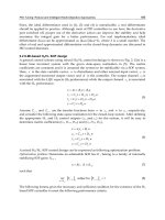
The inductive telemetric system for high temperature measurement is shown schematically
in Figure 10. On the left side of the figure a diagram of the inductive telemetric system is
reported: the sensing element that consists of a planar inductor and a MEMS sensor is

placed in an oven, while outside, separated by a window of tempered glass with a thickness
of 8 mm, there is the readout inductor. The readout inductor was positioned axially to the
hybrid sensor at about one centimetre to the hybrid sensor inside the chamber, while
outside the readout was connected to the impedance analyzer. The two inductors represent
an inductive telemetric system.

InductiveTelemetricMeasurementSystemsforRemoteSensing 357

INTERDIGITATED
CAPACITOR
PLANAR
INDUCTOR
READOUT
INDUCTOR
HARSH
ENVIRONMENT
READOUT
UNIT
HYBRID
TELEMETRIC MEMS
HARSH
ENVIRONMENT
READOUT
UNIT
INTERDIGITATED
CAPACITOR
PLANAR

INDUCTOR
S
T
PLANAR INDUCTOR WIRES

Fig. 10. The inductive telemetric system for high temperature measurement.

The planar inductor, reported on the right, has been obtained by a laser micro-cutting of a
layer of conductive thick films (Du Pont QM14) screen printed over an alumina substrate (50
mm x 50 mm x 0.63 mm). The micro-cutting process consists of a material ablation by a laser.
The inductor has the external diameter of 50 mm, 120 windings each of about 89 μm width
and spaced 75 μm from the others: an enlargement is reported below on the left of Figure 10.
The readout inductor is a planar spiral; it has been realized by a photolithographic
technology on a high-temperature substrate (85N commercialized by Arlon). The readout
inductor has 25 windings, each of 250 μm width and spaced 250 μm from the others. The
internal diameter is 50 mm wide.
The experimental apparatus is schematically reported in Figure 11 and consists of an oven,
three Fluke multimeters, three Pt100 references, two impedance analyzers, a PC and a power
interface. In the measurement chamber (in the centre of the figure) an IR heater of 500 W
rises the temperature up to 350 °C. Three Pt100 thermo-resistances (only one is shown in the
Figure) measure the internal temperature in three different points, and each one is
connected to a multimeter (Fluke 8840A). The three values are used to assure that the
temperature is uniformly distributed.
A Personal Computer, over which runs a developed LabVIEW™ virtual-instrument,
monitors the temperature inside the oven and controls the IR heater by turning alternatively
on and off the power circuit. Two MEMS sensors are placed in the oven. The first one is
directly connected to the impedance analyzer (HP4194A) to measure its capacitance; the
second one is connected to the external readout inductor for the telemetric measurement.
The experimental measurement has been conducted to a temperature up to 330 °C in a
temperature-controlled measurement oven.

AdvancesinMeasurementSystems358

Pt100
PERSONAL
COMPUTER
POWER
INTERFACE
READOUT
INDUCTOR
HYBRID
MEMS
HEATER
IEEE-488
IEEE-488
IEEE-488
FLUKE
8840A
HP4194A
HP4194A

Fig. 11. A diagram of the experimental setup.

140
160
180
200
220
240
1.0 1.3 1.6 1.9 2.2 2.5

|Z|[Ω]
Frequency[MHz]
52°C
60°C
91°C
121°C
153°C
182°C
212°C
241°C
271°C
298°C
331°C
40
48
56
64
72
80
1.0 1.3 1.6 1.9 2.2 2.5
PhaseZ[deg]
Frequency[MHz]
52°C 60°C 91°C 121°C
153°C 182°C 212°C 241°C
271°C 298°C 331°C
(a)
(b)
f
ra
f

a

Fig. 12. Modulus (a) and phase (b) of the hybrid MEMS measured with the impedance
analyzer at different temperatures.
InductiveTelemetricMeasurementSystemsforRemoteSensing 359

In Figure 12 modulus (a) and phase (b) diagrams of the impedance, as measured by the
impedance analyzer at the readout terminal, for different temperatures are reported. The
frequency interval of the abscissa has been chosen to make visible he resonant frequencies
f
ra
, f
a
. As expected an increasing in temperature generates a decreasing of the values of the
resonant frequencies, since the sensor capacitance value increases.

TEMP.
[°C]
f
ra

[MHz]
f
a
[MHz]
f
rb

[MHz]
52

1.9323 2.2904 4.9825
60
1.9120 2.2760 4.9883
91
1.8125 2.1866 4.9853
121
1.7348 2.1005 4.9783
153
1.6625 2.0146 4.9903
182
1.6308 1.9710 4.9928
212
1.6040 1.9414 4.9943
241
1.5828 1.9156 5.0053
271
1.5580 1.8918 5.0255
298
1.5328 1.8557 5.0285
301
1.5243 1.8798 5.0485
331
1.5130 1.8386 5.0463
Table. 1. Frequencies values of f
ra
, f
rb
and f
a
measured for different temperatures.

In Table 1, f
ra
, f
rb
and f
a
values are reported. The two frequencies f
ra
, f
a
, shown also in Figure
12, move down in frequency with increasing temperature as expected. The third frequency
f
rb
is sensitive to temperature, but less than the previous two.

Fig. 13. Sensor’s capacitance is reported as a function of the temperature.
22
24
26
28
30
32
34
36
38
40
30 60 90 120 150 180 210 240 270 300 330 360

Capacitance[pF]
Temperature[°C]
3‐Resonances
HP4194A
Interp.HP4194A
AdvancesinMeasurementSystems360

Fig. 14. Sensor’s capacitance is reported as a function of the temperature.

In Figure 13 the sensor’s capacitance is reported as a function of the temperature: cross
points are the values directly measured on the sensor terminals, while the triangle are
values calculated using the 3-Resonances method and measuring the impedance from the
external inductor terminals. The straight line represents the linear interpolation of the data
obtained by the impedance analyzer and it is reached as reference line. The calculated
values using the 3-Resonances method (Figure 13) shows a quasi linear behaviour of the
sensor: the maximum deviation is about 1.61 pF. Same consideration can be done for the
data obtained using the Min-phase method: the maximum deviation is about 2.15 pF; a
comparison is shown in Figure 14. Then, both the values calculated with the two methods
are closely to the reference one measured with the impedance analyzer (HP4194A).

Fig. 15. Temperature values measured with the Pt100 and compared with the Min-Phase
and 3-Resonances calculated values.
22
24
26
28
30
32

34
36
38
40
30 60 90 120 150 180 210 240 270 300 330 360
Capacitance[pF]
Temperature[°C]
Min‐Phase
HP4194A
Interp.HP4194A
30
70
110
150
190
230
270
310
350
0 2 4 6 8 10 12
Temperature[°C]
Time[hour]
Min‐Phase
3‐Resonances
Pt100
InductiveTelemetricMeasurementSystemsforRemoteSensing 361

In Figure 15 the temperatures measured with the reference sensor (Pt100) are compared
with the values calculated by the Min-Phase and 3-Resonances methods. The temperature
values are obtained using the sensitivity of about 54.6 fF/°C, calculated using the linear

interpolation previously reported. Figure 15 shows a good agreement of the temperature
values during both the heating and the cooling process. The hybrid MEMS follows the trend
of the temperature signal that it has estimated of about 1.9 °C/min and 0.6 °C/min during
the heating and cooling process, respectively.

5. An Inductive Telemetric System for Relative Humidity Measurements

This paragraph describes a telemetric system to measure the relative humidity (RH). A
telemetric system can be useful in hermetic environments since the measurement can be
executed without violating the integrity of the protected environment.
The telemetric system presented here has an interesting characteristic: the sensing inductor
does not have any transducer, since the parasitic capacitance of the sensing inductor is the
sensing element. In this paragraph, the measurement technique of the three resonances has
been used to analyse the effectiveness of compensation in the distance.
In this system the sensing inductor consists only of the planar inductor over which a
polymer, humidity sensitive, is deposited. This polymer is sensitive to the humidity and
changes its dielectric permittivity causing a variation of the inductor parasitic capacitance.
The terminals of the readout inductor are the input of the conditioning electronics reported
in paragraph 3. The electronics measures the frequency resonances, extracts the
corresponding capacitance values and compensates the distance variation as well.

WIRES

SENSING
POLYMER
SENSING
INDUCTOR

Fig. 16. The inductive sensor, on which a polymer, humidity sensitive, is deposited.

In Figure 16 the passive inductive sensor is reported, which is a standalone planar inductor,
fabricated in PCB technology of 25 windings with an external diameter of 50 mm covered by
polyethylene glycol (PEG). Polyethylene glycol (PEG) was chosen for the highest sensitivity,
but other polymer sensitive to the RH can be used as well. Differently from the others tested
AdvancesinMeasurementSystems362

in laboratory, this polymer is soluble in water: this characteristic influences the sensitivity
positively, but increases the hysteresis as well. Its dielectric constant changes from 2.2 to 4
and depends on temperature and humidity. The characteristics of the telemetric system have
been verified with a humidity-controlled hermetical measurement chamber changing also
the distance between the sensing and readout inductors.

READOUT
SENSOR
EXHAUST
HUMIDITY
CONTROL
MEASUREMENT
CIRCUIT
REFERENCE
HYGROMETER

HP4194A

Fig. 17. Block scheme of the experimental system.

In Figure 17 the experimental apparatus to test the telemetric system is schematically
represented. The sensor is positioned inside a Plexiglas chamber, which is used as a hermetic

container for the damp air. Two pipes are linked to the measurement chamber, one of which
introduces controlled damp air. The damp air is produced by a system that compounds dry air
and wet air using two flux-meters. The time required to reach the new RH value is about one
hour and half. In the chamber there is a hygrometric sensor (HIH-3610 Honeywell) for
reference measurements. The inductances are positioned parallel and their axes are coincident.
The distance of the readout from the sensor is controlled by a micrometric screw with
resolution 10 µm and runs up to 25 mm. The terminals of the readout inductor are connected
to the input of the conditioning electronics or, alternatively, to the input of the impedance
analyzer. The use of the impedance analyzer is used only for test purposes. The proposed
electronics
measures the frequency resonances and calculates the corresponding capacitance
values according to formula (28). The formula compensates the distance variation as well.
The capacitance values measured at a distance of 20 mm between the readout and sensing
inductors the calculated capacitance values are reported in Figure 18: the square point are
the value obtained by the electronics while the values obtained using the impedance
analyzer (HP4194A) are reported as cross points. All the measurement points are a function
of the RH values as measured by the reference sensor. Interpolating the two sets of
measurement data the maximum difference between the two curves is less than 15 fF,
corresponding to less than 8% of the capacitance measurement range.
In Figure 19 the capacitance values as a function of distance are reported over a distance
variation from 15 to 30 mm. The maximum variation of the capacitance is, in the worst case,
limited to 20 fF corresponding to about of 1% of FS for each millimetre of distance variation.
InductiveTelemetricMeasurementSystemsforRemoteSensing 363

Fig. 18. The calculated capacitance values as a function of RH and for different distance
values.

Fig. 19. The capacitance values as a function of distance for different RH values.

6. Conclusion

Inductive telemetric systems offer solutions to specific applications where the measurement
data should be acquired in environments that are incompatible with the active electronics or
are inaccessible. They also work without batteries, consequently reducing the problem of
environmental impact. The general architecture of an inductive telemetric system, the
measurement techniques, commonly used, were presented, along with the description of
developed telemetric systems applied in harsh or hermetic environments. Two examples of
passive inductive telemetric systems were reported, the first one for humidity
measurements which presents a distance interval of about 30 mm and the possibility to
compensate the distance variation. The second one can measure high temperatures with a
maximum limit of about 350 °C, guaranteeing the inviolability of the harsh environment.
1.7
1.72
1.74
1.76
1.78
1.8
1.82
1.84
1.86
1.88
1.9
10 20 30 40 50 60 70 80 90 100
Sensor Capacitance C'
S
[pF]
RH [%]
20 mm (Electronics)

20 mm (HP4194A)
Interp. HP4194A
Interp. Electronics
1.69
1.73
1.77
1.81
1.85
1.89
15 17.5 20 22.5 25 27.5 30
Sensor Capacitance C'
S
[pF]
Distance [mm]
RH=15.5 RH=56.5 RH=66
RH=73.6 RH=85.3 RH=90
AdvancesinMeasurementSystems364

7. References

Akar, O.; Akin, T. & Najafi, K. (2001). A wireless batch sealed absolute capacitive pressure
sensor, Sensors and Actuators A, Vol. 95 pp. 29-38.
Andò, B.; Baglio, S.; Pitrone, N.; Savalli, N. & Trigona, C. (2008). Bent beam MEMS
temperature sensors for contactless measurements in harsh environments,
Proceedings of IEEE I2MTC08, Victoria BC, Canada, pp. 1930-1934.
Birdsell, E. & Allen, M.G.; (2006). Wireless Chemical Sensors for High Temperature
environments, Tech. Dig. Solid-State Sensor, Actuator, and Microsystems Workshop,
Hilton Head Island, SC, USA, pp. 212-215.
Fonseca, M.A.; Allen, M.G.; Kroh, J. & White, J. (2006). Flexible wireless passive pressure
sensors for biomedical applications, Tech. Dig. Solid State Sensor, Actuator, and

Microsystems Workshop, Hilton Head Island, South Carolina, June 4-8, pp. 37-42.
Fonseca, M.A.; English, J.M.; Von Arx, M. & Allen, M.G. (2002). Wireless micromachined
ceramic pressure sensor for high temperature applications, Journal of Microel.
Systems, Vol. 11, pp. 337-343.
Hamici, Z.; Itti, R. & Champier, J. (1996). A high-efficiency power and data transmission
system for biomedical implanted electronic device, Measurement Science and
Technology, Vol. 7, pp. 192-201.
Harpster, T.; Stark, B. & Najafi, K. (2002). A passive wireless integrated humidity sensor,
Sensors and Actuators A, Vol. 95, pp. 100-107.
Jia, Y.; Sun, K.; Agosto, F.J. & Quinones, M.T. (2006). Design and characterization of a
passive wireless strain sensor, Measurement Science and Technology, Vol. 17, pp. 2869-
2876.
Marioli, D.; Sardini, E.; Serpelloni, M. & Taroni, A. (2005). A new measurement method for
capacitance transducers in a distance compensated telemetric sensor system,
Measurement Science and Technology, Vol. 16, pp. 1593-1599.
Ong, K.G.; Grimes, C.A.; Robbins, C.L. & Singh, R.S. (2001). Design and application of a
wireless, passive, resonant-circuit environmental monitoring sensor, Sensors and
Actuators A, Vol. 93, pp. 33-43.
Schnakenberg, U.; Walter, P.; Vom Bogel G.; Kruger C.; Ludtke-Handjery H.C.; Richter H.A.;
Specht W.; Ruokonen P. & Mokwa W. (2000). Initial investigations on systems for
measuring intraocular pressure, Sensors and Actuators A, Vol. 85, pp. 287-291.
Takahata, K. & Gianchandani, Y.B. (2008). A micromachined capacitive pressure sensor
using a cavity-less structure with bulk-metal/elastomer layers and its wireless
telemetry application, Sensors, Vol. 8, pp. 2317-2330.
Tan, E.L.; Ng, W.N.; Shao, R.; Pereles, B.D. & Ong, K.G. (2007). A wireless, passive sensor for
quantifying packaged food quality, Sensors, Vol. 7, pp. 1747-1756.
Todoroki, A.; Miyatani, S. & Shimamura, Y. (2003). Wireless strain monitoring using
electrical capacitance change of tire: part II-passive, Smart Materials and Structures,
Vol. 12, pp. 410-416.
Wang, Y.; Jia, Y.; Chen, Q. & Wang, Y. (2008). A Passive Wireless Temperature Sensor for

Harsh Environment Applications, Sensors, Vol. 8, pp. 7982-7995.

MeasurementofVoltageFlicker:ApplicationtoGrid-connectedWindTurbines 365
Measurement of Voltage Flicker: Application to Grid-connected Wind
Turbines
J.J.GutierrezandJ.RuizandA.LazkanoandL.A.Leturiondo
0
Measurement of Voltage Flicker:
Application to Grid-connected
Wind Turbines
J.J. Gutierrez and J. Ruiz and A. Lazkano and L.A. Leturiondo
University of the Basque Country
Spain
1. Introduction
Electric power is an essential commodity for most industrial, commercial and domestic pro-
cesses. As a product, electric power must be of an acceptable quality, to guarantee the correct
behavior of the equipment connected to the power distribution system. Low-frequency con-
ducted disturbances are the main factors that can compromise power quality. The IEC 61000-
2-1 standard classiﬁes low-frequency conducted disturbances in the following ﬁve groups:
harmonics and interharmonics, voltage dips and short supply interruptions, voltage unbal-
ance, power frequency variations and voltage ﬂuctuations or ﬂicker.
Voltage ﬂuctuations are deﬁned as cyclic variations in voltage with amplitude below 10% of
the nominal value. Most of the connected equipment is not affected by voltage ﬂuctuations,
but these ﬂuctuations may cause changes in the illumination intensity of light sources, known
as ﬂicker. Flicker may produce a very unpleasant visual sensation, leading to complaints from
utility customers. The annoyance level depends on the type of lamp and amplitude, frequency
and duration of the voltage ﬂuctuations. Its precise quantiﬁcation is a complex task that must
be statistically approached to characterize adequately the perception of a large number of peo-
ple. A ﬂickermeter must characterize the behavior of the lamp-eye-brain set that represents
most people and must provide an indication of the discomfort, or ﬂicker severity. In 1986, The

International Electrotechnical Commission (IEC) published the ﬁrst standard describing the
functional and design speciﬁcations for the measurement of ﬂicker.
The main sources of ﬂicker are large industrial loads, such as arc furnaces, or smaller loads
with regular duty cycles, such as welding machines or electric boilers. However, from the
point of view of power generation, ﬂicker as a result of wind turbines has gained attention in
recent years. Rapid variations in wind speed produce ﬂuctuating power, which can lead to
voltage ﬂuctuations at the point of common coupling (PCC), which in turn generate ﬂicker.
The IEC 61400-21 standard establishes the procedures for measuring and assessing the power
quality characteristics of grid-connected wind turbines. The section dedicated to ﬂicker pro-
poses a complex model for calculating the ﬂicker coefﬁcient that characterizes a wind turbine.
This coefﬁcient must be estimated from the current and voltage time series obtained for differ-
ent wind conditions. The wind turbine being tested is usually connected to a medium-voltage
network, having other ﬂuctuating loads that may cause signiﬁcant voltage ﬂuctuations. In
addition, the voltage ﬂuctuations imposed by the wind turbine depend on the characteristics
15
AdvancesinMeasurementSystems366
of the grid conditions. The most relevant block of the model is responsible for simulating the
voltage ﬂuctuations on a ﬁctitious grid with no source of ﬂicker other than the wind turbine.
This chapter is organized in two related sections. The ﬁrst section deals with the IEC ﬂicker-
meter. First, the main research enabling modeling of the lamp-eye-brain set is summarized.
A description of the IEC 61000-4-15 standard follows, as well as a detailed account of a high-
precision digital implementation of the ﬂickermeter, after which the ability of the IEC ﬂicker-
meter to assess the actual annoyance produced by ﬂicker in people is critically analyzed. This
analysis is based on ﬁeld measurements obtained from analytically generated test signals and
subjective experimental data obtained from a small group of people. In the second section, the
IEC ﬂickermeter is used to characterize ﬂicker caused by wind turbines. The section contains
a detailed description of the part of the IEC-61400-21 standard dedicated to ﬂicker, together
with a critical analysis of the different methods used to solve the ﬁctitious grid. The chap-
ter concludes by analyzing how the errors in the estimation of the ﬁctitious grid affect the
calculation of ﬂicker severity.

2. Measurement of ﬂicker
2.1 Historical perspective
Flicker is deﬁned as the variation in the luminosity produced in a light source because of
ﬂuctuations in the supply voltage. Fig. 1 shows an example of rectangular ﬂuctuation at a
frequency of 8.8 Hz and an amplitude ∆V = 0.4 V (i.e.,
∆V
V
= 40 %), which modulates a mains
signal of 50 Hz and amplitude V = 1 V.
Time (s)
Amplitude (V)
ΔV
V
0
0.05
0.1
0.15
0.2
0.25
0.3
-1
-0.5
0
0.5
0.8
1
1.2
Fig. 1. Example of rectangular ﬂuctuation in voltage supply.
Variations in luminosity can annoy humans. A ﬂicker measuring device or ﬂickermeter must
assess the annoyance, or the ﬂicker severity, caused to people exposed to variations in lumi-

nosity. The measurement of the annoyance caused should be done starting from the supply
voltage of the light source.
It is obvious that the annoyance caused is a subjective phenomenon, related to the sensitivity
of each individual to light ﬂuctuations. In this sense, the measurement of annoyance can
only be performed on a statistical basis; that is, by carrying out experiments involving a large
number of people. A ﬂickermeter has to provide an acceptable model of the behavior of the
lamp-eye-brain set responsible for converting the voltage ﬂuctuations into annoyance.
The voltage ﬂuctuations are converted in the lamp into light ﬂuctuations. The response de-
pends, to a great extent, on its construction, power and nominal voltage. Consequently, in
order to deﬁne the speciﬁcations of a ﬂickermeter, it is necessary to select a suitable reference
lamp. The analysis of the lamp-eye system requires carrying out statistical studies to enable
characterization of the behavior of the human eye when exposed to light ﬂuctuations. Lastly,
the eye-brain set constitutes a complex, nonlinear system, and its neurophysiological study
also requires a statistical basis. Complex characteristics of the brain, such as its memory ca-
pacity and its inertia when faced with consecutive variations in luminosity, must be modeled.
The ﬁrst research into the behavior of the lamp-eye set was carried out by K. Simons (Simons,
1917). More detailed studies on the behavior of the lamp-eye set were carried out by P. Ailleret,
at the end of the 1950s (Ailleret, 1957). These experiments were based on various subjective
tests on representative groups of people, and they analyzed the behavior of the lamp-eye set
with various lamp types. They demonstrated that the lamp-eye system has a band-pass-type
response with maximum sensitivity around 10 Hz for incandescent lamps. This work also
deﬁned the response of the incandescent lamp under small variations in voltage:
∆L
L
n
= γ
∆V
V
n
, (1)

where V
n
represents the root mean square (rms) value of the nominal voltage, L
n
is its cor-
responding luminosity and γ is a proportionality constant. This expression leads to the con-
clusion that the level of annoyance calculated in ﬂicker measurement must be proportional
to the relative level of voltage ﬂuctuation. That is, double the amplitude of voltage ﬂuctua-
tion corresponds to double the amplitude of luminosity ﬂuctuation and, therefore, double the
annoyance.
In a second experiment, P. Ailleret related the annoyance to the amplitude of the ﬂuctuation
and its duration. The results demonstrated that the annoyance depends on the product of two
factors, the duration and square of the amplitude, according to the following expression:
Annoyance
= f (L
2
·t) , (2)
where L represents the ﬂuctuation amplitude and t the duration.
That is, a continuous variation in luminosity with a speciﬁc voltage amplitude and frequency,
during a particular interval, provokes the same annoyance as three-quarters of the interval
without ﬂuctuation and a quarter of the interval with double the amplitude.
Finally, P. Ailleret studied the combination of annoyance provoked by light ﬂuctuations with
different frequencies. He demonstrated that the combination of the amplitudes follows a
quadratic law. If the annoyance at frequency f
1
has equivalent amplitude, L
1
, at 20 Hz, and
at another frequency f
2

it has equivalent amplitude L
2
, the overall effect of the combined
presence of the two frequencies is given by:
∆L
=

∆L
2
1
+ ∆L
2
2
(3)
In parallel with the previous works, H. de Lange considered that the ambient luminosity is
an important factor in the evaluation of the annoyance and characterized the response of the
human eye by taking into account the inﬂuence of the illumination level of the retina. Fig. 2
shows the relation between the amplitude of the luminous ﬂuctuation and the average ambi-
ent luminosity against frequency, at the perceptibility threshold (de Lange, 1961) for an incan-
descent lamp. The variation of this relationship with frequency is provided on a logarithmic
scale for different illuminations of the retina. From the ﬁgure, it can be deduced that for high
MeasurementofVoltageFlicker:ApplicationtoGrid-connectedWindTurbines 367
of the grid conditions. The most relevant block of the model is responsible for simulating the
voltage ﬂuctuations on a ﬁctitious grid with no source of ﬂicker other than the wind turbine.
This chapter is organized in two related sections. The ﬁrst section deals with the IEC ﬂicker-
meter. First, the main research enabling modeling of the lamp-eye-brain set is summarized.
A description of the IEC 61000-4-15 standard follows, as well as a detailed account of a high-
precision digital implementation of the ﬂickermeter, after which the ability of the IEC ﬂicker-
meter to assess the actual annoyance produced by ﬂicker in people is critically analyzed. This
analysis is based on ﬁeld measurements obtained from analytically generated test signals and

subjective experimental data obtained from a small group of people. In the second section, the
IEC ﬂickermeter is used to characterize ﬂicker caused by wind turbines. The section contains
a detailed description of the part of the IEC-61400-21 standard dedicated to ﬂicker, together
with a critical analysis of the different methods used to solve the ﬁctitious grid. The chap-
ter concludes by analyzing how the errors in the estimation of the ﬁctitious grid affect the
calculation of ﬂicker severity.
2. Measurement of ﬂicker
2.1 Historical perspective
Flicker is deﬁned as the variation in the luminosity produced in a light source because of
ﬂuctuations in the supply voltage. Fig. 1 shows an example of rectangular ﬂuctuation at a
frequency of 8.8 Hz and an amplitude ∆V = 0.4 V (i.e.,
∆V
V
= 40 %), which modulates a mains
signal of 50 Hz and amplitude V = 1 V.
Time (s)
Amplitude (V)
ΔV
V
0
0.05
0.1
0.15
0.2
0.25
0.3
-1
-0.5
0
0.5

0.8
1
1.2
Fig. 1. Example of rectangular ﬂuctuation in voltage supply.
Variations in luminosity can annoy humans. A ﬂicker measuring device or ﬂickermeter must
assess the annoyance, or the ﬂicker severity, caused to people exposed to variations in lumi-
nosity. The measurement of the annoyance caused should be done starting from the supply
voltage of the light source.
It is obvious that the annoyance caused is a subjective phenomenon, related to the sensitivity
of each individual to light ﬂuctuations. In this sense, the measurement of annoyance can
only be performed on a statistical basis; that is, by carrying out experiments involving a large
number of people. A ﬂickermeter has to provide an acceptable model of the behavior of the
lamp-eye-brain set responsible for converting the voltage ﬂuctuations into annoyance.
The voltage ﬂuctuations are converted in the lamp into light ﬂuctuations. The response de-
pends, to a great extent, on its construction, power and nominal voltage. Consequently, in
order to deﬁne the speciﬁcations of a ﬂickermeter, it is necessary to select a suitable reference
lamp. The analysis of the lamp-eye system requires carrying out statistical studies to enable
characterization of the behavior of the human eye when exposed to light ﬂuctuations. Lastly,
the eye-brain set constitutes a complex, nonlinear system, and its neurophysiological study
also requires a statistical basis. Complex characteristics of the brain, such as its memory ca-
pacity and its inertia when faced with consecutive variations in luminosity, must be modeled.
The ﬁrst research into the behavior of the lamp-eye set was carried out by K. Simons (Simons,
1917). More detailed studies on the behavior of the lamp-eye set were carried out by P. Ailleret,
at the end of the 1950s (Ailleret, 1957). These experiments were based on various subjective
tests on representative groups of people, and they analyzed the behavior of the lamp-eye set
with various lamp types. They demonstrated that the lamp-eye system has a band-pass-type
response with maximum sensitivity around 10 Hz for incandescent lamps. This work also
deﬁned the response of the incandescent lamp under small variations in voltage:
∆L
L

n
= γ
∆V
V
n
, (1)
where V
n
represents the root mean square (rms) value of the nominal voltage, L
n
is its cor-
responding luminosity and γ is a proportionality constant. This expression leads to the con-
clusion that the level of annoyance calculated in ﬂicker measurement must be proportional
to the relative level of voltage ﬂuctuation. That is, double the amplitude of voltage ﬂuctua-
tion corresponds to double the amplitude of luminosity ﬂuctuation and, therefore, double the
annoyance.
In a second experiment, P. Ailleret related the annoyance to the amplitude of the ﬂuctuation
and its duration. The results demonstrated that the annoyance depends on the product of two
factors, the duration and square of the amplitude, according to the following expression:
Annoyance
= f (L
2
·t) , (2)
where L represents the ﬂuctuation amplitude and t the duration.
That is, a continuous variation in luminosity with a speciﬁc voltage amplitude and frequency,
during a particular interval, provokes the same annoyance as three-quarters of the interval
without ﬂuctuation and a quarter of the interval with double the amplitude.
Finally, P. Ailleret studied the combination of annoyance provoked by light ﬂuctuations with
different frequencies. He demonstrated that the combination of the amplitudes follows a
quadratic law. If the annoyance at frequency f

1
has equivalent amplitude, L
1
, at 20 Hz, and
at another frequency f
2
it has equivalent amplitude L
2
, the overall effect of the combined
presence of the two frequencies is given by:
∆L
=

∆L
2
1
+ ∆L
2
2
(3)
In parallel with the previous works, H. de Lange considered that the ambient luminosity is
an important factor in the evaluation of the annoyance and characterized the response of the
human eye by taking into account the inﬂuence of the illumination level of the retina. Fig. 2
shows the relation between the amplitude of the luminous ﬂuctuation and the average ambi-
ent luminosity against frequency, at the perceptibility threshold (de Lange, 1961) for an incan-
descent lamp. The variation of this relationship with frequency is provided on a logarithmic
scale for different illuminations of the retina. From the ﬁgure, it can be deduced that for high
AdvancesinMeasurementSystems368
levels of illumination, the frequency response of the optical system behaves as a band-pass ﬁl-
ter, with a maximum sensitivity at a frequency of 8.8 Hz, making it the reference of sensitivity

for human visual perception of ﬂicker.
Frequency (Hz)
r (%)
* 4.3 phot ons
+ 43 photons
x 430 photons
1 2 3 4 5 10 20
30
40 50
100
30
10
3
1
Fig. 2. Frequency characteristics of the human optical system at the threshold of perception
for different illumination levels. Source: (de Lange, 1952).
Once the lamp-eye set had been studied, to complete the model of perception, it was essential
to analyze the behavior of the eye-brain system. During the 1970s, a series of experiments were
conducted, aimed at mathematical modeling of the neurophysiological processes caused by
light ﬂuctuations.
The ﬁrst such research, undertaken by C. Rashbass, obtained the lowest intensity at which the
rectangular changes of luminance of a speciﬁc duration are perceptible (Rashbass, 1970). The
results demonstrated that the relative intensity decreases with increasing ﬂash duration, with
a minimum at 64 ms, supporting the band-pass characteristic postulated by H. de Lange and
Ailleret.
In the second study, C. Rashbass combined two ﬂashes of the same duration but with inten-
sities that were not necessarily the same. The results demonstrated that the response to any
combination of two intensities obeyed a quadratic law, which could be modeled using three
elements:
a. a band-pass ﬁlter coinciding with the one previously used by H. de Lange to model eye

behavior;
b. a second element reproducing the quadratic response of the system, which is modeled
using a squaring circuit; and
c. a third element to model the effect of the brain’s memory using a ﬁrst-order band-pass
ﬁlter and a time constant between 150 and 250 ms
1
.
Fig. 3 shows the analog model of the eye-brain set produced from Rashbass’ experiments. This
model constitutes the nucleus of the current speciﬁcation of the IEC ﬂickermeter (IEC-61000-
4-15, 2003; IEC-868, 1986).
1
This constant was deﬁnitively ﬁxed at 300 ms starting from the studies of Koenderink and Van Doorn
(Koenderink & van Doorn, 1974).
Input
Light
ﬂutuations
1
Weighting ﬁlter
2
Squaring circuit
3
1
st
order
low-pass ﬁlter
Output
Instantane ous
ﬂicker sensation
Elements of the model
r(t)

f
t
f
s(t)
Fig. 3. Model of visual perception (eye-brain set) based on studies by H. de Lange and C.
Rashbass. Source: (UIE, 1992).
2.2 Description of the IEC ﬂickermeter
At the end of the 1970s, the UIE
2
perturbations working group started to prepare a speciﬁ-
cation for the measurement of ﬂicker that was universally accepted. The ﬁrst results of this
work were presented to the international community at the 1984 UIE congresses (Nevries,
1984). The deﬁnitive version was standardized in 1986 through the IEC 868 standard (IEC-
868, 1986), which provided the functional and design speciﬁcations of a ﬂicker measuring
device. Currently, the standard containing the speciﬁcations of the ﬂickermeter is IEC 61000-
4-15 (IEC-61000-4-15, 2003).
Fig. 4 shows the block diagram deﬁned by IEC 61000-4-15. The simulation of the response
of the lamp-eye-brain system is carried out in the ﬁrst four blocks, based on the physiolog-
ical experiments described previously. In addition, the standard requires integration of the
sensation experienced by the observer during a speciﬁc period in a single value. Block 5 is
responsible for this, through a statistical evaluation of the output from block 4.
u(t)
BLOCK 1
INPUT
VOLTAGE
ADAPTOR
BLOCK 2
QUADRATIC
DEMODULATOR
BLOCK 3

0.05 35 8.8
RANGE
SELECTOR
DEMODULATION AND WEIGHTING FILTERS
BLOCK 4
SQUARING
MULTIPLIER
+
SLIDING
LOW-PASS
FILTER
BLOCK 5
STATISTICAL
EVALUATION
P
st
Fig. 4. Block diagram of the ﬂickermeter speciﬁed in the IEC 61000-4-15 standard.
Next, a brief description is given of each block shown in Fig. 4 for 50 Hz systems. The main
characteristics of a high-precision digital implementation developed as a reference for the
results found in the rest of this chapter are described in the following sections.
2.2.1 Block 1: Input voltage adaptor
Given that the ﬂicker measurement must be made from the relative ﬂuctuations in voltage,
expressed in percentages, it is necessary to guarantee the independence of the input voltage
measurement. In this block, the input is scaled with respect to its average value. This op-
eration can be done through automatic adjustment of the gain at the rms value of the input
voltage, with a constant time of 1 min.
2
International Union for Electrical Applications.
MeasurementofVoltageFlicker:ApplicationtoGrid-connectedWindTurbines 369
levels of illumination, the frequency response of the optical system behaves as a band-pass ﬁl-

ter, with a maximum sensitivity at a frequency of 8.8 Hz, making it the reference of sensitivity
for human visual perception of ﬂicker.
Frequency (Hz)
r (%)
* 4.3 phot ons
+ 43 photons
x 430 photons
1 2 3 4 5 10 20
30
40 50
100
30
10
3
1
Fig. 2. Frequency characteristics of the human optical system at the threshold of perception
for different illumination levels. Source: (de Lange, 1952).
Once the lamp-eye set had been studied, to complete the model of perception, it was essential
to analyze the behavior of the eye-brain system. During the 1970s, a series of experiments were
conducted, aimed at mathematical modeling of the neurophysiological processes caused by
light ﬂuctuations.
The ﬁrst such research, undertaken by C. Rashbass, obtained the lowest intensity at which the
rectangular changes of luminance of a speciﬁc duration are perceptible (Rashbass, 1970). The
results demonstrated that the relative intensity decreases with increasing ﬂash duration, with
a minimum at 64 ms, supporting the band-pass characteristic postulated by H. de Lange and
Ailleret.
In the second study, C. Rashbass combined two ﬂashes of the same duration but with inten-
sities that were not necessarily the same. The results demonstrated that the response to any
combination of two intensities obeyed a quadratic law, which could be modeled using three
elements:

a. a band-pass ﬁlter coinciding with the one previously used by H. de Lange to model eye
behavior;
b. a second element reproducing the quadratic response of the system, which is modeled
using a squaring circuit; and
c. a third element to model the effect of the brain’s memory using a ﬁrst-order band-pass
ﬁlter and a time constant between 150 and 250 ms
1
.
Fig. 3 shows the analog model of the eye-brain set produced from Rashbass’ experiments. This
model constitutes the nucleus of the current speciﬁcation of the IEC ﬂickermeter (IEC-61000-
4-15, 2003; IEC-868, 1986).
1
This constant was deﬁnitively ﬁxed at 300 ms starting from the studies of Koenderink and Van Doorn
(Koenderink & van Doorn, 1974).
Input
Light
ﬂutuations
1
Weighting ﬁlter
2
Squaring circuit
3
1
st
order
low-pass ﬁlter
Output
Instantane ous
ﬂicker sensation
Elements of the model

r(t)
f
t
f
s(t)
Fig. 3. Model of visual perception (eye-brain set) based on studies by H. de Lange and C.
Rashbass. Source: (UIE, 1992).
2.2 Description of the IEC ﬂickermeter
At the end of the 1970s, the UIE
2
perturbations working group started to prepare a speciﬁ-
cation for the measurement of ﬂicker that was universally accepted. The ﬁrst results of this
work were presented to the international community at the 1984 UIE congresses (Nevries,
1984). The deﬁnitive version was standardized in 1986 through the IEC 868 standard (IEC-
868, 1986), which provided the functional and design speciﬁcations of a ﬂicker measuring
device. Currently, the standard containing the speciﬁcations of the ﬂickermeter is IEC 61000-
4-15 (IEC-61000-4-15, 2003).
Fig. 4 shows the block diagram deﬁned by IEC 61000-4-15. The simulation of the response
of the lamp-eye-brain system is carried out in the ﬁrst four blocks, based on the physiolog-
ical experiments described previously. In addition, the standard requires integration of the
sensation experienced by the observer during a speciﬁc period in a single value. Block 5 is
responsible for this, through a statistical evaluation of the output from block 4.
u(t)
BLOCK 1
INPUT
VOLTAGE
ADAPTOR
BLOCK 2
QUADRATIC
DEMODULATOR

BLOCK 3
0.05 35 8.8
RANGE
SELECTOR
DEMODULATION AND WEIGHTING FILTERS
BLOCK 4
SQUARING
MULTIPLIER
+
SLIDING
LOW-PASS
FILTER
BLOCK 5
STATISTICAL
EVALUATION
P
st
Fig. 4. Block diagram of the ﬂickermeter speciﬁed in the IEC 61000-4-15 standard.
Next, a brief description is given of each block shown in Fig. 4 for 50 Hz systems. The main
characteristics of a high-precision digital implementation developed as a reference for the
results found in the rest of this chapter are described in the following sections.
2.2.1 Block 1: Input voltage adaptor
Given that the ﬂicker measurement must be made from the relative ﬂuctuations in voltage,
expressed in percentages, it is necessary to guarantee the independence of the input voltage
measurement. In this block, the input is scaled with respect to its average value. This op-
eration can be done through automatic adjustment of the gain at the rms value of the input
voltage, with a constant time of 1 min.
2
International Union for Electrical Applications.
AdvancesinMeasurementSystems370

In our reference implementation, the input signal is scaled to an internal reference value pro-
portional to the 1 min rms value, using a half-cycle sliding window.
2.2.2 Block 2: Quadratic demodulator
Voltage ﬂuctuations normally appear as a modulation in amplitude of the fundamental com-
ponent. Thus, the input to block 2 can be understood as a modulated signal with a sinusoidal
carrier of 50 Hz. Block 2 is responsible for carrying out the quadratic demodulation of the
input.
The light source chosen by IEC as reference for the construction of the ﬂickermeter is an in-
candescent lamp ﬁlled with inert gas with a spiral tungsten ﬁlament and a nominal power of
60 W at 230 V for 50 Hz systems, and 120 V for 60 Hz systems.
The processing required by this block is simply to square the samples from the signal obtained
in block 1. This operation generates a signal containing frequency components corresponding
to the ﬂuctuation in luminosity and other frequencies that have to be suitably eliminated.
2.2.3 Block 3: Demodulation and weighting ﬁlters
To select the frequency components that generate ﬂicker from the output of block 2, it is nec-
essary to suppress the continuous and 100 Hz components generated in the demodulation
process. This is done through the demodulation ﬁlters, which consist of the cascade connec-
tion of:
a. a ﬁrst-order high-pass ﬁlter with a cutoff frequency of 0.05 Hz; and
b. a sixth-order low-pass Butterworth ﬁlter with a cutoff frequency of 35 Hz, which intro-
duces an attenuation of 55 dB at 100 Hz.
The human eye has a selective, frequency-dependent behavior toward variations in luminos-
ity. For this reason, the second stage of ﬁltering consists of a weighted band-pass ﬁlter that
follows the frequency response of the lamp-eye set. This ﬁlter is based on the threshold curve
of perceptibility obtained experimentally by H. de Lange (de Lange, 1952; 1961). The standard
provides the transfer function in the continuous domain of this ﬁlter. With respect to attenua-
tion, at 100 Hz, this ﬁlter adds 37 dB to what has already been achieved using the band-pass
demodulation.
Finally, block 3 contains a measurement scale selector that determines the sensitivity of the
instrument. It modiﬁes the gain depending on the amplitude of the voltage ﬂuctuation to be

measured. The scales, expressed as the relative changes in voltage,
∆V
V
(%), for a sinusoidal
modulation of 8.8 Hz, are 0.5%, 1%, 2%, 5% and 10%, the 20% scale being optional.
For the discrete implementation of the ﬁlters, Inﬁnite Impulse Response (IIR) systems were
selected. The demodulation ﬁlters were designed through the impulsive invariance method,
and the weighting band-pass ﬁlter using bilinear transformation. All the ﬁlters were imple-
mented using the direct-form II transpose.
The reference ﬂickermeter works with sampling frequencies ( f
s
) of 1600, 3200, 6400, 12800 and
25600
samples
s
, and demodulation ﬁlters were designed for these frequencies.
Given that the bandwidth of the output signal of the low-pass demodulation was practically
reduced to 35 Hz, maintaining such high sampling rates is not necessary. For this reason, a
decimation process is implemented at the output of the low-pass demodulation ﬁlter, which
reduces f
s
to f
p
= 800
samples
s
. This decimation process does not require low-pass ﬁltering, as
the signal to be decimated is band limited. In this way, the weighting ﬁlter designed for f
p
is

the same for all the input sampling frequencies.
2.2.4 Block 4: Nonlinear variance estimator
To complete the model of visual perception deﬁned by C. Rashbass, it is necessary to add two
new functions: the modeling of the nonlinear perception of the eye-brain set and the effect of
the brain’s memory. These two functions are introduced using a quadratic multiplier and a
ﬁrst-order sliding low-pass ﬁlter with a time constant of 300 ms.
As for the low-pass ﬁlter in block 3, this ﬁlter has also been designed using the impulsive
invariance method for 800
samples
s
, and it was also implemented in the transposed form of the
direct II form.
The output of this block represents the instantaneous sensation of ﬂicker. It should be stressed
that this signal must not be evaluated as an absolute indicator. On the contrary, it must be
referred to the unit, taking this as the maximum value of the output of this block if the supply
voltage is modulated by a sinusoidal frequency ﬂuctuation of 8.8 Hz and an amplitude 0.25%,
corresponding to the threshold of perceptibility.
2.2.5 Block 5: Statistical evaluation
Block 5 has the aim of assessing the level of annoyance starting with the values of the instan-
taneous sensation of ﬂicker that are exceeded during a certain percentage of the observation
time. It is important to choose a suitable assessment period that is characteristic of the reaction
of an observer confronted with different types of light ﬂuctuations. Because of the disparity in
the characteristics of ﬂicker-generating loads, the standard deﬁnes two observation periods:
a. short term, normally ﬁxed at 10 min, during which short-term ﬂicker severity, P
st
, is
assessed; and
b. long term, usually 2 h, during which long-term ﬂicker severity, P
lt
, is assessed.

It should be noted that the annoyance threshold corresponds to P
st
= 1. When P
st
> 1, the
observer is understood to suffer annoyance; when P
st
< 1, the light ﬂuctuations may be per-
ceivable but not annoying.
2.2.5.1 Evaluation of short-term ﬂicker severity, P
st
Because of the random nature of ﬂicker, it must be assumed that the instantaneous sensation
of ﬂicker may be subject to strong and unpredictable variations. For this reason, not only the
maximum value reached but also the levels exceeded during speciﬁc parts of the observation
period must be taken into account. Therefore, it seems best to design a method based on
a statistical evaluation of the instantaneous sensation. The standard speciﬁes a multipoint
adjustment method according to the following expression:
P
st
=

k
1
P
1
+ k
2
P
2
+ + k

n
P
n
, (4)
where k
n
are weighting coefﬁcients and P
n
are levels corresponding to the percentiles
3
1, 2, . . . , n of the output of block 4. The values k
n
and P
n
were adjusted starting with the
annoyance threshold curve or P
st
= 1 curve, obtained experimentally from a large group of
people undergoing rectangular light ﬂuctuations at more than one change per minute (cpm).
The results providing values lower than 5% for all cases were as follows:
3
Level of instantaneous sensation of ﬂicker that is surpassed during a speciﬁc part of a time period.
MeasurementofVoltageFlicker:ApplicationtoGrid-connectedWindTurbines 371
In our reference implementation, the input signal is scaled to an internal reference value pro-
portional to the 1 min rms value, using a half-cycle sliding window.
2.2.2 Block 2: Quadratic demodulator
Voltage ﬂuctuations normally appear as a modulation in amplitude of the fundamental com-
ponent. Thus, the input to block 2 can be understood as a modulated signal with a sinusoidal
carrier of 50 Hz. Block 2 is responsible for carrying out the quadratic demodulation of the
input.

The light source chosen by IEC as reference for the construction of the ﬂickermeter is an in-
candescent lamp ﬁlled with inert gas with a spiral tungsten ﬁlament and a nominal power of
60 W at 230 V for 50 Hz systems, and 120 V for 60 Hz systems.
The processing required by this block is simply to square the samples from the signal obtained
in block 1. This operation generates a signal containing frequency components corresponding
to the ﬂuctuation in luminosity and other frequencies that have to be suitably eliminated.
2.2.3 Block 3: Demodulation and weighting ﬁlters
To select the frequency components that generate ﬂicker from the output of block 2, it is nec-
essary to suppress the continuous and 100 Hz components generated in the demodulation
process. This is done through the demodulation ﬁlters, which consist of the cascade connec-
tion of:
a. a ﬁrst-order high-pass ﬁlter with a cutoff frequency of 0.05 Hz; and
b. a sixth-order low-pass Butterworth ﬁlter with a cutoff frequency of 35 Hz, which intro-
duces an attenuation of 55 dB at 100 Hz.
The human eye has a selective, frequency-dependent behavior toward variations in luminos-
ity. For this reason, the second stage of ﬁltering consists of a weighted band-pass ﬁlter that
follows the frequency response of the lamp-eye set. This ﬁlter is based on the threshold curve
of perceptibility obtained experimentally by H. de Lange (de Lange, 1952; 1961). The standard
provides the transfer function in the continuous domain of this ﬁlter. With respect to attenua-
tion, at 100 Hz, this ﬁlter adds 37 dB to what has already been achieved using the band-pass
demodulation.
Finally, block 3 contains a measurement scale selector that determines the sensitivity of the
instrument. It modiﬁes the gain depending on the amplitude of the voltage ﬂuctuation to be
measured. The scales, expressed as the relative changes in voltage,
∆V
V
(%), for a sinusoidal
modulation of 8.8 Hz, are 0.5%, 1%, 2%, 5% and 10%, the 20% scale being optional.
For the discrete implementation of the ﬁlters, Inﬁnite Impulse Response (IIR) systems were
selected. The demodulation ﬁlters were designed through the impulsive invariance method,

and the weighting band-pass ﬁlter using bilinear transformation. All the ﬁlters were imple-
mented using the direct-form II transpose.
The reference ﬂickermeter works with sampling frequencies ( f
s
) of 1600, 3200, 6400, 12800 and
25600
samples
s
, and demodulation ﬁlters were designed for these frequencies.
Given that the bandwidth of the output signal of the low-pass demodulation was practically
reduced to 35 Hz, maintaining such high sampling rates is not necessary. For this reason, a
decimation process is implemented at the output of the low-pass demodulation ﬁlter, which
reduces f
s
to f
p
= 800
samples
s
. This decimation process does not require low-pass ﬁltering, as
the signal to be decimated is band limited. In this way, the weighting ﬁlter designed for f
p
is
the same for all the input sampling frequencies.
2.2.4 Block 4: Nonlinear variance estimator
To complete the model of visual perception deﬁned by C. Rashbass, it is necessary to add two
new functions: the modeling of the nonlinear perception of the eye-brain set and the effect of
the brain’s memory. These two functions are introduced using a quadratic multiplier and a
ﬁrst-order sliding low-pass ﬁlter with a time constant of 300 ms.
As for the low-pass ﬁlter in block 3, this ﬁlter has also been designed using the impulsive

invariance method for 800
samples
s
, and it was also implemented in the transposed form of the
direct II form.
The output of this block represents the instantaneous sensation of ﬂicker. It should be stressed
that this signal must not be evaluated as an absolute indicator. On the contrary, it must be
referred to the unit, taking this as the maximum value of the output of this block if the supply
voltage is modulated by a sinusoidal frequency ﬂuctuation of 8.8 Hz and an amplitude 0.25%,
corresponding to the threshold of perceptibility.
2.2.5 Block 5: Statistical evaluation
Block 5 has the aim of assessing the level of annoyance starting with the values of the instan-
taneous sensation of ﬂicker that are exceeded during a certain percentage of the observation
time. It is important to choose a suitable assessment period that is characteristic of the reaction
of an observer confronted with different types of light ﬂuctuations. Because of the disparity in
the characteristics of ﬂicker-generating loads, the standard deﬁnes two observation periods:
a. short term, normally ﬁxed at 10 min, during which short-term ﬂicker severity, P
st
, is
assessed; and
b. long term, usually 2 h, during which long-term ﬂicker severity, P
lt
, is assessed.
It should be noted that the annoyance threshold corresponds to P
st
= 1. When P
st
> 1, the
observer is understood to suffer annoyance; when P
st

< 1, the light ﬂuctuations may be per-
ceivable but not annoying.
2.2.5.1 Evaluation of short-term ﬂicker severity, P
st
Because of the random nature of ﬂicker, it must be assumed that the instantaneous sensation
of ﬂicker may be subject to strong and unpredictable variations. For this reason, not only the
maximum value reached but also the levels exceeded during speciﬁc parts of the observation
period must be taken into account. Therefore, it seems best to design a method based on
a statistical evaluation of the instantaneous sensation. The standard speciﬁes a multipoint
adjustment method according to the following expression:
P
st
=

k
1
P
1
+ k
2
P
2
+ + k
n
P
n
, (4)
where k
n
are weighting coefﬁcients and P

n
are levels corresponding to the percentiles
3
1, 2, . . . , n of the output of block 4. The values k
n
and P
n
were adjusted starting with the
annoyance threshold curve or P
st
= 1 curve, obtained experimentally from a large group of
people undergoing rectangular light ﬂuctuations at more than one change per minute (cpm).
The results providing values lower than 5% for all cases were as follows:
3
Level of instantaneous sensation of ﬂicker that is surpassed during a speciﬁc part of a time period.
AdvancesinMeasurementSystems372
k
1
= 0.0314 P
1
= P
0.1
k
2
= 0.0525 P
2
= P
1s
=
P

0.7
+ P
1
+ P
1.5
3
k
3
= 0.0657 P
3
= P
3s
=
P
2.2
+ P
3
+ P
4
3
k
4
= 0.2800 P
4
= P
10s
=
P
6
+ P

8
+ P
10
+ P
13
+ P
17
5
k
5
= 0.0800 P
5
= P
50s
=
P
30
+ P
50
+ P
80
3
(5)
The index s refers to values or averages, and P
0.1
is the value of the instantaneous sensation of
ﬂicker exceeded during 0.1% of the observation time.
For implementation of this block, the standard speciﬁes sampling the output of block 4 at
a constant frequency of 50 Hz or above. The statistical analysis starts by subdividing the
amplitude of the output of block 4 into an appropriate number of classes. For each sample, the

counter of the corresponding class increases by one. Using the classiﬁed samples, at the end
of the observation period, the curve of accumulated probability of the instantaneous sensation
of ﬂicker, which provides the appropriate percentiles, is obtained. Nevertheless, it should be
taken into account that the classiﬁcation introduces errors, basically because of the number of
classes utilized and the resolution of the accumulated probability function within the range of
values corresponding to each class.
In the reference ﬂickermeter, the classiﬁcation is not carried out, but the accumulated proba-
bilities are calculated starting with all the stored samples of the output of block 4 during the
10 min evaluation of P
st
. This procedure provides total precision in the measurement of P
st
,
given that the errors derived from the classiﬁcation of the samples are avoided.
2.2.5.2 Evaluation of long-term ﬂicker severity, P
lt
The method for calculating P
lt
is based on the cubic geometric average of the 12 values of P
st
in a period of 2 h, according to the expression:
P
lt
=
3




1

12
12
∑
i=1
P
3
st,i
(6)
2.3 A deep review of the annoyance assessment by the IEC ﬂickermeter
Over the last 25 years a very few studies have reported doubts about the goodness of the IEC
ﬂickermeter’s annoyance assessment. The main problems described are related to the accu-
racy requirements speciﬁed by the standard. In this sense, it has been reported that different
ﬂickermeters, all compliant with IEC 61000-4-15, report different P
st
values for the same in-
put signal (Key et al., 1999; Szlosek et al., 2003). These deviations are a result of the limited
number of accuracy requirements speciﬁed by the standard (WG2CIGRÉ, 2004). They should
be solved with the new edition of the standard, planned for 2010, which includes a higher
number of accuracy requirements. Other studies have analyzed the nonlinear behavior of the
IEC ﬂickermeter when subject to rectangular voltage ﬂuctuations (Ruiz et al., 2007).
We have analyzed the annoyance assessment performed by the IEC ﬂickermeter by means
of P
st
. We have considered three aspects of the question. Firstly, we analyzed several re-
ports providing ﬁeld measurements on domestic lines to study the relation between ﬂicker
severity levels and the existence of complaints from the users. Secondly, we studied the be-
havior of block 5 when the IEC ﬂickermeter was subjected to nonuniform rectangular voltage
ﬂuctuations. Finally, because it is not easy to ﬁnd a consistent relationship between the true
annoyance and ﬂicker severity, we performed some laboratory tests to correlate the values
provided by the IEC ﬂickermeter and the sensation that was experienced by several people,

previously trained and qualiﬁed.
2.3.1 Field measurements vs complaints
Power quality objectives must be based on statistical limits deﬁned by the regulators accord-
ing to long-term measurements. In the context of the European electricity market, the stan-
dard EN 50160 speciﬁes the index to be used as the weekly P
lt
for 95% of the time, P
lt,95
.
The objective for this index is a value of P
lt,95
< 1. Standard IEC 61000-4-30 also establishes
that the minimum measurement period should be one week, deﬁning limits for P
st,99
= 1 and
P
lt,95
= 0.8.
There have been very few studies contrasting ﬁeld measurements of ﬂicker and the level of an-
noyance perceived by people. The work (Arlt et al., 2007) compares the international planning
levels for ﬂicker in high-voltage networks and the ﬂicker requirements that must be fulﬁlled
by customers running ﬂicker-generating equipment. They show that in many cases, the real
ﬂicker values in high-voltage networks, which are supplying towns with industrial areas, are
much higher than the planning levels without causing complaints by residential customers
who are supplied via medium voltage and low voltage from these systems. However, other
industrial loads that produce P
st
levels quite similar to previous examples, but clearly over
the planning levels, generate complaints by customers and require corrective actions.
Another study of this issue was elaborated by the joint working group CIGRE C4.07/ CIRED

and presented in their report (WGC4CIGRé, 2004). This group was formed in 2000 to research
available power quality measurement data with the intention of recommending a set of in-
ternationally relevant power quality indices and objectives. One of the sections is, obviously,
dedicated to the analysis of the ﬂicker indices. In many sites, characterized by strong and
meshed networks, the actual ﬂicker disturbance is sometimes more than double the planning
levels without known problems. Some studies suggest as causes of this divergence the con-
servative character of the objectives deﬁned by the regulatory standards, or the decreasing
use of incandescent lamps. However, we wanted to study the next hypothesis: that the short-
term ﬂicker severity assessment made by block 5 of the IEC ﬂickermeter may not be the most
appropriate way to characterize the annoyance.
2.3.2 Behavior of block 5 when subject to nonuniform rectangular voltage ﬂuctuations
The multipoint algorithm for P
st
assessment (see Equation 6) was adjusted by the standard
to provide the ﬂicker severity caused by rectangular voltage ﬂuctuations that remained com-
pletely uniform throughout the 10 min period. In this section we will analyze the P
st
assess-
ment when the rectangular voltage ﬂuctuation is not homogeneous; that is, when there are
several voltage ﬂuctuations with different frequencies and amplitudes during the observation
period.
Next, we will describe the experiments that we carried out to analyze the behavior of the IEC
ﬂickermeter when subject to nonuniform rectangular voltage ﬂuctuations.
MeasurementofVoltageFlicker:ApplicationtoGrid-connectedWindTurbines 373
k
1
= 0.0314 P
1
= P
0.1

k
2
= 0.0525 P
2
= P
1s
=
P
0.7
+ P
1
+ P
1.5
3
k
3
= 0.0657 P
3
= P
3s
=
P
2.2
+ P
3
+ P
4
3
k
4

= 0.2800 P
4
= P
10s
=
P
6
+ P
8
+ P
10
+ P
13
+ P
17
5
k
5
= 0.0800 P
5
= P
50s
=
P
30
+ P
50
+ P
80
3

(5)
The index s refers to values or averages, and P
0.1
is the value of the instantaneous sensation of
ﬂicker exceeded during 0.1% of the observation time.
For implementation of this block, the standard speciﬁes sampling the output of block 4 at
a constant frequency of 50 Hz or above. The statistical analysis starts by subdividing the
amplitude of the output of block 4 into an appropriate number of classes. For each sample, the
counter of the corresponding class increases by one. Using the classiﬁed samples, at the end
of the observation period, the curve of accumulated probability of the instantaneous sensation
of ﬂicker, which provides the appropriate percentiles, is obtained. Nevertheless, it should be
taken into account that the classiﬁcation introduces errors, basically because of the number of
classes utilized and the resolution of the accumulated probability function within the range of
values corresponding to each class.
In the reference ﬂickermeter, the classiﬁcation is not carried out, but the accumulated proba-
bilities are calculated starting with all the stored samples of the output of block 4 during the
10 min evaluation of P
st
. This procedure provides total precision in the measurement of P
st
,
given that the errors derived from the classiﬁcation of the samples are avoided.
2.2.5.2 Evaluation of long-term ﬂicker severity, P
lt
The method for calculating P
lt
is based on the cubic geometric average of the 12 values of P
st
in a period of 2 h, according to the expression:
P

lt
=
3




1
12
12
∑
i=1
P
3
st,i
(6)
2.3 A deep review of the annoyance assessment by the IEC ﬂickermeter
Over the last 25 years a very few studies have reported doubts about the goodness of the IEC
ﬂickermeter’s annoyance assessment. The main problems described are related to the accu-
racy requirements speciﬁed by the standard. In this sense, it has been reported that different
ﬂickermeters, all compliant with IEC 61000-4-15, report different P
st
values for the same in-
put signal (Key et al., 1999; Szlosek et al., 2003). These deviations are a result of the limited
number of accuracy requirements speciﬁed by the standard (WG2CIGRÉ, 2004). They should
be solved with the new edition of the standard, planned for 2010, which includes a higher
number of accuracy requirements. Other studies have analyzed the nonlinear behavior of the
IEC ﬂickermeter when subject to rectangular voltage ﬂuctuations (Ruiz et al., 2007).
We have analyzed the annoyance assessment performed by the IEC ﬂickermeter by means
of P

st
. We have considered three aspects of the question. Firstly, we analyzed several re-
ports providing ﬁeld measurements on domestic lines to study the relation between ﬂicker
severity levels and the existence of complaints from the users. Secondly, we studied the be-
havior of block 5 when the IEC ﬂickermeter was subjected to nonuniform rectangular voltage
ﬂuctuations. Finally, because it is not easy to ﬁnd a consistent relationship between the true
annoyance and ﬂicker severity, we performed some laboratory tests to correlate the values
provided by the IEC ﬂickermeter and the sensation that was experienced by several people,
previously trained and qualiﬁed.
2.3.1 Field measurements vs complaints
Power quality objectives must be based on statistical limits deﬁned by the regulators accord-
ing to long-term measurements. In the context of the European electricity market, the stan-
dard EN 50160 speciﬁes the index to be used as the weekly P
lt
for 95% of the time, P
lt,95
.
The objective for this index is a value of P
lt,95
< 1. Standard IEC 61000-4-30 also establishes
that the minimum measurement period should be one week, deﬁning limits for P
st,99
= 1 and
P
lt,95
= 0.8.
There have been very few studies contrasting ﬁeld measurements of ﬂicker and the level of an-
noyance perceived by people. The work (Arlt et al., 2007) compares the international planning
levels for ﬂicker in high-voltage networks and the ﬂicker requirements that must be fulﬁlled
by customers running ﬂicker-generating equipment. They show that in many cases, the real

ﬂicker values in high-voltage networks, which are supplying towns with industrial areas, are
much higher than the planning levels without causing complaints by residential customers
who are supplied via medium voltage and low voltage from these systems. However, other
industrial loads that produce P
st
levels quite similar to previous examples, but clearly over
the planning levels, generate complaints by customers and require corrective actions.
Another study of this issue was elaborated by the joint working group CIGRE C4.07/ CIRED
and presented in their report (WGC4CIGRé, 2004). This group was formed in 2000 to research
available power quality measurement data with the intention of recommending a set of in-
ternationally relevant power quality indices and objectives. One of the sections is, obviously,
dedicated to the analysis of the ﬂicker indices. In many sites, characterized by strong and
meshed networks, the actual ﬂicker disturbance is sometimes more than double the planning
levels without known problems. Some studies suggest as causes of this divergence the con-
servative character of the objectives deﬁned by the regulatory standards, or the decreasing
use of incandescent lamps. However, we wanted to study the next hypothesis: that the short-
term ﬂicker severity assessment made by block 5 of the IEC ﬂickermeter may not be the most
appropriate way to characterize the annoyance.
2.3.2 Behavior of block 5 when subject to nonuniform rectangular voltage ﬂuctuations
The multipoint algorithm for P
st
assessment (see Equation 6) was adjusted by the standard
to provide the ﬂicker severity caused by rectangular voltage ﬂuctuations that remained com-
pletely uniform throughout the 10 min period. In this section we will analyze the P
st
assess-
ment when the rectangular voltage ﬂuctuation is not homogeneous; that is, when there are
several voltage ﬂuctuations with different frequencies and amplitudes during the observation
period.
Next, we will describe the experiments that we carried out to analyze the behavior of the IEC

ﬂickermeter when subject to nonuniform rectangular voltage ﬂuctuations.
AdvancesinMeasurementSystems374
2.3.2.1 Experiment 1
Fig. 5 shows the type of ﬂuctuation used for this case. During a certain period t
1
, in seconds,
we applied to the reference ﬂickermeter a rectangular ﬂuctuation of frequency f
1
cpm and
amplitude A
1
=
∆V
V


P
st
=2
; that is, the amplitude that would produce P
st
= 2 for the frequency
f
1
if it were applied during the complete 10 min period. For the rest of the time up to 10 min,
the input signal is a 50 Hz sinusoidal without ﬂuctuations.
0 10 min
A
1
f

1
t
1
No fluctuation
Fig. 5. Outline of the ﬂuctuation used in Experiment 1.
Because A
1
is the ﬂuctuation amplitude that produces P
st
= 2 for the frequency f
1
, the assess-
ment of the annoyance should not depend on f
1
for different values of t
1
. Considering Equa-
tion 2, the diagram of Fig. 5 is equivalent to a ﬂuctuation applied during the whole 10 min
period, of frequency f
1
and amplitude:
A
= A
1
·

t
1
600
. (7)

Because the amplitude A
1
applied during 10 min produces P
st
= 2, the ﬂicker severity value
corresponding to the situation showed in Fig. 5 should follow:
P
st
= 2 ·

t
1
600
. (8)
According to Equation 8, Table 1 provides the theoretical P
st
values for the values of t
1
used
in this experiment.
t
1
P
st
t
1
P
st
t
1

P
st
5 0.183 50 0.577 120 0.894
10 0.258 55 0.606 180 1.095
15 0.316 60 0.632 240 1.265
20 0.365 65 0.658 300 1.414
30 0.447 70 0.683 360 1.549
35 0.483 75 0.707 420 1.673
40 0.516 80 0.730 480 1.789
45 0.548 90 0.775 540 1.897
Table 1. Theoretical P
st
values for Experiment 1.
Fig. 6 shows the results that were obtained with the IEC reference ﬂickermeter for the values
of t
1
compiled in Table 1 and values of f
1
from f
1,min
to 2400 cpm. The value of f
1,min
depends
on t
1
and was adjusted to generate a rectangular ﬂuctuation with at least ﬁve voltage changes
during the period t
1
.
The analysis of Fig. 6 reveals three main conclusions, all of them contrary to the expected

results.
a. The P
st
values depend on the ﬂuctuation frequency, f
1
, basically up to 800 cpm.
t
1
= 5 s
t
1
= 10 s
t
1
= 15 s
t
1
= 20 s
t
1
= 30, 35 s
t
1
= 40, 45 s
t
1
= 50, 55, 60 s
t
1
= 65, 70, 75 s

t
1
= 80, 90 s
t
1
= 540, 600 s
f
1
(cpm)
P
st
0 500
1000 1500
2000 2400
0.6
0.8
1
1.2
1.4
1.6
1.8
2
Fig. 6. P
st
values obtained with the reference ﬂickermeter for Experiment 1.
b. The P
st
values for each t
1
show an important deviation from the theoretical values com-

piled in Table 1.
c. Additionally, regarding the relation between the annoyance and the duration of the
ﬂuctuation, it is possible to distinguish abrupt variations in P
st
as a function of t
1
.
The origin of the discrepancies between the experimental and the expected results for the
above experiment is located in block 5 of the IEC ﬂickermeter. The multipoint algorithm,
assessing the P
st
by the calculation of the percentiles of the instantaneous ﬂicker sensation,
provides accurate results when the rectangular ﬂuctuation is applied uniformly during the
whole period of 10 min. When the ﬂuctuation is not applied in that way, the evolution of the
percentiles becomes unpredictable, and P
st
presents abrupt changes in terms of the duration
of the ﬂuctuation, t
1
.
2.3.2.2 Experiment 2
Fig. 7 shows the ﬂuctuations used for this case. During the ﬁrst 5 min, the amplitude of the
rectangular ﬂuctuation is A
1
and the frequency is f
1
, whereas for the last 5 min, the amplitude
is A
2
and the frequency is f

2
. Both A
1
and A
2
correspond to the amplitudes that would
produce P
st
= 2 for the frequencies f
1
and f
2
respectively if they were applied independently
during the complete 10 min period.
0 10 min5 min
A
1
f
1
t
1
A
2
f
2
t
2
Fig. 7. Outline of the ﬂuctuation used in Experiment 2.
It is obvious that the expected ﬂicker severity value when computing the whole period should
be P

st
= 2, independently of f
1
and f
2
. Fig. 8 shows the percentage of the P
st
deviation from
the theoretical value of 2 for f
1
= 1, 2, 3, 5, 7, 10 and 20 cpm and a range of f
2
from 30 to
2400 cpm.
The deviations become quite important for small values of f
1
and large values of f
2
. For
f
1
= 1 cpm and f
2
= 1000 cpm, the deviation is 22%. This means that the IEC ﬂickermeter
does not compute the annoyance properly when the rectangular ﬂuctuations consist of two
MeasurementofVoltageFlicker:ApplicationtoGrid-connectedWindTurbines 375
2.3.2.1 Experiment 1
Fig. 5 shows the type of ﬂuctuation used for this case. During a certain period t
1
, in seconds,

we applied to the reference ﬂickermeter a rectangular ﬂuctuation of frequency f
1
cpm and
amplitude A
1
=
∆V
V


P
st
=2
; that is, the amplitude that would produce P
st
= 2 for the frequency
f
1
if it were applied during the complete 10 min period. For the rest of the time up to 10 min,
the input signal is a 50 Hz sinusoidal without ﬂuctuations.
0 10 min
A
1
f
1
t
1
No fluctuation
Fig. 5. Outline of the ﬂuctuation used in Experiment 1.
Because A

1
is the ﬂuctuation amplitude that produces P
st
= 2 for the frequency f
1
, the assess-
ment of the annoyance should not depend on f
1
for different values of t
1
. Considering Equa-
tion 2, the diagram of Fig. 5 is equivalent to a ﬂuctuation applied during the whole 10 min
period, of frequency f
1
and amplitude:
A
= A
1
·

t
1
600
. (7)
Because the amplitude A
1
applied during 10 min produces P
st
= 2, the ﬂicker severity value
corresponding to the situation showed in Fig. 5 should follow:

P
st
= 2 ·

t
1
600
. (8)
According to Equation 8, Table 1 provides the theoretical P
st
values for the values of t
1
used
in this experiment.
t
1
P
st
t
1
P
st
t
1
P
st
5 0.183 50 0.577 120 0.894
10 0.258 55 0.606 180 1.095
15 0.316 60 0.632 240 1.265
20 0.365 65 0.658 300 1.414

30 0.447 70 0.683 360 1.549
35 0.483 75 0.707 420 1.673
40 0.516 80 0.730 480 1.789
45 0.548 90 0.775 540 1.897
Table 1. Theoretical P
st
values for Experiment 1.
Fig. 6 shows the results that were obtained with the IEC reference ﬂickermeter for the values
of t
1
compiled in Table 1 and values of f
1
from f
1,min
to 2400 cpm. The value of f
1,min
depends
on t
1
and was adjusted to generate a rectangular ﬂuctuation with at least ﬁve voltage changes
during the period t
1
.
The analysis of Fig. 6 reveals three main conclusions, all of them contrary to the expected
results.
a. The P
st
values depend on the ﬂuctuation frequency, f
1
, basically up to 800 cpm.

t
1
= 5 s
t
1
= 10 s
t
1
= 15 s
t
1
= 20 s
t
1
= 30, 35 s
t
1
= 40, 45 s
t
1
= 50, 55, 60 s
t
1
= 65, 70, 75 s
t
1
= 80, 90 s
t
1
= 540, 600 s

f
1
(cpm)
P
st
0 500
1000 1500
2000 2400
0.6
0.8
1
1.2
1.4
1.6
1.8
2
Fig. 6. P
st
values obtained with the reference ﬂickermeter for Experiment 1.
b. The P
st
values for each t
1
show an important deviation from the theoretical values com-
piled in Table 1.
c. Additionally, regarding the relation between the annoyance and the duration of the
ﬂuctuation, it is possible to distinguish abrupt variations in P
st
as a function of t
1

.
The origin of the discrepancies between the experimental and the expected results for the
above experiment is located in block 5 of the IEC ﬂickermeter. The multipoint algorithm,
assessing the P
st
by the calculation of the percentiles of the instantaneous ﬂicker sensation,
provides accurate results when the rectangular ﬂuctuation is applied uniformly during the
whole period of 10 min. When the ﬂuctuation is not applied in that way, the evolution of the
percentiles becomes unpredictable, and P
st
presents abrupt changes in terms of the duration
of the ﬂuctuation, t
1
.
2.3.2.2 Experiment 2
Fig. 7 shows the ﬂuctuations used for this case. During the ﬁrst 5 min, the amplitude of the
rectangular ﬂuctuation is A
1
and the frequency is f
1
, whereas for the last 5 min, the amplitude
is A
2
and the frequency is f
2
. Both A
1
and A
2
correspond to the amplitudes that would

produce P
st
= 2 for the frequencies f
1
and f
2
respectively if they were applied independently
during the complete 10 min period.
0 10 min5 min
A
1
f
1
t
1
A
2
f
2
t
2
Fig. 7. Outline of the ﬂuctuation used in Experiment 2.
It is obvious that the expected ﬂicker severity value when computing the whole period should
be P
st
= 2, independently of f
1
and f
2
. Fig. 8 shows the percentage of the P

st
deviation from
the theoretical value of 2 for f
1
= 1, 2, 3, 5, 7, 10 and 20 cpm and a range of f
2
from 30 to
2400 cpm.
The deviations become quite important for small values of f
1
and large values of f
2
. For
f
1
= 1 cpm and f
2
= 1000 cpm, the deviation is 22%. This means that the IEC ﬂickermeter
does not compute the annoyance properly when the rectangular ﬂuctuations consist of two
AdvancesinMeasurementSystems376
f
1
= 1 cpm
f
1
= 2 cpm
f
1
= 3 cpm
f

1
= 5 cpm
f
1
= 7 cpm
f
1
= 10 cpm
f
1
= 20 cpm
f
1
= 39 cpm
f
1
= 110 cpm
f
1
= 1620 cp m
f
2
(cpm)
Deviation (%)
100 500 1000 1500 2000 2400
0
5
10
15
20

24
Fig. 8. P
st
deviations calculated with the reference ﬂickermeter for Experiment 2.
frequencies during the 10 min period. The origin of this error is located in the multipoint
algorithm that is implemented in block 5.
2.3.2.3 Experiment 3
In this experiment, we worked with rectangular voltage ﬂuctuations following the diagram
outlined in Fig. 9. The ﬂuctuation frequency, f, is the same for the 10 min period. During the
ﬁrst 5 min, t
1
, the ﬂuctuation amplitude is A
1
, and A
2
for the rest of the time, t
2
. Both A
1
and
A
2
correspond to the amplitude of the ﬂuctuations that would produce P
st
1
and P
st
2
for the
complete 10 min period, respectively.

0 10 min5 min
A
1
f
t
1
A
2
f
t
2
Fig. 9. Outline of the ﬂuctuation used in Experiment 3.
The annoyance produced by a 5 min ﬂuctuation of frequency f and amplitude A
1
is equivalent
to the annoyance produced by a 10 min ﬂuctuation of the same frequency and amplitude
A
1e
= A
1
·

1
2
. In the same way, the annoyance corresponding to the last 5 min is equivalent
to the annoyance produced by a 10 min ﬂuctuation of frequency f and amplitude A
2e
=
A
2

·

1
2
. By applying the amplitude quadratic composition of Equation 3, the ﬂuctuation
equivalent amplitude would be:
A
eq
=

A
2
1e
+ A
2
2e
=

A
2
1
+ A
2
2
2
, (9)
and therefore the equivalent ﬂicker severity for the complete 10 min period would be:
P
st
eq

=

P
2
st
1
+ P
2
st
2
2
, (10)
independently of the ﬂuctuation frequency, f.
We carried out simulations for values of A
1
and A
2
corresponding to the values of P
st
1
and
P
st
2
compiled in Table 2 and for a range of the ﬂuctuation frequency, f, from 1 to 2400 cpm.
P
st
1
P
st

2
P
st
eq
1 2
√
2.5 = 1.581
1 3
√
5 = 2.236
1 4
√
8.5 = 2.915
1 5
√
13 = 3.606
1 6
√
18.5 = 4.301
Table 2.
Values of the total P
st
for different combinations of P
st
1
and P
st
2
.
Fig. 10 shows the results of this experiment. Each curve of the ﬁgure reveals that the total P

st
value depends on the ﬂuctuation frequency in the interval from 1 to approximately 200 cpm.
Additionally, the P
st
values are always far from the expected ones, detailed in Table 2. In
general, all the results are closer to the P
st
2
value, although for 50% of the time, the ﬂuctuation
amplitude corresponds to P
st
1
. Once again, the reason for this behavior is located in Block 5
of the IEC ﬂickermeter.
P
st
1
= 1; P
st
2
= 2
P
st
1
= 1; P
st
2
= 3
P
st

1
= 1; P
st
2
= 4
P
st
1
= 1; P
st
2
= 5
P
st
1
= 1; P
st
2
= 6
f (cpm)
P
st
0 500 1000 1500
2000
2400
2
3
4
5
6

Fig. 10. P
st
values obtained with the reference ﬂickermeter for Experiment 3.
2.3.3 Laboratory subjective experiments using ﬁeld registers
To quantify the relationship between P
st
and the true annoyance perceived by people, we
performed some laboratory tests using actual registered signals that were applied to a group
of 11 people. These experiments do not try to be statistically signiﬁcant but are intended to
point out an agreement or discrepancy with the measurements carried out by the IEC ﬂick-
ermeter. The experiment consisted of two main tasks, training and assessment, based on a
digital-to-analog conversion system that reproduced very accurately the voltage ﬂuctuations
corresponding to analytical signals or to ﬁeld-registered signals.
Fig. 11 shows the physical layout of the laboratory. The luminance conditions were quite sim-
ilar to those used for the characterization and speciﬁcation of the IEC ﬂickermeter (Cornﬁeld,
MeasurementofVoltageFlicker:ApplicationtoGrid-connectedWindTurbines 377
f
1
= 1 cpm
f
1
= 2 cpm
f
1
= 3 cpm
f
1
= 5 cpm
f
1

= 7 cpm
f
1
= 10 cpm
f
1
= 20 cpm
f
1
= 39 cpm
f
1
= 110 cpm
f
1
= 1620 cp m
f
2
(cpm)
Deviation (%)
100 500 1000 1500 2000 2400
0
5
10
15
20
24
Fig. 8. P
st
deviations calculated with the reference ﬂickermeter for Experiment 2.

frequencies during the 10 min period. The origin of this error is located in the multipoint
algorithm that is implemented in block 5.
2.3.2.3 Experiment 3
In this experiment, we worked with rectangular voltage ﬂuctuations following the diagram
outlined in Fig. 9. The ﬂuctuation frequency, f, is the same for the 10 min period. During the
ﬁrst 5 min, t
1
, the ﬂuctuation amplitude is A
1
, and A
2
for the rest of the time, t
2
. Both A
1
and
A
2
correspond to the amplitude of the ﬂuctuations that would produce P
st
1
and P
st
2
for the
complete 10 min period, respectively.
0 10 min5 min
A
1
f

t
1
A
2
f
t
2
Fig. 9. Outline of the ﬂuctuation used in Experiment 3.
The annoyance produced by a 5 min ﬂuctuation of frequency f and amplitude A
1
is equivalent
to the annoyance produced by a 10 min ﬂuctuation of the same frequency and amplitude
A
1e
= A
1
·

1
2
. In the same way, the annoyance corresponding to the last 5 min is equivalent
to the annoyance produced by a 10 min ﬂuctuation of frequency f and amplitude A
2e
=
A
2
·

1
2

. By applying the amplitude quadratic composition of Equation 3, the ﬂuctuation
equivalent amplitude would be:
A
eq
=

A
2
1e
+ A
2
2e
=

A
2
1
+ A
2
2
2
, (9)
and therefore the equivalent ﬂicker severity for the complete 10 min period would be:
P
st
eq
=

P
2

st
1
+ P
2
st
2
2
, (10)
independently of the ﬂuctuation frequency, f.
We carried out simulations for values of A
1
and A
2
corresponding to the values of P
st
1
and
P
st
2
compiled in Table 2 and for a range of the ﬂuctuation frequency, f, from 1 to 2400 cpm.
P
st
1
P
st
2
P
st
eq

1 2
√
2.5 = 1.581
1 3
√
5 = 2.236
1 4
√
8.5 = 2.915
1 5
√
13 = 3.606
1 6
√
18.5 = 4.301
Table 2. Values of the total P
st
for different combinations of P
st
1
and P
st
2
.
Fig. 10 shows the results of this experiment. Each curve of the ﬁgure reveals that the total P
st
value depends on the ﬂuctuation frequency in the interval from 1 to approximately 200 cpm.
Additionally, the P
st
values are always far from the expected ones, detailed in Table 2. In

general, all the results are closer to the P
st
2
value, although for 50% of the time, the ﬂuctuation
amplitude corresponds to P
st
1
. Once again, the reason for this behavior is located in Block 5
of the IEC ﬂickermeter.
P
st
1
= 1; P
st
2
= 2
P
st
1
= 1; P
st
2
= 3
P
st
1
= 1; P
st
2
= 4

P
st
1
= 1; P
st
2
= 5
P
st
1
= 1; P
st
2
= 6
f (cpm)
P
st
0 500 1000 1500
2000
2400
2
3
4
5
6
Fig. 10. P
st
values obtained with the reference ﬂickermeter for Experiment 3.
2.3.3 Laboratory subjective experiments using ﬁeld registers
To quantify the relationship between P

st
and the true annoyance perceived by people, we
performed some laboratory tests using actual registered signals that were applied to a group
of 11 people. These experiments do not try to be statistically signiﬁcant but are intended to
point out an agreement or discrepancy with the measurements carried out by the IEC ﬂick-
ermeter. The experiment consisted of two main tasks, training and assessment, based on a
digital-to-analog conversion system that reproduced very accurately the voltage ﬂuctuations
corresponding to analytical signals or to ﬁeld-registered signals.
Fig. 11 shows the physical layout of the laboratory. The luminance conditions were quite sim-
ilar to those used for the characterization and speciﬁcation of the IEC ﬂickermeter (Cornﬁeld,
AdvancesinMeasurementSystems378
1988). Those experiments were performed by using incandescent lamps of 60 W and a lumi-
nance of 125 lx. We used the same type of lamp, covered by a light diffuser that generates an
average luminance of 125 lx over the table where the subjects spent most of the time during
the experiments reading newspapers that were laid ﬂat on the desk in front of them.
Fig. 11. The subjective experiments laboratory during the performance of the tests.
The main purpose of these experiments was to create a group of people with the ability to
quantify the annoyance when subjected to light ﬂuctuations produced by actual voltage sig-
nals. To achieve that objective, it was ﬁrst necessary to perform a training task so that the 11
subjects could identify a numeric level of annoyance in particular light ﬂuctuations.
The training task was carried out using rectangular voltage ﬂuctuations, generated analyt-
ically by the reproduction system. The frequencies of the ﬂuctuations were 1, 10, 100 and
1000 cpm with amplitudes corresponding to P
st
= 0.5, 1, 1.5, 2, 2.5 and 3.
Originally, the assessment task was designed to evaluate a single value of annoyance for a
10 min period. This objective was not fulﬁlled because all the subjects reported the impossi-
bility of averaging the annoyance over such a long period. Because of that, the assessment
period was redeﬁned to 1 min, maintaining the 10 min period for the complete duration of
each test. We selected eight windows of 10 min from the ﬁeld registers. The selection was

carried out in terms of the P
st
values and the distribution of the annoyance during the 10 min.
The results obtained during the laboratory subjective experiments are presented in Fig. 12.
Each ﬁgure corresponds to a 10 min interval and shows, by using circles as the plot sym-
bols, the average of the annoyance assessed by the 11 subjects for each minute and the ﬂicker
severity calculated by the IEC ﬂickermeter with a short-term period of 1 min, P
st,1min
. The
solid lines in the ﬁgures show the ﬂicker severity assessed by the IEC ﬂickermeter for the
usual short-term period of 10 min, P
10,min
, and the subjective annoyance for the 10 min pe-
riod, calculated by applying Ailleret’s quadratic laws (see Equations 2 and 3) to the 1 min
average values evaluated by the 11 subjects. The graphics have been organized for increasing
P
st
values, from P
st
= 0.9 in case of Test 1 to P
st
= 3.8 in case of Test 8. The distribution along
the interval of the P
st,1min
values is quite regular for the tests 1, 2, 3 and 5. However, the rest
of the tests show sudden changes for the P
st,1min
values.
The ﬁgures demonstrate that the P
st,1min

values were clearly larger than the subjective annoy-
ance for the eight tests. Moreover, P
st,10min
is quite dependent on the largest P
st,1min
values.
minute
annoyance
P
st,1min
Subjective annoyance 1 min
P
st,10min
Subjective annoyance 1 0 min
1 2 3
4 5 6
7 8 9
10
0.5
0.75
1
(a) Subjective test 1.
minute
annoyance
P
st,1min
Subjective annoyance 1 min
P
st,10min
Subjective annoyance 1 0 min

1 2 3
4 5 6
7 8 9
10
0.6
1
1.2
(b) Subjective test 2.
minute
annoyance
P
st,1min
Subjective annoyance 1 min
P
st,10min
Subjective annoyance 1 0 min
1 2 3
4 5 6
7 8 9
10
0.6
1
1.4
(c) Subjective test 3.
minute
annoyance
P
st,1min
Subjective annoyance 1 min
P

st,10min
Subjective annoyance 1 0 min
1 2 3
4 5 6
7 8 9
10
0.5
1.5
2
(d) Subjective test 4.
minute
annoyance
P
st,1min
Subjective annoyance 1 min
P
st,10min
Subjective annoyance 1 0 min
1
2 3 4
5 6 7
8 9 10
1
1.5
2
2.5
(e) Subjective test 5.
minute
annoyance
P

st,1min
Subjective annoyance 1 min
P
st,10min
Subjective annoyance 1 0 min
1
2 3 4
5 6 7
8 9 10
0.5
1.5
2.5
3
(f) Subjective test 6.
minute
annoyance
P
st,1min
Subjective annoyance 1 min
P
st,10min
Subjective annoyance 1 0 min
1
2 3 4
5 6 7
8 9 10
1
2
3
5

(g) Subjective test 7.
minute
annoyance
P
st,1min
Subjective annoyance 1 min
P
st,10min
Subjective annoyance 1 0 min
1
2 3 4
5 6 7
8 9 10
1
2
4
6
(h) Subjective test 8.
Fig. 12. Results for the laboratory subjective experiments.
MeasurementofVoltageFlicker:ApplicationtoGrid-connectedWindTurbines 379
1988). Those experiments were performed by using incandescent lamps of 60 W and a lumi-
nance of 125 lx. We used the same type of lamp, covered by a light diffuser that generates an
average luminance of 125 lx over the table where the subjects spent most of the time during
the experiments reading newspapers that were laid ﬂat on the desk in front of them.
Fig. 11. The subjective experiments laboratory during the performance of the tests.
The main purpose of these experiments was to create a group of people with the ability to
quantify the annoyance when subjected to light ﬂuctuations produced by actual voltage sig-
nals. To achieve that objective, it was ﬁrst necessary to perform a training task so that the 11
subjects could identify a numeric level of annoyance in particular light ﬂuctuations.
The training task was carried out using rectangular voltage ﬂuctuations, generated analyt-

ically by the reproduction system. The frequencies of the ﬂuctuations were 1, 10, 100 and
1000 cpm with amplitudes corresponding to P
st
= 0.5, 1, 1.5, 2, 2.5 and 3.
Originally, the assessment task was designed to evaluate a single value of annoyance for a
10 min period. This objective was not fulﬁlled because all the subjects reported the impossi-
bility of averaging the annoyance over such a long period. Because of that, the assessment
period was redeﬁned to 1 min, maintaining the 10 min period for the complete duration of
each test. We selected eight windows of 10 min from the ﬁeld registers. The selection was
carried out in terms of the P
st
values and the distribution of the annoyance during the 10 min.
The results obtained during the laboratory subjective experiments are presented in Fig. 12.
Each ﬁgure corresponds to a 10 min interval and shows, by using circles as the plot sym-
bols, the average of the annoyance assessed by the 11 subjects for each minute and the ﬂicker
severity calculated by the IEC ﬂickermeter with a short-term period of 1 min, P
st,1min
. The
solid lines in the ﬁgures show the ﬂicker severity assessed by the IEC ﬂickermeter for the
usual short-term period of 10 min, P
10,min
, and the subjective annoyance for the 10 min pe-
riod, calculated by applying Ailleret’s quadratic laws (see Equations 2 and 3) to the 1 min
average values evaluated by the 11 subjects. The graphics have been organized for increasing
P
st
values, from P
st
= 0.9 in case of Test 1 to P
st

= 3.8 in case of Test 8. The distribution along
the interval of the P
st,1min
values is quite regular for the tests 1, 2, 3 and 5. However, the rest
of the tests show sudden changes for the P
st,1min
values.
The ﬁgures demonstrate that the P
st,1min
values were clearly larger than the subjective annoy-
ance for the eight tests. Moreover, P
st,10min
is quite dependent on the largest P
st,1min
values.
minute
annoyance
P
st,1min
Subjective annoyance 1 min
P
st,10min
Subjective annoyance 1 0 min
1 2 3
4 5 6
7 8 9
10
0.5
0.75
1

(a) Subjective test 1.
minute
annoyance
P
st,1min
Subjective annoyance 1 min
P
st,10min
Subjective annoyance 10 min
1 2 3
4 5 6
7 8 9
10
0.6
1
1.2
(b) Subjective test 2.
minute
annoyance
P
st,1min
Subjective annoyance 1 min
P
st,10min
Subjective annoyance 1 0 min
1 2 3
4 5 6
7 8 9
10
0.6

1
1.4
(c) Subjective test 3.
minute
annoyance
P
st,1min
Subjective annoyance 1 min
P
st,10min
Subjective annoyance 10 min
1 2 3
4 5 6
7 8 9
10
0.5
1.5
2
(d) Subjective test 4.
minute
annoyance
P
st,1min
Subjective annoyance 1 min
P
st,10min
Subjective annoyance 1 0 min
1
2 3 4
5 6 7

8 9 10
1
1.5
2
2.5
(e) Subjective test 5.
minute
annoyance
P
st,1min
Subjective annoyance 1 min
P
st,10min
Subjective annoyance 10 min
1
2 3 4
5 6 7
8 9 10
0.5
1.5
2.5
3
(f) Subjective test 6.
minute
annoyance
P
st,1min
Subjective annoyance 1 min
P
st,10min

Subjective annoyance 1 0 min
1
2 3 4
5 6 7
8 9 10
1
2
3
5
(g) Subjective test 7.
minute
annoyance
P
st,1min
Subjective annoyance 1 min
P
st,10min
Subjective annoyance 10 min
1
2 3 4
5 6 7
8 9 10
1
2
4
6
(h) Subjective test 8.
Fig. 12. Results for the laboratory subjective experiments.

Advances in Measurement Systems Part 10 ppt

Tài liệu liên quan

Tài liệu bạn tìm kiếm đã sẵn sàng tải về