Hindawi Publishing Corporation EURASIP Journal on Advances in Signal Processing Volume 2011, Article pot

Hindawi Publishing Corporation
EURASIP Journal on Advances in Signal Processing
Volume 2011, Article ID 137541, 10 pages
doi:10.1155/2011/137541
Research Article
Experimental Investigation of TDD Reciprocity-Based
Zero-Forcing Transmit Precoding
Per Zetterberg
ACCESS Linnaeus Center, KTH Royal Institute of Technology, Osquldasv
¨
ag 10, 100 44 Stockholm, Sweden
Correspondence should be addressed to Per Zetterberg,
Received 2 June 2010; Revised 16 November 2010; Accepted 14 December 2010
Academic Editor: Dragan Samardzija
Copyright © 2011 Per Zetterberg. This is an open access article distributed under the Creative Commons Attribution License,
which permits unrestricted use, distribution, and reproduction in any medium, provided the original work is properly cited.
We describe an implementation of TDD reciprocity based zero-forcing linear precoding on a wireless testbed. A calibration
technique which self-calibrates the base-station without the need for help from other nodes is described. Performance results
in terms of downlink channel estimation error as well as bit error rate (BER) and signal to interference noise and distortion ratio
(SINDR) are presented for a scenario with two base-stations and two mobile stations, with two antennas at the base-stations
and a single antenna at the mobile-station. The results show considerable performance improvements over reference schemes
(such as maximum ratio transmission). However, our analysis also reveals that the hardware impairments significantly limit the
performance achieved. We further investigate how to model these impairments and attempt to predict the SINDR, such as what
would be needed in a coordinated multipoint (CoMP) scenario where scheduling is performed jointly over the two cells. Although
the results are obtained for a MISO scenario the general conclusions are relevant also for MIMO scenarios.
1. Introduction
Multiple antenna systems (MASs) are widely employed
to enhance the performance of wireless communication
systems. Many techniques using MAS, in particular those
that address interference issues, require extensive channel
knowledge at the transmitter [1–3]. One way of accessing this

information is to utilise the reciprocity principle which states
that the channel between two antennas is the same in both
directions (i.e., irrespectively of which antenna is used as
transmitter and which is used as receiver) [4]. This property
holds only if the carrier frequency used in both directions
is the same, and therefore only time division duplex (TDD)
systems can make use of this principle. Thus by designing a
system so that a base-station is able to first receive signals
from a number of mobiles in the uplink, it may estimate
the channel of those mobiles and later utilise this channel
information to enhance the signal at a targeted mobile
while minimising the interference generated at the (victim)
stations when transmitting in the downlink. The required
uplink signals will in some cases be available because the
mobiles need to send uplink payload data, and therefore
the channel information is obtained more or less “for free.”
However while the channel is reciprocal, the hardware is not.
Calibration procedures have to be employed to account for
this.
The principles for TDD-based precoding have been
known for a long time (see, e.g., [5]) although practical
aspects of the technique have received relatively little atten-
tion in the literature. However, a few papers exist; see for
example [6–9]. Addressing the issue is timely considering the
current interest in multicell cooperation with interference
suppression.
Paper [7] investigates the impact of phase, frequency,
and delay errors on the performance of a single MIMO
link. However, the transmitter is not trying to suppress
interchannel interference which makes the system quite

insensitive to the errors.
Paper [8] proposes a calibration technique whereby the
two ends of a link estimate the impulse response between
them (a matrix of impulse responses in the MIMO case). The
receiver encodes and feeds back its impulse response, so that
the transmitter is able to compute compensation matrices.
The two measurements of the channel needed to calculate
2 EURASIP Journal on Advances in Signal Processing
the compensation matrix have to be performed within the
channel coherence time. The paper also presents estimate
of compensation filters estimated from experimental data
in the SISO case. Paper [6] uses a similar technique. The
performance of the channel estimation in [6]seemstobe
similar to that obtained herein.
Paper [9] introduces a calibration technique whereby
a base- or mobile-station can calibrate itself without the
assistance of another entity (such as another base- or
mobile-station). The technique is based on sending signals
between the transmitters and receivers internally in the
base-station and thereby obtaining the required calibration
parameters. The calibration signals are routed using couplers
and switches. The paper presents measurements in terms of
amplitude and phase errors and antenna diagrams.
This paper uses a modified version of the technique
of [9]. The difference is that in our implementation the
calibration signals are sent over the antennas eliminating
the need for additional circuitry and the inaccuracies that
these components may introduce. On the other hand, our
implementation requires an interrupt in the transmission
while the solution in [9] enables concurrent transmission

and calibration. We also indicate how to utilise our calibra-
tion technique in a MIMO scenario. We further describe
the implementation of the calibration and zero-forcing [3]
precoding on the universal software radio peripheral (USRP)
using RFX1800 daughterboards (see />The results show considerable performance improvements
over reference schemes (such as maximum ratio transmis-
sion) in a two-base-station two-mobile scenario. Results in
terms of the performance of downlink channel estimation
(from uplink data), downlink bit error rate (BER), and
signal to interference, noise, and distortion ratio (SINDR)
are presented.
An empirical model of the channel prediction perfor-
mance is fitted to the measurements. However, the channel
estimation error is not the only impairment. In addition
to this problem there are also distortions due to phase-
noise, amplifier nonlinearities, and other sources [10]. In two
recent papers on MIMO systems the combined contribution
of these distortions has been modeled as spatially white
Gaussian noise [11, 12]. However, neither of these two papers
treats interference suppression at the transmitter (as does
this paper). In this paper we observe that the distortion
significantly degrades the performance of our system. Then
we use the distortion model introduced in [11, 12]andfind
reasonable agreement with our results in average. However,
the model is not good enough to predict the distortion in a
certain timeslot. Such instantaneous information is desirable
when performing link adaption (selecting the coding and
modulation scheme for a user) in coordinated multipoint
(CoMP) scenarios.
The paper is organised as follows. In Section 2 we

describe the calibration technique used in the paper. The
implementation is described in Section 3 while measurement
results are presented in Section 5.InSection 4 we compare
measurement result with results obtained through simula-
tions. Finally, the conclusions are summarised in Section 7.
Ta bl e 1 lists some of the notational conventions used.
Table 1: Mathematical notations.
Notation Description
s
Lowercase italic letters are real or complex
scalars.
v
Boldface lowercase letters are real or complex
vectors.
M Uppercase boldface letters are matrices.
M
c
Complex conjugate of the matrix M.
M
T
Transpose of the matrix M.
M
∗
Complex conjugate transpose of the matrix M.
M Frobenius norm of matrix M.
v
1
v
2
Element-wise multiplication.

diag(v)
A diagonal matrix with the elements of v along
the diagonal.
diag(c
1
, , c
m
)
A diagonal matrix with scalars c
1
, , c
m
along
the diagonal.
2. Calibration Procedure
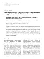
We consider a downlink scenario where the aim is to obtain
(transmitter) channel information at the base-station. The
considered situation is depicted in Figure 1. The picture
shows a base-station with m antennas and a mobile-station
with n antennas. Each transmitter and receiver chain is
characterized by an unknown gain and phase. The calibra-
tion coefficients are obtained using signals generated and
received locally at the base-station. The switches between
the receiver/transmitter pairs can be set independently.
The effective downlink channel, H
DL
(from base-station to
mobile-station), is given by
H
DL

= C
MS,rx
HC
BS,tx
,(1)
where C
MS,rx
and C
BS,tx
are diagonal and contain the complex
gain of the corresponding receiver(
=rx)/transmitter(=tx)
chain in the mobile-station(MS) or base-station(BS) along
the diagonal.
In the same way the effective uplink channel is given by
H
UL
= C
BS,rx
H
T
C
MS,tx
. (2)
In the following, we propose a technique to obtain a
matrix

H which has the same row-space as the true downlink
channel H
DL

. This information is sufficient for zero-forcing
techniques such as in this paper. We define the matrix

H as

H = H
UL,T
diag

1,
c
BS,tx
2
c
BS,rx
1
c
BS,tx
1
c
BS,rx
2
, ,
c
BS,tx
m
c
BS,rx
1
c

BS,tx
1
c
BS,rx
m

. (3)
We first need to show how the base-station obtains
the information needed to calculate

H. The uplink channel
matrix can obviously be obtained from the uplink signals.
Next, the elements of the diagonal matrix can be obtained
by the following calibration procedure. By sending a signal
from antenna no. 1 to antenna no. 2, the base-station obtains
c
BS,tx
1
c
BS,rx
2
c,wherec is the coupling between the antennas.
Likewise it may estimate the channel from antenna no. 2 to
EURASIP Journal on Advances in Signal Processing 3
c
BS,rx
1
c
BS,rx
1

c
BS,tx
m
c
BS,rx
m
SW
SW
.
.
.
H
SW
SW
.
.
.
c
MS,tx
1
c
MS,rx
1
c
MS,tx
n
c
MS,rx
n
Figure 1: Illustration of calibration procedure.

antenna no. 1 by transmitting in the opposite direction, thus
attaining an estimate of c
BS,tx
2
c
BS,rx
1
c. From these two estimates
the quotient c
BS,tx
2
c
BS,rx
1
/c
BS,tx
1
c
BS,rx
2
is obtained. By repeating
this procedure by transmitting signals between element no. 1
and all the other elements in the array (one at a time), all the
elements of the diagonal matrix in (3) can be obtained.
The next step is to obtain a relation between the true
downlink channel H
DL
and our estimate

H. This is done

through the derivations in (4)–(6)

H = C
MS,tx
HC
BS,rx
diag

1,
c
BS,tx
2
c
BS,rx
1
c
BS,tx
1
c
BS,rx
2
, ,
c
BS,tx
m
c
BS,rx
1
c
BS,tx

1
c
BS,rx
m

=
1
c
BS,tx
1
C
MS,tx
HC
BS,rx
×diag

c
BS,tx
1
,
c
BS,tx
2
c
BS,rx
1
c
BS,rx
2
, ,

c
BS,tx
m
c
BS,rx
1
c
BS,rx
m

=
c
BS,rx
1
c
BS,tx
1
C
MS,tx
H diag

1, c
BS,rx
2
, , c
BS,rx
m

×
diag


c
BS,tx
1
,
c
BS,tx
2
c
BS,rx
2
, ,
c
BS,tx
m
c
BS,rx
m

(4)
=
c
BS,rx
1
c
BS,tx
1
C
MS,tx
H diag


c
BS,tx
1
, c
BS,tx
2
, , c
BS,tx
m

(5)
=
c
BS,rx
1
c
BS,tx
1
C
MS,tx
HC
BS,tx
. (6)
The estimate (6) obviously differs from the true downlink
channel given by (1). Note that

H and H
DL
are related

through

H =
c
BS,rx
1
c
BS,tx
1
C
MS,tx

C
MS,rx

−1
H
DL
. (7)
When applying zero-forcing, knowing the row-space of

H is sufficient. It is evident from (7) that this information
may be obtained from

H. In cases other than zero-forcing,
using

H in place of the true channel matrix H
DL
is a subject

forfurtherstudy.
In a typical application, the calibration, that is, the
transmission between the antenna elements of the base-
station would be performed at the rate of change of the
gain and phase of the receiver and transmitter hardware.
Generally, such changes are attributed to temperature, and
thus the changes should be rather slow.
However, the channel coherence time, that is the variabil-
ity of the propagation channel H,ismuchfaster.Intypical
cellular and wireless LAN applications with Rayleigh fading
typical update times are on the order of milliseconds. Even
with those updates rates the channel can change substantially
between the time of channel estimation and use. A second
source of inaccuracy that should not be forgotten is thermal
noise.
A practical issue to consider regarding the selected
calibration scheme is that the transmission of the calibration
signal can cause interference somewhere else. However,
the signal can be made very weak. In fact a significant
requirement is that receiver chain is not saturated from an
overly strong signal. Another requirement is that the signal
actually passes all the way through the transmitter chain, the
transmitting antenna, the receiving antenna, and the receive
chain and does not leak through.
In the implementation herein we used a calibration signal
which was 30 dB weaker than the signals transmitted from
the mobile-station (we are here referring to the power at the
transmitter). This allowed us to use the same gain control
word setting at the receiver, during calibration as well as
during measurements. When this is not the case (i.e., variable

gain control word is used) the base-station would need to
4 EURASIP Journal on Advances in Signal Processing
Calibration
1
⇒ 2
Calibration
2 ⇒ 1
Uplink Downlink
6ms 6ms 6ms 6ms
Time
Figure 2: The multiframe in the USRP implementation.
create tables of the gain and phase of its receiver chains as a
function of the gain control word. The base-station would
then use these values to adjust the calibration coefficients
accordingly.
3. Implementation
Our implementation was done on the universal software
radio peripheral (USRP1). This platform consists of a moth-
erboard with a USB interface, an FGPA, a microcontroller,
and four 64 MHz ADC and 128 MHz DAC converters, [13].
The board interfaces to a range of transceiver daughter-
boards for various frequency bands (see us
.com/). We are using a pair of RFX1800 daughter-boards
on our USPRs. The USRP board is generally connected
to a Linux PC which is also the case herein. The GNU
Radio project (see />software framework and lots of signal processing modules.
In our implementation herein we are however only using
the functionality to receive and transmit buffers provided by
GNU Radio while all the signal processing is done in Matlab.
We have utilised two nodes, one base-station and one

mobile-station, and used emulation techniques to investigate
a system consisting of two base-stations and two mobile-
stations, as will be described in more detail below.
The node representing the base-station is employing two
antennas, and the mobile-station is using a single antenna.
We are using an OFDM modulation with a sample frequency
of 2 MHz. An FFT length of eight with a cyclic prefix length
of two samples is employed, resulting in a subcarrier spacing
of 250 kHz. Of the eight subcarriers the innermost five are
used while the remaining three are nulled. The modulation
scheme used is uncoded QPSK. The multiframe employed
is indicated in Figure 2. Three precoding schemes are used:
single-antenna, maximum ratio, and zero-forcing. In the
maximum ratio case the weights are given by
w
MR
= c

h
d
,(8)
where c is a scalar and

h
d
is the channel estimated from
the uplink (the channels in this section are defined as the
conjugate transpose of

H defined in Section 2). In the zero-

forcing case the transmit vector is selected as
w
ZF
= c
⎛
⎜
⎝
I −
1




h
i



2

h
i

h
∗
i
⎞
⎟
⎠
h

d
,(9)
where

h
i
is the channel estimate of the cochannel user seen at
the base-station. In the single antenna precoding case, which
is included as a reference only, one element of the precoding
vectorsissettozero.Allprecodershavethesamenorm.
The precoding should ideally be performed on a subcarrier
basis. However, our emulation strategy only allows one set of
weightsforallsubcarriersaswewillseebelow.
In the first frame calibration signals are sent internally
from antenna no. 1 to antenna no. 2, while in the second the
signal is sent in the opposite direction. The received signal is
used as described in Section 2 in order to estimate the TDD
calibration coefficient that is (c
tx
2
c
rx
1
)/(c
tx
1
c
rx
2
). The calibration

scheme is applied independently for each subcarrier using a
CW signal with the corresponding frequency.
The uplink and downlink frames in Figure 2 are identical,
except that the uplink frame is transmitted from the mobile-
station to the base-station and the downlink frame in the
opposite direction. The frames contain fourteen burst pairs.
The two bursts in a burst pair are identical except that the
first one is transmitted on antenna no. 1 and the other
on antenna no. 2. Each burst contains fourteen OFDM
symbols. There is a lot of space in all the 6 ms buffers. This
space could be eliminated, but our interest is to study the
principal limitations of TDD reciprocity-based precoding
and not to optimise the throughput of our test system. In
addition, the space is utilised in order to estimate the noise
level. The transmitted OFDM signals are pre-calculated in
Matlab, and the received signals are then stored on hard-
disc for postprocessing in Matlab. We are able to emulate the
performance of a TDD reciprocity-based system with two
base-stations and mobile-stations by combining multiple
measurements. The details of this emulation are given in
Appendix A. A key point in the emulation is the fact that
we have transmitted the same burst with both antennas. This
allows us to weight the contributions from the two antennas
of the base-station and sum them to construct the signal
that would have been received at the mobile-station given
a certain precoder. This relies on the assumption that the
receiver is linear, which appears to be a mild assumption.
In the emulation process, the uplink channels are
estimated by the base-station based from the uplink frame;
see Figure 2. The channel estimation is done independently

among the subcarriers by cross-correlation with the trans-
mitted signal. The base-station then applies the calibration
coefficient to obtain estimates of the downlink channels.
Given the downlink channel the base-station can calculate
the precoding weights. The signal received at the mobile-
station from the two base-stations is then calculated by
EURASIP Journal on Advances in Signal Processing 5
12 m
∗
Figure 3: Floor-plan layout. The asterix and square indicate the postion of the two base-stations. The mobile station moved in and out of
the offices between the two base-stations.
weighing the antenna signals according to the selected
weights. The mobile-station then demodulates the combined
signal assuming the first symbol to be known. More details
are provided in Appendix A.
4. Measurement Campaign
Themeasurementsweredoneoninanoffice environment.
The base-station was placed at the points marked with an
asterisk and a square (Figure 3). The mobile-station was
moving at some 5–10 cm/sec moving in and out of offices in
between the base-stations. The multiframes were separated
by some ten seconds to achieve fading decorrelation between
measurements. Some measurements close to the base-station
had to be removed because the receiver was saturated from
the strong signal and the absence of automatic gain control.
A total of 152 good multiframes were collected. These
measurements are divided into four parts: A, B, C, and D.
These parts represent the different paths in 152/4
= 38 two-
base-station two-mobile scenarios. This is described in more

detail in Appendix A.
Dual slant polarised patch antennas are used as trans-
mitter antennas and a single slant patch as receiver antenna.
The output power is
−6 dBm divided equally among the
five carriers with 250 kHz spacing. A higher output power
leads to bit errors due to nonlinearity in the power amplifiers
(varies between amplifier units). The carrier frequency is
1902.5 MHz.
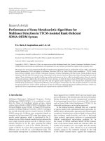
5. Measurement Results
The performance of single-antenna, maximum-ratio, and
zero-forcing pre-coding in a two-cell scenario is evaluated
based on measurements as described in Appendix A.The
mean bit error rate (uncoded) is 17.1%, 11.7%, and 0.9%, for
single-antenna, maximum-ratio, and zero-forcing, respec-
tively. The outage probability that is the probability of a
0
0.1
0.2
0.3
0.4
0.5
0.6
0.7
0.8
0.9
1
Pr {SNDR <x}
−30 −20 −10 0 10 20 30 40
(dB)

Single antenna
Maximum ratio
Zero-forcing
Figure 4: Cumulative distribution of SINDR at the receiver.
single bit error or more in a 6 ms frame is 74%, 39%,
and 14% for single-antenna, maximum-ratio, and zero-
forcing, respectively. The cumulative distribution function
of the obtained signal to interference, noise and distortion
measurements are shown in Figure 4. We note that the
zero-forcing outperforms single-antenna and maximum-
ratio transmission, where the difference between the latter
twotechniquesisrelativelyminor.Thesystemisclearly
interference limited as the signal to noise ratio was found to
be higher than 30 dB, 95% of the time.
5.1. Coordinated Multipoint Scenar io (CoMP). We no w
consider a coordinated multipoint (CoMP) scenario where
scheduling is performed jointly for the two cells. We further
6 EURASIP Journal on Advances in Signal Processing
0
0.1
0.2
0.3
0.4
0.5
0.6
0.7
0.8
0.9
1
Pr {capacity <x}

4 6 8 1012141618
bits/symbol
SU
MU
Optimal
Figure 5: Throughput of single-user and multiuser scheduling.
assume that adaptive modulation and coding are employed,
and that the sum of interference noise and distortion can
be modelled as Gaussian noise. Under these assumptions
we model the throughput of each channel use as log
2
(1 +
SNIDR) (a channel is here a certain subcarrier and a certain
OFDM symbol). Two users are considered as before. A joint
scheduler would in such a scenario select the best way of
sharing the channel, either a single-user at a time (SU) that
is, using time division or by simultaneous use by both users
(MU) (in the SU case we use maximum-ratio transmission
while we use zero-forcing in the MU case). However, as we
will see later in Section 6.3, predicting the SNIDR is difficult
which makes it difficult to realise these capacities in practise.
Here, however we assume the genie aided scenario where
the base-stations knows exactly the SNIDR. Thus for each
of the 38 measurements we select the solution that gives the
maximum sum capacity. In the SU case we of course multiply
the single-user capacity by a factor 0.5 to account for the
time division sharing of the channel. Figure 5 shows the
cumulative distribution of the optimum solution together
with the reference cases of TD-only and SU-only. In the
optimal mix, the MU-solution is chosen in 95% of the cases

which shows that zero-forcing is meaningful.
5.2. Ideal Case versus the Measurements. A natural question
is how far from ideal theory the measurement results herein
are. The ideal case represents the way most researchers would
simulate the system considered, namely, assuming perfect
channel knowledge at the base-stations and only thermal
noise and cochannel interference impairing the reception.
The performance of this case has been obtained for zero-
forcing and is labelled as “ideal” in Figure 7 (more details
are given in the next section). In contrast the curve labelled
“measurement” represents the results actually obtained from
the measurements. As is evident to the reader, the gap
0
0.1
0.2
0.3
0.4
0.5
0.6
0.7
0.8
0.9
1
Pr {error <x-axis}
00.05 0.10.15 0.20.25
Error
Measurement
Model
Figure 6: Measured channel prediction error.
between the two curves is substantial. This issue is analysed

further in the next section.
6. Analysis of Impairments
In this section we analyse the impact of radio frequency (RF)
impairments on the performance of the system.
6.1. Errors in the Channel Prediction. The “prediction” of the
downlink channel is obtained by calculating the calibration
factor (c
tx
2
c
rx
1
)/(c
tx
1
c
rx
2
) and applying it to the uplink channel
estimate according to (6). Based on our measurements we
can compare the error between the “predicted” downlink
channel estimate and the true channel estimate. In this
comparison we use the downlink channel estimated at the
mobile-station as the “true” downlink channel. We define the
error, e, between the “predicted” downlink channel

h and the
“true” downlink channel h
DL
as

e
=






1 −




h
∗
h
DL



2




h



2

h
DL

2
.
(10)
We note that this definition is invariant to any scaling
error. The error is also related to the performance of zero-
forcing precoding as described in Appendix B.InFigure 6
the cumulative distribution of the prediction error, e,is
plotted as the curve with legend “measurement.” It has been
verified that the influence of noise is negligible in these
measurements. Also plotted in Figure 6 is a “model” curve
which is the error, e, obtained from simulations using the
following error model:

h
model
= h
DL
+ e, (11)
EURASIP Journal on Advances in Signal Processing 7
0
0.1
0.2
0.3
0.4
0.5
0.6
0.7

0.8
0.9
1
Pr {SNIDR <x-axis}
−10 0 10 20 30 40 50 60 70
(dB)
Measurement
SNIDR k
dist
= 0.003
SINR k
dist
= 0
Ideal
Figure 7: Cumulative distribution of SNIDR at the receiver.
where e is a complex Gaussian random vector with indepen-
dent elements. The covariance matrix of e is given by
E

ee
∗

=
k
est
diag

h
DL
h

∗
DL

, (12)
where k
est
= 0.01. The plot shows fair agreement between the
model and the measurements. This does not fully prove the
model since the model is multidimensional while the error
measure is scalar. The intuition for the model is that errors
are multiplicative and thus proportional to the channel
amplitude.
6.2. Influence of Distortion. In Section 5 we presented the
performance of the system in terms of bit error rate (BER)
and signal to interference noise and distortion (SNIDR). In
order to investigate the contribution from distortion to the
SNIDR distribution of the zero-forcing solution, the SNIDR
obtained from the measurements is shown in Figure 7 as
the curve labelled “measurement.” Also shown in the figure
is a curve labelled “SINR, k
dist
= 0.” This curve was
obtained by using the exact same precoder weights as in the
“measurement” curve. However, we here calculate the signal
to noise and interference ratio (SINR), according to
SINR
=




w
∗
d
h
DL
d



2


w
∗
c
h
DL
c


2
+ σ
2
n
, (13)
where the subscripts “d” and “c” denote entities associated
with the desired and interfering (i.e. cochannel) base-station,
respectively. The noise level is based on measurements
during periods when there is no signal present. The channels
used in (13) are based on measurements from the data

at the mobile-station, while the weighting vectors were
based on the downlink channels predicted from the uplink
data. The gap between the “measurement” and “SINR,
k
dist
= 0” curve represents the influence of distortion.
In a typical simulation of our system one would assume
that the channel estimation is perfect (the noise level is
very small in our measurements). The performance of such
system is described by the curve “ideal” in Figure 7,where
we have used the channel matrices estimated in downlink
when calculating the pre-coding weights, when applying
(13). Thus the gap between the “measurement” and “ideal”
represents the total gap between theory and practise. In order
to bridge this gap we have presented an empirical model
for the channel prediction error in Section 6.1.However,
the distortion is also responsible for a great portion of the
gap between the “ideal” and “measurement” curves. Among
the major contributors of distortions in OFDM systems are
nonlinear amplifiers and phase-noise [10]. Previous studies
suggest that these can be modelled as Gaussian [10, 12, 14].
Thus with each transmitter or receiver branch we associate
a Gaussian noise to represent the distortion. We select the
power of this noise to be proportional to the transmitted
signal. Considering phase-noise this assumption can be
motivated from theory (see (16) of [10]), while for amplifier
nonlinearities it is only approximate. Thus the power of the
distortion noise in each receiver or transmitter branch is
assumed to be given by
σ

2
d
= k
dist
P, (14)
where the factor k
dist
can be interpreted as the error-vector-
magnitude [15]. We assume that the distortion noise is
independent between transmitter branches as was shown
by measurements in [12]andassumedin[11]. We fur-
ther assume that the distortion in the transmitter and
receiver chains are of equal power (i.e., the same k
dist
coefficient applies) since we are not able to separate them
in our measurements. Since the power of the signal at the
transmitter is given by the weights of the corresponding
antenna, the transmitter noise will be white with a covariance
matrix given by k
dist
diag(|w
1
|
2
, , |w
m
|
2
), where w
1

, , w
m
are the transmitter weights. This transmitter noise then
passes through the channel h
DL
. The power of transmitter
distortion is obtained by weighting the contribution of the
transmitter antennas with the channel gains and summing
the result. In compact form we can write this resulting noise
power as
w  h
DL

2
. The distortion noise of the receiver is
simply obtained by taking the power of the received signal
and multiplying by k
dist
. By applying these principles to our
case of two base-stations and a single mobile antenna we
obtain
SINDR
=



w
∗
d
h

DL
d



2


w
∗
c
h
DL
c


2
+ σ
2
tot
, (15)
where σ
2
tot
is given by
σ
2
tot
= σ
2

n
+ k
dist




w
d
h
DL
d



2
+



w
c
h
DL
c



2
+




w
∗
d
h
DL
d



2
+



w
∗
c
h
DL
c



2

.
(16)

8 EURASIP Journal on Advances in Signal Processing
−15
−10
−5
0
5
10
15
20
25
30
Actual SNIDR
−15 −10 −50 510152025
Predicted SNIDR
Figure 8: Prediction of the actual SNIDR. The x-axis is the
prediction and the y-axis the actually measured SNIDR.
Inordertoobtainavalueofk
dist
we first conducted a
series of measurements using a single transmitter antenna
measurement. Based on these measurements we set k
dist
=
0.003. The SNIDR calculated by using (15) is shown in
Figure 7. The curve is fairly close to the measurement results
up to the 80% level of the CDF.
6.3. Predicting the Performance. Inordertobeabletodo
CoMP as described in Section 5.1. we need to be able to
predict the downlink SNIDR, in order to do scheduling
and select the appropriate modulation and coding scheme.

In attempt to predict the downlink SNIDR we use (15).
However, now we use the predicted downlink channels
instead of the true downlink channels when evaluating (16)
since the base-station does not access to the true downlink
channel. The results are shown in Figure 8 where each
point represents a measurement result. The x-axis of the
point is the SNIDR predicted from (5) and the y-axis the
actual measured SNIDR. The prediction is relatively good in
average but the standard deviation of the prediction error is
3.5 dB. It is obvious that a better SNIDR prediction would
be much desired. Therefore, more research into this area is
needed.
7. Conclusions
In this paper we presented a method for TDD calibration
based on the reciprocity principle. The method is based on
transmitting and receiving signals between the elements of
the antenna array. The method does not require interactions
with other nodes or additional calibration circuitry. How to
use the method in a MIMO context is also indicated. We
further describe an implementation of maximum-ratio and
zero-forcing precoding on a wireless testbed called USRP
(see We study the performance in
terms of bit-error rate (BER) signal to noise, interference,
and distortion ratio (SNIDR) and throughput. The use of
zero-forcing precoder is shown to outperform maximum
ratio transmission.
We also analyse the error in the downlink channel
prediction by comparing the predicted channel vectors with
those actually obtained at the mobile station. A model for
the prediction error based on the measurements is proposed.

The impact of distortion is also factored out from the
measurements. We show that a simple error vector model
provides a reasonable model for the errors in an average
sense.
However, when we try to predict the SNIDR such
as required in a coordinated multipoint scenario (CoMP)
with joint scheduling, the prediction error is substantial
(standard deviation 3.7 dB). This shows that there is room
for substantial improvement in this respect.
Appendices
A. Details of the Implementation on USRP
A system with a single base-station and mobile-station can
be emulated as follows.
(1) Calculate the calibration constant (c
tx
2
c
rx
1
)/(c
tx
1
c
rx
2
)
from the calibration data stored at the base-station.
(2) Estimate the uplink channel based on the data stored
at the base-station.
(3) Predict the downlink channel using the uplink data

and the estimated calibration data.
(4) Calculate the precoder based on the obtained channel
knowledge.
(5) Construct the signal received by the mobile-station
by adding and weighting the two parts of the burst
pairs using the previously obtained weights.
(6) Demodulate the received signal assuming that the
first OFDM symbol of the burst is known.
(7) Estimate the SINDR by calculating the mean square
error between the sample-points and the true constel-
lation points.
There is one problem with the enumeration above. In
an OFDM system we would ideally transmit with different
precoder weights on different subcarriers. However, the
above emulation scheme does not allow that. On the other
hand, in our indoor propagation scenario the channel can be
regarded as flat over the five subcarriers spanning 1.25 MHz,
and thus the loss is negligible. Note, however, that we are
still able to study the channel estimation error on all the
subcarriers.
In order to develop the emulation scheme above for a case
with two base- and mobile-stations we need to elaborate the
procedure further. In order to do so, we need first to describe
the USRP measurement campaign in detail. The campaign
wasdoneinanoffice floor at a speed of 5–10 cm/sec with
ten seconds between multiframes to decorrelation in the fast
fading. The USRP measurement campaign consists of four
parts, campaign A, B, C, and D. In campaign A and B the
EURASIP Journal on Advances in Signal Processing 9
base-station was positioned at the asterisk of Figure 3 while

it was positioned at the square in campaign C and D. The
mobile-station was typically in the corridor and office rooms
close to the base-station marked by an asterisk in campaign
A and D, while it was close to the base-station marked by
a square in campaign B and C. In each subcampaign 38
measurements were made. We use the data measured in
campaign A and D to represent the channel between user
no. 1 and base-station no. 1 and no. 2, respectively, while the
data measured in campaign B and C represents the channel
between mobile-station no. 2 and base-station no. 1 and
no. 2, respectively. The performance of a two base-station
two mobile-station is then done by repeating the following
procedure for the 38 measured quartets of multiframes.
(1) Calculate the calibration constant (c
tx
2
c
rx
1
)/(c
tx
1
c
rx
2
)for
base-station no. 1 using data from campaign A and
D.
(2) Do likewise for base-station no. 2.
(3) Estimate the uplink channels between base-station

no. 1 and mobile-station no. 1 using calibration and
uplink data from campaign A.
(4) Estimate the uplink channels between base-station
no. 1 and mobile-station no. 2 using calibration and
uplink data from campaign D.
(5) Do likewise for base-station no. 2 using data from
campaign B and C.
(6) Calculate the precoders for base-station no. 1 and no.
2.
(7) Construct the signal received at mobile-station no. 1
by adding the contribution from base-station no. 1
and no. 2 using data from campaign A and D. The
contribution from base-station no. 1 is the sum of the
two transmitter antennas weighted by the precoder of
that base-station and likewise for base-station no. 2.
The signal from base-station no. 2 is offset one burst
pair so that the interfering signal carries a different
information content than the desired signal.
(8) Demodulate the signal received at mobile-station
no. 1. The first OFDM symbol of the desired base-
station is assumed known. The interference (i.e., the
contribution from the other base-station) is removed
from the training OFDM symbol.
(9) Estimate the SINDR by calculating the mean square
error between the sample-points and the true constel-
lation points.
(10) Repeat step (5)–(7) for mobile-station no. 2 with
obvious changes.
Note that we remove the interference from the channel
estimation, and no interference is added to the uplink

measurements.
During the measurements the nodes were synchronised
using a cable. The cable is connected to a general purpose
pin on each of the USRPs. The two nodes are polling the
pin continuously. When the pin changes polarity a frame
is started. The cable is driven by a square-wave generator
with half-period of 6 ms. Due to latencies in the USRP, USB,
and PCs the useful signal appears 1-2 ms into the received
buffer. The latency varies from frame to frame. Each frame
starts with a synchronisation sequence of 100 samples. When
the data is processed the timing of the received burst is
obtained by cross-correlating the received signal with the
known synchronisation sequence. This correlation is done
with several frequency offsets to simultaneously obtain the
frequency offset.
B. The Chosen Error Measure
Let us divide the true downlink channel h
DL
into two parts,
one which is aligned with the channel estimate,

h,andone
which is orthogonal to this channel estimate, that is,
h
DL
= P

h
h
DL

+ P
⊥

h
h
DL
=

h
∗
h
DL




h



2

h + e.
(B.1)
The“power”oftheerrorvectorisgivenby
e
2
= h
∗
DL

P
⊥

h
h
DL
=h
DL

2
−



h
∗
DL

h



2




h




2
.
(B.2)
If the channel estimate

h is that of a cochannel user, a
zero-forcing precoder would choose a weighting such that
w
∗
ZF

h = 0. The remaining interference is then given by
|w
∗
ZF
e|
2
, where the power of e is given by (B.2). The power
of
e needstobesetinrelationtoh
DL
. We therefore chose to
divide the power of
e by the power of h
DL
thus obtaining
e
2
h

DL

2
= 1 −



h
∗
DL

h



2




h



2
h
DL

2
= e

2
,
(B.3)
that is, the square of our chosen error measure e.
Acknowledgments
The research leading to these results has received funding
from the European Research Council under the European
Community’s Seventh Framework Programme (FP7/2007–
2013)/ERC Grant agreement no. 228044. The work has also
been performed partly within the framework of the Euro-
pean Commission funded IST-2002-2.3.4.1 COOPCOM
project.
10 EURASIP Journal on Advances in Signal Processing
References
[1] M. Bengtsson and B. Ottersten, “Optimal and suboptimal
transmit beamforming,” in Handbook of Antennas in Wireless
Communications, L. C. Godara, Ed., CRC Press, 2001.
[2] D.P.Palomar,J.M.Cioffi, and M. A. Lagunas, “Joint Tx-Rx
beamforming design for multicarrier MIMO channels: a uni-
fied framework for convex optimization,” IEEE Transactions on
Signal Processing, vol. 51, no. 9, pp. 2381–2401, 2003.
[3]Q.H.Spencer,A.L.Swindlehurst,andM.Haardt,“Zero-
forcing methods for downlink spatial multiplexing in mul-
tiuser MIMO channels,” IEEE Transactions on Signal Process-
ing, vol. 52, no. 2, pp. 461–471, 2004.
[4] S. Ramo, J. R. Whinnery, and T. Van Duzer, Fields and Waves
in Communication Electronics, John Wiley & Sons, New York,
NY, USA, 3rd edition, 1993.
[5] J. H. Winters, “Optimum combining in digital mobile radio
with cochannel interference,” IEEE Transactions on Vehicular

Technology, vol. 33, no. 3, pp. 144–155, 1984.
[6] S. Gollakota, S. D. Perli, and D. Katabi, “Interference align-
ment and cancellation,” in Proceedings of the ACM Conference
on Data Communication (SIGCOMM ’09), pp. 159–170,
August 2009.
[7] J C. Guey and L. D. Larsson, “Modeling and evaluation of
MIMO systems exploiting channel reciprocity in TDD mode,”
in Proceedings of the IEEE Vehicular Technology Conference, vol.
6, pp. 4265–4269, September 2004.
[8] M. Guillaud, D. T. M. Slock, and R. Knopp, “A prac-
tical method for wireless channel reciprocity exploitation
through relative calibration,” in Proceedings of the 8th Inter-
national Symposium on Signal Processing and Its Applications
(ISSPA ’05), pp. 403–406, August 2005.
[9] K. Nishimori, K. Cho, Y. Takatori, and T. Hori, “Automatic
calibration method using transmitting signals of an adaptive
array for TDD systems,” IEEE Transactions on Vehicular
Technology, vol. 50, no. 6, pp. 1636–1640, 2001.
[10] R. Corvaja, E. Costa, and S. Pupolin, “Analysis of M-QAM-
OFDM transmission system performance in the presence of
phase noise and nonlinear amplifiers,” in Proceedings of the
28thEuropeanMicrowaveConference, vol. 1, pp. 481–486,
October 1998.
[11] B. G
¨
oransson, S. Grant, E. Larsson, and Z. Feng, “Effect of
transmitter and receiver impairments on the performance of
MIMO in HSDPA,” in Proceedings of the 9th IEEE Workshop
on Signal Processing Advanced in Wireless Communications,pp.
496–500, 2008.

[12] C. Studer, M. Wenk, and A. Burg, “MIMO transmission
with residual transmit-RF impairments,” in Proceedings of the
International ITG Workshop on Smart Antennas (WSA ’10),pp.
189–196, February 2010.
[13] E. Blossom, “GNU Radio: tools for exploring the radio
frequency spectrum,” Linux Journal, vol. 2004, no. 122, 2004.
[14] D. Dardari, V. Tralli, and A. Vaccari, “A theoretical characteri-
zation of nonlinear distortion effects in ofdm systems,” IEEE
Transactions on Communications, vol. 48, no. 10, pp. 1755–
1764, 2000.
[15] R. A. Shafik, M. S. Rahman, A. H. M. R. Islam, and N. S.
Ashraf, “On the error vector magnitude as a performance met-
ric and comparative analysis,” in Proceedings of the IEEE-ICET
International Conference on Emerging Technologies ,Pershawar,
Pakistan, November 2006.