Climate Change and Variability Part 12 ppt

Simulated potato crop yield as an indicator of climate variability and changes in Estonia 373
GCM experiment and constructing a composite pattern for future climate change was first
introduced by Santer et al. (1990); later Hulme et al. (2000) reported the clear supremacy of
the technique over just only one model. The data are displayed in MAGICC/SCENGEN in a
grid resolution of 2.5º latitude/longitude, thus the Estonian territory is covered by three
grid boxes, with medium coordinates 58.8ºN/21.3ºE, 58.8ºN/23.8ºE and 58.8ºN/26.3ºE.
Kuressaare and Tartu fall into two outermost boxes. However, the direct use of the
SCENGEN output is not possible, because these predictions are available as changes in
monthly means, but the crop model depends on daily time-series of weather as one of its
main inputs. To calculate the future values of MPY, we used observed daily weather data in
those stations during the baseline period 1965-2006. This shorter period is applied instead of
previously used longer periods, since in climate change calculations it is necessary to use
data outside the heretofore growing period. Global radiation was assumed not to change.
Future daily temperatures and precipitation were calculated by adding the predicted
monthly corrections to the observed series of daily data. This way, not just the one average
predicted future value for temperature and precipitation, but 41 possible series of those
meteorological elements were obtained for the two target years, suggesting the possible
future weather distribution. Such setup also leads to the variability in the future climates
being almost identical to the variability of the historical climate. Although the variability of
climate in the future may alter (Rind et al., 1989; Mearns, 2000), inducing possible decrease
in mean crop yields (Semenov & Porter, 1995; Semenov et al., 1996), some researchers
(Barrow et al., 2000; Wolf, 2002) have reported that for potato, changes in climatic variability
in northern Europe generally resulted in no changes in mean yields and its coefficient of
variation.
Thus converted future weather data series are employed to calculate the date and the value
of the initial water storage in the soil (or the date when the soil moisture falls below the field
capacity), the date of the permanent increase in temperature to above 8 °C in the spring, the
dates of the last and first night frosts (≤ -2 °C), and the date of the permanent drop in
temperature to below 7 °C in autumn for each individual year of the new series. For
determination of the soil water status in spring a relationship between radiation balance R

fc

from permanent transition of temperature over 0º C to soil moisture fall below the field
capacity, and meteorological data was derived using 30-year data of 13 stations of the
Estonian Agrometeorological Network. To calculate R
fc
, incoming global radiation and
evaporative energy of precipitation (precipitation multiplied by latent evaporative heat)
were accounted. The strongest correlations of R
fc
were achieved with temperature sums
from March to April T
3-4
and precipitation sums from February to April U
2-4
:

R
fc
= 468.2 – 1.587 T
3-4
– 0.517 U
2-4
r = 0.66 (1)

To apply relationship (1) into the future dataset, a submodel calculates R
fc
as well as
permanent date of temperature rise over 0º C for each year of the new weather data series
for 2050 and 2100. Next, from that date, the running radiation balance is summarized day-

by-day. The date when the running radiation balance exceeds R
fc
is counted as the date of
achieving the soil field capacity and it is considered as the ‘first possible’ planting date.
Additionally, ‘optimal planting date’ is applied – the date achieved by postponing the day
of planting in model calculations day-by-day until the maximum yield is obtained. To
prevent staying to a side maximum this postponing is conducted until the MPY drops below
70% of its maximum value, or until the date of summer equinox.
The dates of last and first night frosts in the future series are found on the basis of the earlier
determined relationships between mean daily air temperature and ground level minimum
temperature, dependent on the radiation sum of previous day.

3. Results
3.1 Time series of meteorological resources: current climate
Series of meteorologically possible yield were compiled for early and late maturing potato
varieties in two different Estonian localities. In Table 1 we present long-term mean yields
calculated with existing meteorological data series, using real and computed (both first
possible and optimal) planting dates; the yields thus describe real, possible and optimal
climatic resources for plant growth during given period.
With real planting dates, there was practically no difference in average values of the MPY
between long and short (from 1965) series. As expected, the late variety produced higher
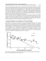
yields at all locations. Overall, the MPY series showed only weak and insignificant trends
(Fig. 5), although reliable trends are apparent for some shorter periods. The longest period
with a significant (P < 0.05) decreasing trend was observed in Kuressaare from 1977 to 2006.
Generally, ‘Anti' demonstrated higher variance in yields. For both varieties, the variability
reached higher in Kuressaare. Variability increases in all cases when using computed
planting dates instead of real dates.
Closer investigation of the MPY variability showed a significant increase in variance in
Tartu since the early 1980s. In the MPY calculations contrived with real meteorological data,
the standard deviation of MPY was significantly lower for ‘Maret’ in 1901-1980 compared to

1981-2006 (P = 0.006, according to F test); for ‘Anti’, the change was smaller yet significant (P
= 0.046). When using shorter time series and optimal planting times, the same difference in
yield variance was detected both for ‘Maret’ (P = 0.002) and ‘Anti’ (P = 0.015). The
meteorological elements series revealed no similar changes in climate variability. Reliable
dispersion differences were detected only in the precipitation series, but their significance
was lower than that of the yields.

ANTI MARET
Tartu Kuressaare Tartu Kuressaare
MPY Var.
coeff.
MPY Var.
coeff.
MPY Var.
coeff.
MPY Var.
coeff.
Real dates
Long series to 2006 55.5 0.20 50.3 0.27 45.0 0.16 37.8 0.21
1965-2006 54.5 0.21 50.3 0.28 45.1 0.19 37.7 0.22
1901-1980 56.1 0.18 45.5 0.14
1981-2006 53.9 0.25 43.5 0.22
1923-1938 51.0 0.16
1939-2006 50.1 0.29
Computed dates
1965-2006, first
planting date
58.8 0.24 49.8 0.33 42.4 0.18 38.2 0.27
1965-2006, optimum
planting date

58.9 0.23 50.2 0.32 44.0 0.19 39.3 0.26
Table 1. Mean values of MPY and corresponding coefficient of variation for different
periods.
Climate Change and Variability374
Therefore, the separate meteorological elements did not reflect the influence of their
combined effect on the variability of biological production. Significant differences in yield
variability, not identified in the meteorological series, were also observed for ‘Anti’ at
Kuressaare, where the standard deviation was approximately two times lower before 1939
than in later periods (P < 0.017).

Tartu Maret
y = -0,16x + 368,4
r = -0.24; p=0.1
y = 0,007x + 31,3
r = 0,03; p=0.8
15
40
65
1965-2006, optimal planting
Long series to 2006, real planting
Tartu Anti
y = -0,02x + 102,5
r = -0,07; p=0.5
y = 0,009x + 41,9
r = 0.01; p=0.9
15
40
65
Kuressaare Maret
y = -0,09x + 209,3

r = -0,1; p=0.5
y = -0,004x + 44,7
r = -0,01; p=0.9
15
40
65
Kuressaare Anti
y = -0,02x + 83
r = -0,03; p=0.8
y = 0,03x - 9,4
r = 0,02; p=0.9
15
40
65
1900 1910 1920 1930 1940 1950 1960 1970 1980 1990 2000
Year

Fig. 5. Series of MPY of the early potato variety ‘Maret’ and the late potato variety ‘Anti’ in
Tallinn and Kuressaare.
3.2 Relationships between MPY and other indicators
In Estonia, like elsewhere in temperate zone, crop yield variation is highly influenced by
weather conditions (Carter, 1996; Karing et al.,1999). When using real, measured potato
yield data, potato yield variance was found to be mostly dependent on weather conditions,
while the impact of fertilization and soil management proved less significant and in
interaction with weather (Saue et al., 2010). Of meteorological conditions, potato proved
the most susceptible to spring temperatures, yielding higher in years with a warm spring;
negative linear relation between yields and precipitation during the same period concurred.
The positive influence of precipitation was expressed after flowering.
In this paragraph, we will compare simulated yields and direct meteorological series of
precipitation, temperature and solar radiation, using accumulated values for those

meteorological elements over different periods, in order to explain the extent to which
individual factors allow us to describe the whole complex. Correlation analyses (linear and
second-order polynomial) were performed.
In Tartu , linear correlations between MPY and the accumulated meteorological factors were
weak, although they were significant in some cases since the series were long (Table 2). The
correlations with temperature were slightly higher, but only for the early variety.
In Kuressaare, significant (P < 0.01) linear correlations were identified between MPY and all
the accumulated meteorological factors in the selected periods: positive for precipitation and
negative for solar radiation and temperature. In general, the period with the highest
correlations began earlier for precipitation (from May for ‘Maret’ and from June for ‘Anti’),
and later for temperature and radiation (from June and July, respectively). The results for
Kuressaare are quite different from those for Tartu because its location on the island of
Saaremaa in the western part of Estonia is characterised by a mild marine climate and dry
summers. Low precipitation at the beginning of summer causes dry conditions, so water
deficit is the main limiting factor there. The relationships between MPY and solar radiation
and temperatures are largely indirect, and these factors correlate negatively with
precipitation.
As a rule, if a curve with a maximum describable by a second-order polynomial is applied,
better correlation will be apparent between MPY and the accumulated meteorological
elements. This means that for all factors, the limitation derives from both deficit and excess.
Again, the highest correlations occurred in Kuressaare: for ‘Anti’ with precipitation (June-
August: r = -0.77, May-August: r = -0.76), and for ‘Maret’ with temperature from June to
September (r = -0.71). The only exception, where the correlations are almost equal on the
linear and polynomial curves, is the early variety in Kuressaare. There, the conditions are
dry, especially in the first half of summer, so the limiting factor for the early variety in most
years is a deficit of precipitation. For the late variety, the decrease in yield is occasionally
caused by an excess of water. However, the latter is much more common in inland regions,
represented by Tartu, where intense rainy periods produce soil moisture near its maximum
content in June and July, causing the loss of soil aeration and a very significant reduction in
yield.

The limiting from two sides and high variances between MPY and the cumulative
meteorological elements allow us to conclude that, under our conditions, MPY gives
qualitatively new information about climate variability in summer, especially regarding
climatic favourableness, by integrating the effects of different weather factors. In conditions
with one very dominant limiting factor, there is no need for such an indicator, e.g., near the
Simulated potato crop yield as an indicator of climate variability and changes in Estonia 375
Therefore, the separate meteorological elements did not reflect the influence of their
combined effect on the variability of biological production. Significant differences in yield
variability, not identified in the meteorological series, were also observed for ‘Anti’ at
Kuressaare, where the standard deviation was approximately two times lower before 1939
than in later periods (P < 0.017).

Tartu Maret
y = -0,16x + 368,4
r = -0.24; p=0.1
y = 0,007x + 31,3
r = 0,03; p=0.8
15
40
65
1965-2006, optimal planting
Long series to 2006, real planting
Tartu Anti
y = -0,02x + 102,5
r = -0,07; p=0.5
y = 0,009x + 41,9
r = 0.01; p=0.9
15
40
65

Kuressaare Maret
y = -0,09x + 209,3
r = -0,1; p=0.5
y = -0,004x + 44,7
r = -0,01; p=0.9
15
40
65
Kuressaare Anti
y = -0,02x + 83
r = -0,03; p=0.8
y = 0,03x - 9,4
r = 0,02; p=0.9
15
40
65
1900 1910 1920 1930 1940 1950 1960 1970 1980 1990 2000
Year

Fig. 5. Series of MPY of the early potato variety ‘Maret’ and the late potato variety ‘Anti’ in
Tallinn and Kuressaare.
3.2 Relationships between MPY and other indicators
In Estonia, like elsewhere in temperate zone, crop yield variation is highly influenced by
weather conditions (Carter, 1996; Karing et al.,1999). When using real, measured potato
yield data, potato yield variance was found to be mostly dependent on weather conditions,
while the impact of fertilization and soil management proved less significant and in
interaction with weather (Saue et al., 2010). Of meteorological conditions, potato proved
the most susceptible to spring temperatures, yielding higher in years with a warm spring;
negative linear relation between yields and precipitation during the same period concurred.
The positive influence of precipitation was expressed after flowering.

In this paragraph, we will compare simulated yields and direct meteorological series of
precipitation, temperature and solar radiation, using accumulated values for those
meteorological elements over different periods, in order to explain the extent to which
individual factors allow us to describe the whole complex. Correlation analyses (linear and
second-order polynomial) were performed.
In Tartu , linear correlations between MPY and the accumulated meteorological factors were
weak, although they were significant in some cases since the series were long (Table 2). The
correlations with temperature were slightly higher, but only for the early variety.
In Kuressaare, significant (P < 0.01) linear correlations were identified between MPY and all
the accumulated meteorological factors in the selected periods: positive for precipitation and
negative for solar radiation and temperature. In general, the period with the highest
correlations began earlier for precipitation (from May for ‘Maret’ and from June for ‘Anti’),
and later for temperature and radiation (from June and July, respectively). The results for
Kuressaare are quite different from those for Tartu because its location on the island of
Saaremaa in the western part of Estonia is characterised by a mild marine climate and dry
summers. Low precipitation at the beginning of summer causes dry conditions, so water
deficit is the main limiting factor there. The relationships between MPY and solar radiation
and temperatures are largely indirect, and these factors correlate negatively with
precipitation.
As a rule, if a curve with a maximum describable by a second-order polynomial is applied,
better correlation will be apparent between MPY and the accumulated meteorological
elements. This means that for all factors, the limitation derives from both deficit and excess.
Again, the highest correlations occurred in Kuressaare: for ‘Anti’ with precipitation (June-
August: r = -0.77, May-August: r = -0.76), and for ‘Maret’ with temperature from June to
September (r = -0.71). The only exception, where the correlations are almost equal on the
linear and polynomial curves, is the early variety in Kuressaare. There, the conditions are
dry, especially in the first half of summer, so the limiting factor for the early variety in most
years is a deficit of precipitation. For the late variety, the decrease in yield is occasionally
caused by an excess of water. However, the latter is much more common in inland regions,
represented by Tartu, where intense rainy periods produce soil moisture near its maximum

content in June and July, causing the loss of soil aeration and a very significant reduction in
yield.
The limiting from two sides and high variances between MPY and the cumulative
meteorological elements allow us to conclude that, under our conditions, MPY gives
qualitatively new information about climate variability in summer, especially regarding
climatic favourableness, by integrating the effects of different weather factors. In conditions
with one very dominant limiting factor, there is no need for such an indicator, e.g., near the
Climate Change and Variability376
Polar Circle, where MPY correlates very well with temperature (Sepp et al., 1989) or in arid
regions, where the dominant factor is water deficit. For the stations analyzed in our work,
Kuressaare is the most likely to be affected by a single dominant limiting factor, but the
variance is still quite high there.

Station
Meteo-
element
Relation
-ship
Early variety 'Maret' 'Late variety Anti'
May-Aug June-Aug May-Sept May-Aug June-Aug May-Sept
Tartu

R LIN 0,03 0,02 0.03 0,01 -0,03 0.02
POL
0,36 0,41 0.31 0,47 0,52 0.43
P LIN 0,07 0,02 0.13 0,06 0,12 0.03
POL
0,53 0,40 0.49 0,64 0,56 0.40
T LIN
0,26 0,37

0.24 0,04 0,20 0.03
POL
0,35 0,50
0.29
0,41 0,55 0.35
POL 0,25
0,32 0.26 0,34 0,35 0.34
P LIN 0,19
0,27
0.05
0,26 0,34
0.10
POL
0,31 0,33 0.34 0,42 0,46 0.42
T LIN 0,17
0,41
0.24 0,14 0,09 0.08
POL
0,41 0,52 0.34 0,46 0,44 0.41
Kuressaare
R

LIN
0,50 0,55 0.51 0,46 0,56 0.45
POL
0,50 0,55 0.51 0,47 0,57 0.47
P

LIN
0,65 0,61 0.64 0,65 0,72 0.61

POL
0,68 0,66 -0.65 0,76 0,77 0.69
T

LIN
0,56 0,68 0.61 0,30 0,44 0.35
POL
0,58 0,69 0.62 0,48 0,57 0.51
Table 2. Correlation coefficients r for the linear (LIN) and polynomial (POL) relationships
between meteorologically possible yield (MPY) and accumulated solar radiation (R),
precipitation (P), and temperature (T) at two stations. Bold indicates significance levels of P
< 0.01.

3.3 Climate Change
Most climate change scenarios project that greenhouse gas concentrations will increase
through 2100 with a continued increase in average global temperatures (IPCC, 2007). Results
of the four emission scenarios, each containing 18 General Circulation Models (GCM)
experiments used in SCENGEN provide a wide variety of possible climate change scenarios
(Table 3). In this paragraph we will look at the results by four illustrative emission scenarios,
achieved by using the multi-model average for two locations in Estonia. All scenarios
project the increase in annual mean temperature, the highest warming is supposed to take
place during the cold part of the year (Fig. 6). During the plant-growth period (April to
September), the increase of air temperature will be lower. Average annual precipitation is
also predicted to increase (Fig. 7), however, changes in the annual range of monthly
precipitation vary highly between models and scenarios and are less certain than changes in
temperature. On average, the highest change in precipitation is predicted for January and
November; August and September are predicted a small increase or even a slight decrease.
All the projected climatic tendencies have already been noted during the last century
(Jaagus, 2006), indicating evident climate warming in Estonia. In previous analogous works
(Keevallik, 1998; Karing et al., 1999; Kont et al., 2003), temperature rise has been predicted

higher; however we believe that moderate warming is more realistic.

Year
Scenario
Temperature
change, º C
Precipitation change,
%
Tartu
Kures-
saare
Tartu
Kures-
saare
2050
A1B 2.40 2.37 8.5 8.1
A2 2.60 2.54 10.0 8.8
B1 1.73 1.71 6.2 5.8
B2 2.25 2.24 8.1 8.0
2100
A1B 4.65 4.64 16.2 16.3
A2 5.78 5.72 20.7 19.5
B1 3.11 3.14 10.7 11.2
B2 4.13 4.13 14.7 14.4
Table 3. Changes in annual air temperature and precipitation calculated as a mean of
experiments by 18 different GCM for four different emission scenarios.

Tartu 2100 A2
1
2

3
4
5
6
7
8
9
10
11
12
Year
-10
0
10
20
Temperature change,
C

Tartu 2100 B1
1
2
3
4
5
6
7
8
9
10
11

12
Year
-10
0
10
20

Kuressaare 2100 A2
1
2
3
4
5
6
7
8
9
10
11
12
Year
-10
0
10
20
Temperature change,
C

Kuressaare 2100 B1
1

2
3
4
5
6
7
8
9
10
11
12
Year
-10
0
10
20

Fig. 6. Changes in monthly mean temperature (º C) predicted by 18 global climate models
for the A2 and B1 emissions scenarios for year 2100 compared to the baseline period (1961–
1990) at two Estonian sites. Lines connect the values of monthly mean change, boxes mark
mean change ± standard deviation and whiskers mark the range of all models.
Simulated potato crop yield as an indicator of climate variability and changes in Estonia 377
Polar Circle, where MPY correlates very well with temperature (Sepp et al., 1989) or in arid
regions, where the dominant factor is water deficit. For the stations analyzed in our work,
Kuressaare is the most likely to be affected by a single dominant limiting factor, but the
variance is still quite high there.

Station
Meteo-
element

Relation
-ship
Early variety 'Maret' 'Late variety Anti'
May-Aug June-Aug May-Sept

May-Aug

June-Aug

May-Sept
Tartu

R LIN 0,03 0,02 0.03 0,01 -0,03 0.02
POL
0,36 0,41 0.31 0,47 0,52 0.43
P LIN 0,07 0,02 0.13 0,06 0,12 0.03
POL
0,53 0,40 0.49 0,64 0,56 0.40
T LIN
0,26 0,37
0.24 0,04 0,20 0.03
POL
0,35 0,50
0.29
0,41 0,55 0.35
POL 0,25
0,32 0.26 0,34 0,35 0.34
P LIN 0,19
0,27
0.05

0,26 0,34
0.10
POL
0,31 0,33 0.34 0,42 0,46 0.42
T LIN 0,17
0,41
0.24 0,14 0,09 0.08
POL
0,41 0,52 0.34 0,46 0,44 0.41
Kuressaare
R

LIN
0,50 0,55 0.51 0,46 0,56 0.45
POL
0,50 0,55 0.51 0,47 0,57 0.47
P

LIN
0,65 0,61 0.64 0,65 0,72 0.61
POL
0,68 0,66 -0.65 0,76 0,77 0.69
T

LIN
0,56 0,68 0.61 0,30 0,44 0.35
POL
0,58 0,69 0.62 0,48 0,57 0.51
Table 2. Correlation coefficients r for the linear (LIN) and polynomial (POL) relationships
between meteorologically possible yield (MPY) and accumulated solar radiation (R),

precipitation (P), and temperature (T) at two stations. Bold indicates significance levels of P
< 0.01.

3.3 Climate Change
Most climate change scenarios project that greenhouse gas concentrations will increase
through 2100 with a continued increase in average global temperatures (IPCC, 2007). Results
of the four emission scenarios, each containing 18 General Circulation Models (GCM)
experiments used in SCENGEN provide a wide variety of possible climate change scenarios
(Table 3). In this paragraph we will look at the results by four illustrative emission scenarios,
achieved by using the multi-model average for two locations in Estonia. All scenarios
project the increase in annual mean temperature, the highest warming is supposed to take
place during the cold part of the year (Fig. 6). During the plant-growth period (April to
September), the increase of air temperature will be lower. Average annual precipitation is
also predicted to increase (Fig. 7), however, changes in the annual range of monthly
precipitation vary highly between models and scenarios and are less certain than changes in
temperature. On average, the highest change in precipitation is predicted for January and
November; August and September are predicted a small increase or even a slight decrease.
All the projected climatic tendencies have already been noted during the last century
(Jaagus, 2006), indicating evident climate warming in Estonia. In previous analogous works
(Keevallik, 1998; Karing et al., 1999; Kont et al., 2003), temperature rise has been predicted
higher; however we believe that moderate warming is more realistic.

Year
Scenario
Temperature
change, º C
Precipitation change,
%
Tartu
Kures-

saare
Tartu
Kures-
saare
2050
A1B 2.40 2.37 8.5 8.1
A2 2.60 2.54 10.0 8.8
B1 1.73 1.71 6.2 5.8
B2 2.25 2.24 8.1 8.0
2100
A1B 4.65 4.64 16.2 16.3
A2 5.78 5.72 20.7 19.5
B1 3.11 3.14 10.7 11.2
B2 4.13 4.13 14.7 14.4
Table 3. Changes in annual air temperature and precipitation calculated as a mean of
experiments by 18 different GCM for four different emission scenarios.

Tartu 2100 A2
1
2
3
4
5
6
7
8
9
10
11
12

Year
-10
0
10
20
Temperature change,
C

Tartu 2100 B1
1
2
3
4
5
6
7
8
9
10
11
12
Year
-10
0
10
20

Kuressaare 2100 A2
1
2

3
4
5
6
7
8
9
10
11
12
Year
-10
0
10
20
Temperature change,
C

Kuressaare 2100 B1
1
2
3
4
5
6
7
8
9
10
11

12
Year
-10
0
10
20

Fig. 6. Changes in monthly mean temperature (º C) predicted by 18 global climate models
for the A2 and B1 emissions scenarios for year 2100 compared to the baseline period (1961–
1990) at two Estonian sites. Lines connect the values of monthly mean change, boxes mark
mean change ± standard deviation and whiskers mark the range of all models.
Climate Change and Variability378
Tartu 2100 A2
1
2
3
4
5
6
7
8
9
10
11
12
Year
-200
-100
0
100

200
Precipitation change,
%

Tartu 2100 B1
1
2
3
4
5
6
7
8
9
10
11
12
Year
-200
-100
0
100
200

Kuresaare 2100 A2
1
2
3
4
5

6
7
8
9
10
11
12
Year
-200
-100
0
100
200
Precipitation change,
%

Kuressaare 2100 B1
1
2
3
4
5
6
7
8
9
10
11
12
Year

-200
-100
0
100
200

Fig. 7. Changes in monthly sum of precipitation (%) predicted by 18 global climate models
for the A2 and B1 emissions scenarios for year 2100 compared to the baseline period (1961–
1990) at two Estonian sites. Lines connect the values of monthly mean change, boxes mark
mean change ± standard deviation and whiskers mark the range of all models.

3.4 MPY in the future
From now on, all changes in MPY are referred as compared to baseline period (1965-2006)
and we will discuss the yields achieved with optimal planting time. The productivity and
yield changes related to the rise of CO
2
in the atmosphere rise are not considered.
For the late variety ‘Anti’, the long-term mean MPY values, calculated by using historical
climate data of 1965-2006 with computed optimal planting time, describing the optimal
climatic resources for plant growth, are 58.9 t ha-1 in Tartu and 50.2 in Kuressaare (see Table
1). For the early variety ‘Maret’ the values are 44.0 and 39.3, respectively.
For early variety, all four considered scenarios predict losses in all given localities (Fig. 8).
Stronger scenarios cause higher losses, up to 37% in Tartu and 32% in Kuressaare by 2100.
In Kuressaare, the change in mean MPY is statistically significant for the year 2050 only by
the strongest, A2 scenario (p=0.03); for the year 2100 all scenarios predict significant loss
(p<0,001). In Tartu, for the year 2050 the change in MPY is significant by A2 (p=0.002), A1B
(p=0.01) and B2 (p=0.03) scenarios; for the year 2100, the loss in MPY is significant by all
scenarios (p<0.001).
For late variety, remote rise in yields is predicted for year 2050. Lower temperature rise
through milder scenarios is more favourable for potatoes – B1 scenario predicts 5.5% yield

rise in Tartu and 5% in Kuressaare, while for A2 scenario the rise is 2.5 and 2%. For year
2100, all scenarios predict yield losses, stronger scenarios up to 15% in Tartu, up to 19% in
Kuressaare for 2100 as compared to present climate. The changes in 'Anti' MPY are however
not statistically significant for any location, year or scenario.
Compared to yield variability in baseline climate, the predicted yield variability of 'Anti'
turned to be significantly (p<0.05) lower in Kuressaare in case of the strongest climate
change (A2 scenario for the year 2100) (standard deviation 11.6 compared to 15.8 t ha
-1
). The
'Maret' MPY variability is also lower in Kuressaare in 2100 by scenarios A1B (p<0.001), A2
(p<0.001) and B2 (p=0.02), standard deviation declining from 10.1 to 6.3, 5.7 and 7.7 t ha
-1
,
respectively. In Tartu, the change in variability was only significant (p=0.009) for A2 in 2100
(standard deviation 7.8 to 5.4 t ha
-1
).
Maret
25
30
35
40
45
50
Baseline 2050 2100
MPY t ha
-1
Anti
40
45

50
55
60
65
MPY t ha
-1
A2 Kuressaare B1 Kuressaare
A2 Tartu B1 Tartu

Fig. 8. Mean values of the meteorologically possible yield (MPY) of late potato variety ‘Anti’
and early potato variety ‘Maret’ for baseline period (1965-2006), years 2050 and 2100 by the
two scenarios predicting the strongest (A2) and weakest (B1) warming.

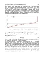
3.5 Cumulative distribution of MPY
An applicable method for comparing the extent of MPY variability among different varieties
and locations is based on their cumulative distributions, which expresses the probabilistic
climatic yield forecast (Zhukovsky et al., 1990). For the baseline climate, the late variety
‘Anti’ produced higher yields across the entire range of probabilities and the distribution of
the yield is not a symmetric one. Low yields, corresponding to extreme meteorological
conditions and forming deep deviations in time series (Fig. 5), stretch the cumulative
distribution out in the left part (Fig. 9 & 10). For the current climate, the decline in the
cumulative distribution is quite steep after the mean value of MPY. High MPY values
correspond to the years in which the different meteorological resources are well balanced
Simulated potato crop yield as an indicator of climate variability and changes in Estonia 379
Tartu 2100 A2
1
2
3
4
5

6
7
8
9
10
11
12
Year
-200
-100
0
100
200
Precipitation change,
%

Tartu 2100 B1
1
2
3
4
5
6
7
8
9
10
11
12
Year

-200
-100
0
100
200

Kuresaare 2100 A2
1
2
3
4
5
6
7
8
9
10
11
12
Year
-200
-100
0
100
200
Precipitation change,
%

Kuressaare 2100 B1
1

2
3
4
5
6
7
8
9
10
11
12
Year
-200
-100
0
100
200

Fig. 7. Changes in monthly sum of precipitation (%) predicted by 18 global climate models
for the A2 and B1 emissions scenarios for year 2100 compared to the baseline period (1961–
1990) at two Estonian sites. Lines connect the values of monthly mean change, boxes mark
mean change ± standard deviation and whiskers mark the range of all models.

3.4 MPY in the future
From now on, all changes in MPY are referred as compared to baseline period (1965-2006)
and we will discuss the yields achieved with optimal planting time. The productivity and
yield changes related to the rise of CO
2
in the atmosphere rise are not considered.
For the late variety ‘Anti’, the long-term mean MPY values, calculated by using historical

climate data of 1965-2006 with computed optimal planting time, describing the optimal
climatic resources for plant growth, are 58.9 t ha-1 in Tartu and 50.2 in Kuressaare (see Table
1). For the early variety ‘Maret’ the values are 44.0 and 39.3, respectively.
For early variety, all four considered scenarios predict losses in all given localities (Fig. 8).
Stronger scenarios cause higher losses, up to 37% in Tartu and 32% in Kuressaare by 2100.
In Kuressaare, the change in mean MPY is statistically significant for the year 2050 only by
the strongest, A2 scenario (p=0.03); for the year 2100 all scenarios predict significant loss
(p<0,001). In Tartu, for the year 2050 the change in MPY is significant by A2 (p=0.002), A1B
(p=0.01) and B2 (p=0.03) scenarios; for the year 2100, the loss in MPY is significant by all
scenarios (p<0.001).
For late variety, remote rise in yields is predicted for year 2050. Lower temperature rise
through milder scenarios is more favourable for potatoes – B1 scenario predicts 5.5% yield
rise in Tartu and 5% in Kuressaare, while for A2 scenario the rise is 2.5 and 2%. For year
2100, all scenarios predict yield losses, stronger scenarios up to 15% in Tartu, up to 19% in
Kuressaare for 2100 as compared to present climate. The changes in 'Anti' MPY are however
not statistically significant for any location, year or scenario.
Compared to yield variability in baseline climate, the predicted yield variability of 'Anti'
turned to be significantly (p<0.05) lower in Kuressaare in case of the strongest climate
change (A2 scenario for the year 2100) (standard deviation 11.6 compared to 15.8 t ha
-1
). The
'Maret' MPY variability is also lower in Kuressaare in 2100 by scenarios A1B (p<0.001), A2
(p<0.001) and B2 (p=0.02), standard deviation declining from 10.1 to 6.3, 5.7 and 7.7 t ha
-1
,
respectively. In Tartu, the change in variability was only significant (p=0.009) for A2 in 2100
(standard deviation 7.8 to 5.4 t ha
-1
).
Maret

25
30
35
40
45
50
Baseline 2050 2100
MPY t ha
-1
Anti
40
45
50
55
60
65
MPY t ha
-1
A2 Kuressaare B1 Kuressaare
A2 Tartu B1 Tartu

Fig. 8. Mean values of the meteorologically possible yield (MPY) of late potato variety ‘Anti’
and early potato variety ‘Maret’ for baseline period (1965-2006), years 2050 and 2100 by the
two scenarios predicting the strongest (A2) and weakest (B1) warming.

3.5 Cumulative distribution of MPY
An applicable method for comparing the extent of MPY variability among different varieties
and locations is based on their cumulative distributions, which expresses the probabilistic
climatic yield forecast (Zhukovsky et al., 1990). For the baseline climate, the late variety
‘Anti’ produced higher yields across the entire range of probabilities and the distribution of

the yield is not a symmetric one. Low yields, corresponding to extreme meteorological
conditions and forming deep deviations in time series (Fig. 5), stretch the cumulative
distribution out in the left part (Fig. 9 & 10). For the current climate, the decline in the
cumulative distribution is quite steep after the mean value of MPY. High MPY values
correspond to the years in which the different meteorological resources are well balanced
Climate Change and Variability380
throughout the summer period. As a rule, these are climatically similar to the climatic norms
for all the factors in Estonia. The MPY distribution for ‘Anti’ is lower in Kuressaare,
predominantly in the range of lower and central MPY values, resulting in a smoother
decline in the range of the highest yields. Even larger inequalities in mean values as well as
in their distributions appear between two locations for the early variety ‘Maret’. We can
conclude that the differences in climatic conditions during the first half of summer have a
greater effect on early varieties. The shape of the distribution curve is more symmetric for
the early variety.
Kuressaare
0,0
0,2
0,4
0,6
0,8
1,0
0 15 30 45 60 75
Meteorologically possible yield (t ha
-1
)

Mean MPY
of Anti
Tartu
0,0

0,2
0,4
0,6
0,8
1,0
0 15 30 45 60 75
Meteorologically possible yield (t ha
-1
)
Anti
Maret
Mean MPY
of Anti
Probability of MPY
Mean MPY of
Maret
Mean MPY of
Maret

Fig. 9. Cumulative distribution of the MPY for the current climate, achieved by real planting
dates.
Maret
Kuressaare
0,0
0,2
0,4
0,6
0,8
1,0
Baseline

A2 2050
B1 2050
A2 2100
B1 2100
Probability of MPY
Anti
Kuressaare
0,0
0,2
0,4
0,6
0,8
1,0
Maret
Tartu
0,0
0,2
0,4
0,6
0,8
1,0
5 15 25 35 45 55 65 75 85
Meteorologically possible yield, t ha
-1
Probability of MPY
Anti
Tartu
0,0
0,2
0,4

0,6
0,8
1,0
5 15 25 35 45 55 65 75 85
Meteorologically possible yield, t ha
-1

Fig. 10. Cumulative distribution of the MPY for baseline climate (1965-2006) and two climate
change scenarios for the target years 2050 and 2100, achieved by computed planting dates.
Cumulative distribution of the future MPY values (Fig. 10) shows greater differences
between scenarios and target years for ‘Maret’, witnessing the higher weather sensitivity of
early variety. For all cases, A2 scenario certifies definite disadvantage of strong warming
modelled for the year 2100. For ‘Anti’, the cumulative yield differences between scenarios
and target years are not very stark, enabling to conclude the advantage of longer maturing
varieties for future climate warming.

4. Conclusions and discussion
The main objective of this chapter was to show that computed yields give additional
information about climatic variability compared with the traditional use of individual
meteorological elements. Our results indicate that none of the observed separate
meteorological factors sufficiently reflects the variations in the computed MPY series. We
found significant linear correlations for only the western Estonian coastal zone, represented
by the station at Kuressaare, because of the dominant limiting factor, the water deficit
during the first half of summer in most years. Although the polynomial correlations were
higher, indicating a dual influence of the factors, there was still high variance. The
significant changes in MPY variability, as observed in Tartu in the second half of the period,
were only weakly expressed in the precipitation series and were absent from the
temperature and radiation data. Evidently, the combined effects of weather conditions on
plant production processes have a more complex character than can be measured with long-
term statistics for individual meteorological elements. Consequently, the use of MPY to

express the agrometeorological resources available for plant production in yield units
introduces additional information about the impact of climatic variability. The changes in
MPY and their statistical distribution are better indicators of the impact of climate change on
plant production than are changes in the time series of any individual meteorological
elements. This holds particularly true if simulations for species adapted to local climatic
conditions are used. If species are located at the borders of their distribution areas, some
meteorological factors will predominantly limit their growth and will describe the climatic
resources without being combined with other factors. The MPY series collected through 83-
106 years revealed no significant trends. However, significant trends do exist in terms of
shorter periods. The variability of MPY has been increasing in the island regions of Estonia
since the 1940s and in the continental areas since the 1980s.
The above-described results have been further expanded into the future and future values of
meteorologically possible potato crop yield have been generated. This allows to estimate the
influence of climate change on agrometeorological resources for potato growth in Estonia.
All of the four climate change scenarios projected the increase in annual mean temperature
for Estonia, the highest warming during the cold part of the year. Average annual
precipitation was also predicted to increase, however, changes in the annual range of
monthly precipitation vary highly between models and scenarios and are less certain than
changes in temperature. All the projected climatic tendencies have already been noted in
observations during the last century (Jaagus, 2006), indicating evident climate warming in
Estonia.
Changes in MPY were calculated using historical weather variability and projected changes
in mean monthly values. For early potato variety, all scenarios predict losses in potato
yields, while the scenarios of more notable warming cause higher losses. For late variety, a
Simulated potato crop yield as an indicator of climate variability and changes in Estonia 381
throughout the summer period. As a rule, these are climatically similar to the climatic norms
for all the factors in Estonia. The MPY distribution for ‘Anti’ is lower in Kuressaare,
predominantly in the range of lower and central MPY values, resulting in a smoother
decline in the range of the highest yields. Even larger inequalities in mean values as well as
in their distributions appear between two locations for the early variety ‘Maret’. We can

conclude that the differences in climatic conditions during the first half of summer have a
greater effect on early varieties. The shape of the distribution curve is more symmetric for
the early variety.
Kuressaare
0,0
0,2
0,4
0,6
0,8
1,0
0 15 30 45 60 75
Meteorologically possible yield (t ha
-1
)

Mean MPY
of Anti
Tartu
0,0
0,2
0,4
0,6
0,8
1,0
0 15 30 45 60 75
Meteorologically possible yield (t ha
-1
)
Anti
Maret

Mean MPY
of Anti
Probability of MPY
Mean MPY of
Maret
Mean MPY of
Maret

Fig. 9. Cumulative distribution of the MPY for the current climate, achieved by real planting
dates.
Maret
Kuressaare
0,0
0,2
0,4
0,6
0,8
1,0
Baseline
A2 2050
B1 2050
A2 2100
B1 2100
Probability of MPY
Anti
Kuressaare
0,0
0,2
0,4
0,6

0,8
1,0
Maret
Tartu
0,0
0,2
0,4
0,6
0,8
1,0
5 15 25 35 45 55 65 75 85
Meteorologically possible yield, t ha
-1
Probability of MPY
Anti
Tartu
0,0
0,2
0,4
0,6
0,8
1,0
5 15 25 35 45 55 65 75 85
Meteorologically possible yield, t ha
-1

Fig. 10. Cumulative distribution of the MPY for baseline climate (1965-2006) and two climate
change scenarios for the target years 2050 and 2100, achieved by computed planting dates.
Cumulative distribution of the future MPY values (Fig. 10) shows greater differences
between scenarios and target years for ‘Maret’, witnessing the higher weather sensitivity of

early variety. For all cases, A2 scenario certifies definite disadvantage of strong warming
modelled for the year 2100. For ‘Anti’, the cumulative yield differences between scenarios
and target years are not very stark, enabling to conclude the advantage of longer maturing
varieties for future climate warming.

4. Conclusions and discussion
The main objective of this chapter was to show that computed yields give additional
information about climatic variability compared with the traditional use of individual
meteorological elements. Our results indicate that none of the observed separate
meteorological factors sufficiently reflects the variations in the computed MPY series. We
found significant linear correlations for only the western Estonian coastal zone, represented
by the station at Kuressaare, because of the dominant limiting factor, the water deficit
during the first half of summer in most years. Although the polynomial correlations were
higher, indicating a dual influence of the factors, there was still high variance. The
significant changes in MPY variability, as observed in Tartu in the second half of the period,
were only weakly expressed in the precipitation series and were absent from the
temperature and radiation data. Evidently, the combined effects of weather conditions on
plant production processes have a more complex character than can be measured with long-
term statistics for individual meteorological elements. Consequently, the use of MPY to
express the agrometeorological resources available for plant production in yield units
introduces additional information about the impact of climatic variability. The changes in
MPY and their statistical distribution are better indicators of the impact of climate change on
plant production than are changes in the time series of any individual meteorological
elements. This holds particularly true if simulations for species adapted to local climatic
conditions are used. If species are located at the borders of their distribution areas, some
meteorological factors will predominantly limit their growth and will describe the climatic
resources without being combined with other factors. The MPY series collected through 83-
106 years revealed no significant trends. However, significant trends do exist in terms of
shorter periods. The variability of MPY has been increasing in the island regions of Estonia
since the 1940s and in the continental areas since the 1980s.

The above-described results have been further expanded into the future and future values of
meteorologically possible potato crop yield have been generated. This allows to estimate the
influence of climate change on agrometeorological resources for potato growth in Estonia.
All of the four climate change scenarios projected the increase in annual mean temperature
for Estonia, the highest warming during the cold part of the year. Average annual
precipitation was also predicted to increase, however, changes in the annual range of
monthly precipitation vary highly between models and scenarios and are less certain than
changes in temperature. All the projected climatic tendencies have already been noted in
observations during the last century (Jaagus, 2006), indicating evident climate warming in
Estonia.
Changes in MPY were calculated using historical weather variability and projected changes
in mean monthly values. For early potato variety, all scenarios predict losses in potato
yields, while the scenarios of more notable warming cause higher losses. For late variety, a
Climate Change and Variability382
slight rise in yields is predicted for 2050, which turns to loss by 2100. However, the changes
are not statistically significant for the late variety. This result is a development from
previous results with the same model (Kadaja & Tooming, 1998; Karing et al., 1999; Kadaja,
2006), which predicted yield rise with moderate scenarios for late variety and loss only
occurs with strong warming scenarios.
There have been several researches in different regions about possible climate-change-
related variation in potato growth. Peiris et al. (1996) calculated increases in tuber yield by
temperature rise for potato in Scotland due to faster crop emergence and canopy expansion
and thus a longer growth period. Wolf (1999 a, 2002) has reported small to considerable
increases in a mean tuber yield with climate change in the Northern Europe, being caused
by the higher CO
2
concentration and by the temperature rise. Wolf and van Oijen (2002)
showed yield increase for the year 2050 in all regions of the EU, mainly due to the positive
yield response to increased CO
2

. Such disagreement with our results likely derives from the
fact that in our study no effect of CO
2
rise on potato growth has been considered. There is
clear evidence since 1950s (Keeling et al., 1995) that atmospheric CO
2
is increasing, and plant
physiologists have repeatedly demonstrated that such increases likely have already caused
substantial increases in leaf photosynthesis of C
3
species (Sage, 1994). The presence of large
sinks for assimilates in tubers makes potato crop a good candidate for large growth and
yield responses to rising CO
2
; this effect tends to be smaller for late cultivars (Miglietta et al.,
2000). However, since the optimal temperature range for tuber growth (between 16 and 22
ºC) is small (Kooman, 1995), and since with climate change the prevailing temperature
during tuber growth will likely be different, the positive effect of CO
2
may be counteracted
by the effect of a concominant temperature rise. Wolf (1999a; 2002) has shown such effect for
central and southern Europe, where the negative effect of temperature rise was expected
sometimes to exceed the positive effect of CO
2
enrichment. Under hotter and wetter
scenarios for Great Britain, Wolf (1999b) demonstrated tuber yields to become lower, caused
by the temperature rise, which speeded the phenological development of the crop and
reduced the time for growth and biomass production. At the same time, under the smaller
temperature rise the yield had mainly increased at the same locations. Rosenzweig et al.
(1996) have also calculated decreases in tuber yield for most sites in the USA due to the

negative effect of temperature rise on yield that was stronger than the positive effect of CO
2

enrichment. Miglietta et al (2000) have described a model experiment for Dutch weather
conditions, where the elevated temperature reduced the positive effect of elevated CO
2
. For
predicted future temperature rise (without an increase in atmospheric CO
2
) over England
and Wales, Davies et al. (1997) calculated variable and little changes in tuber yield of potato.
Based on this knowledge and our current research result, we can thus say that the climatic
resources for potato growth are predicted to become worse under climatic change because
of increased temperature and variable rainfall; however in higher latitudes this effect may
be altered and turned positive by the change in plants photosynthetic activity and
production.
The variability of potato yields is predicted to decrease slightly due to climate change. This
is however not a plausible result, since the change in meteorological variability has not been
counted in. Further investigation need rises in this area. Also Wolf (1999a) has shown the
variability of non-irrigated tuber yield to essentially zero to moderately decrease in
Northern Europe.

Acknowledgements
Financial support from the Estonian Science Foundation grants No 6092 and 7526 is
appreciated.

5. References
Aasa, A.; Jaagus, J.; Ahas, R. & Sepp, M. (2004). The influence of atmospheric circulation on
plant phenological phases in central and eastern Europe. International Journal of
Climatology, 24 (12), 1551–1564

Adams, R.M.; Rosenzweig, C.; Peart, R.M.; Ritchie, J.T. & 6 others (1990). Global climate
change and US agriculture. Nature, 345, 219–223
Ahas, R. ; Jaagus, J. & Aasa, A. (2000). The phenological calendar of Estonia and its correlation with
mean air temperature. International Journal of Biometeorology, 44 (4), 159 – 166
Badeck, F W., Bondeau, A., Böttcher, K., Doktor, D., Lucht, W., Schaber, J. & Sitch, S. (2004).
Responses of spring phenology to climate change. New Phytologist, 162, 295–309
Barrow, E. M.; Hulme, M.; Semenov, M. A. & Brooks, R. J. (2000). Climate change scenarios.
In: Climate Change, Climatic Variability and Agriculture in Europe: an integrated
assessment, Downing, T. E.; Harrison, P. A.; Butterfield, R. E. & Londsdale, K.
G.(Eds.), 11–27, Environmental Change Institute, University of Oxford, UK
Bolin, B. (1977). Changes of Land Biota and Their Importance for the Carbon Cycle. Science,
196, 613-615
Budyko, M.I. (1971). Climate and life. Gidrometeoizdat. Leningrad. 471 pp. [in Russian, with
English abstract]
Budyko, M.I. (1974). Evolution of biosphere. Gidrometeoizdat. Leningrad. 488 pp. [in Russian,
with English abstract]
Burke, E. J.; Brown, S.J. & Christidis, N. (2006). Modeling the Recent Evolution of Global
Drought and Projections for the Twenty-First Century with the Hadley Centre
Climate Model. Journal of Hydrometeorology, 7, 1113–1125
Carter, T. R. (1996). Global climate change and agriculture in the North. Agric Food Sci
Finland, 5, 222–385
Chmielewski, F M. & Köhn, W. (2000). Impact of weather on yield and yield components of
winter rye. Agric. Forest Meteorol, 102, 253–261
Chuine, I.; Yiou, P.; Viovy, N; Seguin, B.; Daux, V. & Ladurie E.L.R. (2004). Historical
phenology: Grape ripening as a past climate indicator. Nature, 432, 289–290
Davies, A.; Jenkins, T.; Pike, A.; Shao, J.; Carson, I.; Pollock, C.J. & Parry, M.L. (1997)
Modelling the predicted geographic and economic response of UK cropping
systems to climate change scenarios: the case of potatoes. Ann Appl Biol, 130,
167–178
Donnelly, A., Jones, M.B., Sweeney, J. 2004. A review of indicators of climate change for use

in Ireland. International Journal of Biometeorology, 49, 1–12
Easterling, W.E.; McKenney, M.S.; Rosenberg, N.J. & Lemon, K.M. (1992a). Simulations of
crop response to climate change: effects with present technology and no
adjustments (the ‘dumb farmer’ scenario). Agric For Meteorol, 59, 53–73
Easterling, W.E.; Rosenberg, N.J.; Lemon, K.M. & McKenney, M.S. (1992b). Simulations of
crop responses to climate change: effects with present technology and currently
available adjustment (the ‘smart farmer’ scenario). Agric For Meteorol, 59, 75–102
Simulated potato crop yield as an indicator of climate variability and changes in Estonia 383
slight rise in yields is predicted for 2050, which turns to loss by 2100. However, the changes
are not statistically significant for the late variety. This result is a development from
previous results with the same model (Kadaja & Tooming, 1998; Karing et al., 1999; Kadaja,
2006), which predicted yield rise with moderate scenarios for late variety and loss only
occurs with strong warming scenarios.
There have been several researches in different regions about possible climate-change-
related variation in potato growth. Peiris et al. (1996) calculated increases in tuber yield by
temperature rise for potato in Scotland due to faster crop emergence and canopy expansion
and thus a longer growth period. Wolf (1999 a, 2002) has reported small to considerable
increases in a mean tuber yield with climate change in the Northern Europe, being caused
by the higher CO
2
concentration and by the temperature rise. Wolf and van Oijen (2002)
showed yield increase for the year 2050 in all regions of the EU, mainly due to the positive
yield response to increased CO
2
. Such disagreement with our results likely derives from the
fact that in our study no effect of CO
2
rise on potato growth has been considered. There is
clear evidence since 1950s (Keeling et al., 1995) that atmospheric CO
2

is increasing, and plant
physiologists have repeatedly demonstrated that such increases likely have already caused
substantial increases in leaf photosynthesis of C
3
species (Sage, 1994). The presence of large
sinks for assimilates in tubers makes potato crop a good candidate for large growth and
yield responses to rising CO
2
; this effect tends to be smaller for late cultivars (Miglietta et al.,
2000). However, since the optimal temperature range for tuber growth (between 16 and 22
ºC) is small (Kooman, 1995), and since with climate change the prevailing temperature
during tuber growth will likely be different, the positive effect of CO
2
may be counteracted
by the effect of a concominant temperature rise. Wolf (1999a; 2002) has shown such effect for
central and southern Europe, where the negative effect of temperature rise was expected
sometimes to exceed the positive effect of CO
2
enrichment. Under hotter and wetter
scenarios for Great Britain, Wolf (1999b) demonstrated tuber yields to become lower, caused
by the temperature rise, which speeded the phenological development of the crop and
reduced the time for growth and biomass production. At the same time, under the smaller
temperature rise the yield had mainly increased at the same locations. Rosenzweig et al.
(1996) have also calculated decreases in tuber yield for most sites in the USA due to the
negative effect of temperature rise on yield that was stronger than the positive effect of CO
2

enrichment. Miglietta et al (2000) have described a model experiment for Dutch weather
conditions, where the elevated temperature reduced the positive effect of elevated CO
2

. For
predicted future temperature rise (without an increase in atmospheric CO
2
) over England
and Wales, Davies et al. (1997) calculated variable and little changes in tuber yield of potato.
Based on this knowledge and our current research result, we can thus say that the climatic
resources for potato growth are predicted to become worse under climatic change because
of increased temperature and variable rainfall; however in higher latitudes this effect may
be altered and turned positive by the change in plants photosynthetic activity and
production.
The variability of potato yields is predicted to decrease slightly due to climate change. This
is however not a plausible result, since the change in meteorological variability has not been
counted in. Further investigation need rises in this area. Also Wolf (1999a) has shown the
variability of non-irrigated tuber yield to essentially zero to moderately decrease in
Northern Europe.

Acknowledgements
Financial support from the Estonian Science Foundation grants No 6092 and 7526 is
appreciated.

5. References
Aasa, A.; Jaagus, J.; Ahas, R. & Sepp, M. (2004). The influence of atmospheric circulation on
plant phenological phases in central and eastern Europe. International Journal of
Climatology, 24 (12), 1551–1564
Adams, R.M.; Rosenzweig, C.; Peart, R.M.; Ritchie, J.T. & 6 others (1990). Global climate
change and US agriculture. Nature, 345, 219–223
Ahas, R. ; Jaagus, J. & Aasa, A. (2000). The phenological calendar of Estonia and its correlation with
mean air temperature. International Journal of Biometeorology, 44 (4), 159 – 166
Badeck, F W., Bondeau, A., Böttcher, K., Doktor, D., Lucht, W., Schaber, J. & Sitch, S. (2004).
Responses of spring phenology to climate change. New Phytologist, 162, 295–309

Barrow, E. M.; Hulme, M.; Semenov, M. A. & Brooks, R. J. (2000). Climate change scenarios.
In: Climate Change, Climatic Variability and Agriculture in Europe: an integrated
assessment, Downing, T. E.; Harrison, P. A.; Butterfield, R. E. & Londsdale, K.
G.(Eds.), 11–27, Environmental Change Institute, University of Oxford, UK
Bolin, B. (1977). Changes of Land Biota and Their Importance for the Carbon Cycle. Science,
196, 613-615
Budyko, M.I. (1971). Climate and life. Gidrometeoizdat. Leningrad. 471 pp. [in Russian, with
English abstract]
Budyko, M.I. (1974). Evolution of biosphere. Gidrometeoizdat. Leningrad. 488 pp. [in Russian,
with English abstract]
Burke, E. J.; Brown, S.J. & Christidis, N. (2006). Modeling the Recent Evolution of Global
Drought and Projections for the Twenty-First Century with the Hadley Centre
Climate Model. Journal of Hydrometeorology, 7, 1113–1125
Carter, T. R. (1996). Global climate change and agriculture in the North. Agric Food Sci
Finland, 5, 222–385
Chmielewski, F M. & Köhn, W. (2000). Impact of weather on yield and yield components of
winter rye. Agric. Forest Meteorol, 102, 253–261
Chuine, I.; Yiou, P.; Viovy, N; Seguin, B.; Daux, V. & Ladurie E.L.R. (2004). Historical
phenology: Grape ripening as a past climate indicator. Nature, 432, 289–290
Davies, A.; Jenkins, T.; Pike, A.; Shao, J.; Carson, I.; Pollock, C.J. & Parry, M.L. (1997)
Modelling the predicted geographic and economic response of UK cropping
systems to climate change scenarios: the case of potatoes. Ann Appl Biol, 130,
167–178
Donnelly, A., Jones, M.B., Sweeney, J. 2004. A review of indicators of climate change for use
in Ireland. International Journal of Biometeorology, 49, 1–12
Easterling, W.E.; McKenney, M.S.; Rosenberg, N.J. & Lemon, K.M. (1992a). Simulations of
crop response to climate change: effects with present technology and no
adjustments (the ‘dumb farmer’ scenario). Agric For Meteorol, 59, 53–73
Easterling, W.E.; Rosenberg, N.J.; Lemon, K.M. & McKenney, M.S. (1992b). Simulations of
crop responses to climate change: effects with present technology and currently

available adjustment (the ‘smart farmer’ scenario). Agric For Meteorol, 59, 75–102
Climate Change and Variability384
Fritts, H.C. (1976). Tree Rings and Climate. Academic Press, London
Hafner, S. (2003). Trends in maize, rice, and wheat yields for 188 nations over the past 40
years: a prevalence of linear growth, Agriculture, Ecosystems & Environment, 97,
275 – 283
Hay, R.K.M. & Porter J.R. (2006). The physiology of crop yield. 2nd ed., Blackwell Publishing,
UK
Hulme, M.; Wigley, T.M.L.; Barrow, E.M.; Raper, S.C.B.; Centella, A.; Smith, S.J. &
Chipanshi, A.C. (2000). Using a Climate Scenario Generator for Vulnerability and
Adaptation Assessments: MAGICC and SCENGEN Version 2.4 Workbook. Climatic
Research Unit, Norwich UK
Hurrell, J.W. & van Loon H. (1997). Decadal variations in climate associated with the North
Atlantic Oscillation. Clim Change, 36, 301–326
IPCC (2007). Climate Change 2007: The Physical Science Basis. In: Contribution of Working
Group I to the Fourth Assessment Report of the Intergovernmental Panel on Climate
Change. Solomon, S., D. Qin, M. Manning, Z. Chen, M. Marquis, K.B. Averyt, M.
Tignor & H.L. Miller (Eds.). Cambridge University Press, Cambridge, UK and New
York
Jaagus, J. (2006). Climatic changes in Estonia during the second half of the 20th century in
relationship with changes in large-scale atmospheric circulation. Theor. Appl.
Climatol, 83, 77–88
Jaagus, J. & Truu J. (2004). Climatic regionalisation of Estonia based on multivariate
exploratory techniques. Estonia. Geographical studies, 9, 41–55
Kadaja, J. (1994). Agrometeorological resources for a concrete agricultural crop expressed in
the yield units and their territorial distribution for potato. In: Proceedings of the GIS
— Baltic Sea States 93, Vilu H., Vilu R. (Eds.), 139–149, Tallinn Technical University,
Tallinn
Kadaja, J. (2004). Influence of fertilisation on potato growth functions. Agronomy Research,
2(1), 49-55

Kadaja, J. (2006). Reaction of potato yield to possible climate change in Estonia. Book of
proceedings. IX ESA Congress. Part I. Bibliotheca Fragmenta Agronomica 11, Fotyma, M.
& Kaminska B. (eds.), 297–298, Pulawy–Warszawa
Kadaja, J. & Tooming, H. (1998). Climate change scenarios and agricultural crop yields. In:
Country case study on climate change impacts and adaptation assessments in the Republic
of Estonia, Tarand, A. & Kallaste, T. (Eds.), 39–41, Ministry of the Environment
Republic of Estonia, SEI, CEF, UNEP, Tallinn
Kadaja, J. & Tooming, H. (2004) Potato production model based on principle of maximum
plant productivity, Agric. For. Meteorology, 127 (1–2), 17–33
Karing, P.; Kallis, A & Tooming, H. (1999). Adaptation principles of agriculture to climate
change. Clim Res, 12, 175–183
Keeling, C.D.; Whorf, T.P.; Whalen, M. & van der Plicht, J. (1995). Interannual extremes in
the rate of rise of atmospheric carbon dioxide since 1980. Nature, 375, 666–670
Keevallik, S. (1998). Climate change scenarios for Estonia. In: Country case study on climate
change impacts and adaptation assessments in the Republic of Estonia, Tarand, A. &
Kallaste, T. (Eds.), 1–6, Ministry of the Environment Republic of Estonia, SEI, CEF,
UNEP, Tallinn
Kitse, E. (1978). Mullavesi [Soil water]. Tallinn, Valgus [in Estonian]
Kont, A.; Jaagus, J. & Aunap, R. (2003). Climate change scenarios and the effect of sea-level
rise for Estonia. Global and Planetary Change, 36, 1 –15
Kooman, P.L. (1995).Yielding ability of potato crops as influenced by temperature and daylength.
PhD thesis, Wageningen Agricultural University, Wageningen, The Netherlands
Makra, L.; Horváth, S.; Pongrácz R.& Mika, J. (2002). Long term climate deviations: an
alternative approach and application on the Palmer drought severity index in
Hungary, Physics and Chemistry of the Earth, 27, 1063–1071
McPherson, R. (2007). A review of vegetation—atmosphere interactions and their influences
on mesoscale phenomena. Progress in Physical Geography, 31, 261-285
Mearns, L.O. ( 2000). Climate change and variability. In: Climate Change and Global Crop
Productivity. Reddy, K.R. & Hodges, H.F. (Eds.), 7–35, CAB International Publishing
Mela, T. (1996). Northern agriculture: constraints and responses to global climate change.

Agricultural and Food Science in Finland, 5 (3), 229–234
Menzel, A. (2003). Plant Phenological Anomalies in Germany and their Relation to Air Temperature
and NAO. Climatic Change, 57 (3), 243–263
Menzel, A. & Fabian, P. (1999). Growing season extended in Europe. Nature, 397, 659
Miglietta, F.; Bindi, M.; Vaccari, F.P.; Schapendonk, A.H.C.M.; Wolf, J.; Butterfield, R.E.
(2000). Crop Ecosystem Responses to Climatic Change: Root and Tuberous Crops.
In: Climate Change and Global Crop productivity. Reddy, K.R; Hodges, H.F (Eds.).
CAB International Publishing
Mpelasoka, F.; Hennessy. K., Jones R. & Bates B. (2007). Comparison of suitable drought
indices for climate change impacts assessment over Australia towards resource
management. International Journal of Climatology, 28, 1283–1292
Nakićenović, N. & Swart, R. (Eds.). (2000). Special Report on Emissions Scenarios. Cambridge
University Press, Cambridge, UK, 570 pp.
Peiris, D.R.; Crawford, J.W.; Grashoff, C.; Jefferies, R.A.; Porter, J.R. & Marshall, B. (1996). A
simulation study of crop growth and development under climate change. Agric For
Meteorol, 79, 271–287
Pensa, M.; Sepp, M. & Jalkanen, R. (2006). Connections between climatic variables and the
growth and needle dynamics of Scots pine (Pinus sylvestris L.) in Estonia and
Lapland. International Journal of Biometeorology, 50 (4), 205–214
Rind, D.; Goldberg, R. & Ruedy, R. (1989). Change in climate variability in the 21st century.
Clim Change, 14, 5–37
Rosenzweig, C.; Phillips, J.; Goldberg, R.; Carroll, J. & Hodges, T. (1996). Potential impacts of
climate change on citrus and potato production in the US. Agric Syst, 52, 455–479
Ross J. (1966). About the mathematical description of plant growth. DAN SSSR 171 (2b),
481–483 [In Russian]
Sage, R.F. (1994). Acclimation of photosynthesis to increasing atmospheric CO
2
. The gas
exchange perspective. Photosynthesis Research, 39, 351–368
Santer, B.D.; Wigley, T.M.L.; Schlesinger, M.E. & Mitchell, J.F.B. (1990). Developing Climate

Scenarios from Equilibrium GCM Results. Max-Planck-Institut für Meteorologie
Report No. 47, Hamburg, Germany
Saue, T. (2006). Site-specific information and determination of parameters for a plant production
process model. Masters thesis. Eurouniversity, Tallinn.
Saue, T.; Kadaja, J. (2009). Simulated crop yield - an indicator of climate variability. Boreal
Environment Research, 14(1), 132–142.
Simulated potato crop yield as an indicator of climate variability and changes in Estonia 385
Fritts, H.C. (1976). Tree Rings and Climate. Academic Press, London
Hafner, S. (2003). Trends in maize, rice, and wheat yields for 188 nations over the past 40
years: a prevalence of linear growth, Agriculture, Ecosystems & Environment, 97,
275 – 283
Hay, R.K.M. & Porter J.R. (2006). The physiology of crop yield. 2nd ed., Blackwell Publishing,
UK
Hulme, M.; Wigley, T.M.L.; Barrow, E.M.; Raper, S.C.B.; Centella, A.; Smith, S.J. &
Chipanshi, A.C. (2000). Using a Climate Scenario Generator for Vulnerability and
Adaptation Assessments: MAGICC and SCENGEN Version 2.4 Workbook. Climatic
Research Unit, Norwich UK
Hurrell, J.W. & van Loon H. (1997). Decadal variations in climate associated with the North
Atlantic Oscillation. Clim Change, 36, 301–326
IPCC (2007). Climate Change 2007: The Physical Science Basis. In: Contribution of Working
Group I to the Fourth Assessment Report of the Intergovernmental Panel on Climate
Change. Solomon, S., D. Qin, M. Manning, Z. Chen, M. Marquis, K.B. Averyt, M.
Tignor & H.L. Miller (Eds.). Cambridge University Press, Cambridge, UK and New
York
Jaagus, J. (2006). Climatic changes in Estonia during the second half of the 20th century in
relationship with changes in large-scale atmospheric circulation. Theor. Appl.
Climatol, 83, 77–88
Jaagus, J. & Truu J. (2004). Climatic regionalisation of Estonia based on multivariate
exploratory techniques. Estonia. Geographical studies, 9, 41–55
Kadaja, J. (1994). Agrometeorological resources for a concrete agricultural crop expressed in

the yield units and their territorial distribution for potato. In: Proceedings of the GIS
— Baltic Sea States 93, Vilu H., Vilu R. (Eds.), 139–149, Tallinn Technical University,
Tallinn
Kadaja, J. (2004). Influence of fertilisation on potato growth functions. Agronomy Research,
2(1), 49-55
Kadaja, J. (2006). Reaction of potato yield to possible climate change in Estonia. Book of
proceedings. IX ESA Congress. Part I. Bibliotheca Fragmenta Agronomica 11, Fotyma, M.
& Kaminska B. (eds.), 297–298, Pulawy–Warszawa
Kadaja, J. & Tooming, H. (1998). Climate change scenarios and agricultural crop yields. In:
Country case study on climate change impacts and adaptation assessments in the Republic
of Estonia, Tarand, A. & Kallaste, T. (Eds.), 39–41, Ministry of the Environment
Republic of Estonia, SEI, CEF, UNEP, Tallinn
Kadaja, J. & Tooming, H. (2004) Potato production model based on principle of maximum
plant productivity, Agric. For. Meteorology, 127 (1–2), 17–33
Karing, P.; Kallis, A & Tooming, H. (1999). Adaptation principles of agriculture to climate
change. Clim Res, 12, 175–183
Keeling, C.D.; Whorf, T.P.; Whalen, M. & van der Plicht, J. (1995). Interannual extremes in
the rate of rise of atmospheric carbon dioxide since 1980. Nature, 375, 666–670
Keevallik, S. (1998). Climate change scenarios for Estonia. In: Country case study on climate
change impacts and adaptation assessments in the Republic of Estonia, Tarand, A. &
Kallaste, T. (Eds.), 1–6, Ministry of the Environment Republic of Estonia, SEI, CEF,
UNEP, Tallinn
Kitse, E. (1978). Mullavesi [Soil water]. Tallinn, Valgus [in Estonian]
Kont, A.; Jaagus, J. & Aunap, R. (2003). Climate change scenarios and the effect of sea-level
rise for Estonia. Global and Planetary Change, 36, 1 –15
Kooman, P.L. (1995).Yielding ability of potato crops as influenced by temperature and daylength.
PhD thesis, Wageningen Agricultural University, Wageningen, The Netherlands
Makra, L.; Horváth, S.; Pongrácz R.& Mika, J. (2002). Long term climate deviations: an
alternative approach and application on the Palmer drought severity index in
Hungary, Physics and Chemistry of the Earth, 27, 1063–1071

McPherson, R. (2007). A review of vegetation—atmosphere interactions and their influences
on mesoscale phenomena. Progress in Physical Geography, 31, 261-285
Mearns, L.O. ( 2000). Climate change and variability. In: Climate Change and Global Crop
Productivity. Reddy, K.R. & Hodges, H.F. (Eds.), 7–35, CAB International Publishing
Mela, T. (1996). Northern agriculture: constraints and responses to global climate change.
Agricultural and Food Science in Finland, 5 (3), 229–234
Menzel, A. (2003). Plant Phenological Anomalies in Germany and their Relation to Air Temperature
and NAO. Climatic Change, 57 (3), 243–263
Menzel, A. & Fabian, P. (1999). Growing season extended in Europe. Nature, 397, 659
Miglietta, F.; Bindi, M.; Vaccari, F.P.; Schapendonk, A.H.C.M.; Wolf, J.; Butterfield, R.E.
(2000). Crop Ecosystem Responses to Climatic Change: Root and Tuberous Crops.
In: Climate Change and Global Crop productivity. Reddy, K.R; Hodges, H.F (Eds.).
CAB International Publishing
Mpelasoka, F.; Hennessy. K., Jones R. & Bates B. (2007). Comparison of suitable drought
indices for climate change impacts assessment over Australia towards resource
management. International Journal of Climatology, 28, 1283–1292
Nakićenović, N. & Swart, R. (Eds.). (2000). Special Report on Emissions Scenarios. Cambridge
University Press, Cambridge, UK, 570 pp.
Peiris, D.R.; Crawford, J.W.; Grashoff, C.; Jefferies, R.A.; Porter, J.R. & Marshall, B. (1996). A
simulation study of crop growth and development under climate change. Agric For
Meteorol, 79, 271–287
Pensa, M.; Sepp, M. & Jalkanen, R. (2006). Connections between climatic variables and the
growth and needle dynamics of Scots pine (Pinus sylvestris L.) in Estonia and
Lapland. International Journal of Biometeorology, 50 (4), 205–214
Rind, D.; Goldberg, R. & Ruedy, R. (1989). Change in climate variability in the 21st century.
Clim Change, 14, 5–37
Rosenzweig, C.; Phillips, J.; Goldberg, R.; Carroll, J. & Hodges, T. (1996). Potential impacts of
climate change on citrus and potato production in the US. Agric Syst, 52, 455–479
Ross J. (1966). About the mathematical description of plant growth. DAN SSSR 171 (2b),
481–483 [In Russian]

Sage, R.F. (1994). Acclimation of photosynthesis to increasing atmospheric CO
2
. The gas
exchange perspective. Photosynthesis Research, 39, 351–368
Santer, B.D.; Wigley, T.M.L.; Schlesinger, M.E. & Mitchell, J.F.B. (1990). Developing Climate
Scenarios from Equilibrium GCM Results. Max-Planck-Institut für Meteorologie
Report No. 47, Hamburg, Germany
Saue, T. (2006). Site-specific information and determination of parameters for a plant production
process model. Masters thesis. Eurouniversity, Tallinn.
Saue, T.; Kadaja, J. (2009). Simulated crop yield - an indicator of climate variability. Boreal
Environment Research, 14(1), 132–142.
Climate Change and Variability386
Saue, T.; Viil, P.; Kadaja, J. (2010). Do different tillage and fertilization methods influence
weather risk on potato yield? Agronomy Research, xx–xx [in press]
Scheifinger, H.; Menzel, A.; Koch, E.; Peter, C.; Ahas, R. (2002). Atmospheric mechanisms
governing the spatial and temporal variability of phenological phases in central
Europe. International Journal of Climatology, 22, 1739–1755
Schwarz, M.D.; Reiter, B.E. (2000). Changes in North American spring. Int. J. Biometeorol, 20,
929–932
Semenov, M.A.; Porter, J.R. ( 1995). Climatic variability and the modelling of crop yields.
Journal of Agricultural and Forest Meteorology, 73, 265–283
Semenov, M.A.; Wolf, J.; Evans, L.G.; Eckersten, H.; Iglesias, A. (1996). Comparison of wheat
simulation models under climate change. II. Application of climate change
scenarios. Climate Research, 7, 271–281
Sepp J.; Tooming, H. & Shvetsova, V.M. (1989). Comparative assessment of potato
productivity in the Komi A.S.S.R. and in Baltic republics by the method of dynamic
modeling. Fiziologija Rastenii (Plant Physiology) 36 (1), 68–75 [In Russian with
English summary]
Sepp J. & Tooming, H. (1991). Productivity resources of potato, Gidrometeoizdat, Leningrad [in
Russian with English abstract]

Sparks, T. & Tryjanowski, P. (2007). Patterns of spring arrival dates differ in two hirundines.
Climate Research, 35, 159–164
Sparks, T.H., Jeffree, E.P. & Jeffree, C.E., (2000). An examination of the relationship between
owering times and temperature at the national scale using long-term phonological
records from the UK. Int. J. Biometeorol. 44, 82–87
Szep I.J.; Mika J.; Dunkel Z. (2005). Palmer drought severity index as soil moisture indicator:
Physical interpretation, statistical behaviour and relation to global climate. Physics
and Chemistry of the Earth, 30 (1-3 SPEC. ISS.), 231–243
Tooming, H. (1967). Mathematical model of plant photosynthesis considering adaptation.
Photosynthetica, 1 (3 - 4), 233–240
Tooming, H. (1970). Mathematical description of net photosynthesis and adaptation
processes in the photosynthetic apparatus of plant communities. In: Prediction and
Measurement of Photosynthetic Productivity. Setlik I. (Ed.), 103–114, Pudoc,
Wageningen
Tooming, H. (1977). Solar radiation and yield formation. Gidrometeoizdat, Leningrad [In
Russian with English abstract]
Tooming, H. (1984). Ecological principles of maximum crop productivity. Gidrometeoizdat,
Leningrad [in Russian with English summary].
Tooming, H. (1988). Principle of maximum plant productivity. In: Lectures in Theoretical
Biology. Kull K., Tiivel T. (Eds.),. 129–138, Valgus, Tallinn
Tooming, H. (1993). Evaluation of agrometeorological resources based on the potential
productivity of crops. Journ. Agric. Met. (Jap.) 48 (5), 501–507
Tooming, H. (1998). Climate change and estimation of ecologically founded yields. In:
Climate change studies in Estonia, Kallaste, T., Kuldna, P. (Eds). 141–152, Stockholm
Environment Institute Tallinn Centre – Ministry of environment, Republic of
Estonia, Tallinn
Tooming, H. & Kadaja, J. (1999). Climate changes indicated by trends in snow cover
duration and surface albedo in Estonia. Meteorol Zeitschrift, 8, 16–21
Tooming, H. & Kadaja, J. (2006). Relationships of snow cover in Estonian climate – relations
from winter to spring. In: Handbook of Estonian snow cover. Tooming, H. & Kadaja, J.

(Compilers), Kallis A. (Ed.),. 112–133. Estonian Meteorological and Hydrological
Institute – Estonian Research Institute of Agriculture, Tallinn – Saku
Wolf, J. (1999a). Modelling climate change impacts at the site scale on potato. In: Climate
Change, Climate variability and Agriculture in Europe: an integrated assessment. Report
No. 21. Downing, T.E.; Harrison, P.A.; Butterfield, R.E.; Lonsdale, K.G. (Eds.). 135–
154, Environmental Change Unit, University of Oxford, Oxford, UK
Wolf, J. (1999b). Modelling climate change impacts on potato in central England. In: Climate
Change, Climate variability and Agriculture in Europe: an integrated assessment. Report
No. 21. Downing, T.E.; Harrison, P.A.; Butterfield, R.E.; Lonsdale, K.G. (Eds.), 239–
261, Environmental Change Unit, University of Oxford, Oxford, UK
Wolf J. (2002) Comparison of two potato simulation models under climate change. II.
Application of climate change scenarios. Clim Res, 21, 187–198
Wolf, J. & van Oijen, M. (2002). Modelling the dependence of European potato yields on
changes in climate and CO
2.
Agricultural and Forest Meteorology, 112 (3-4), 217-231
Woodward, F.I. (1988). Temperature and the distribution of plant species and vegetation. In:
Plants and Temperature, Long S.P and Woodward F.I. (Eds), 59 –75, Society of
Experimental Biology by The Company of Biologists Limited, Cambridge
Zhukovsky, E.E., Sepp J. & Tooming, H. (1989). On the possibility of the yield calculation
forecasting calculation. Vestn. S H. Nauki (Messenger of agricultural sciences) (5), 68-
79 [In Russian with English abstract]
Zhukovsky, E.E., Sepp J. & Tooming, H. (1990). Probabilistic forecasts of possible yield.
Meteorologija i Gidrologiya (Meteorology and Hydrology) (1), 95-102 [In Russian with
English abstract].
Simulated potato crop yield as an indicator of climate variability and changes in Estonia 387
Saue, T.; Viil, P.; Kadaja, J. (2010). Do different tillage and fertilization methods influence
weather risk on potato yield? Agronomy Research, xx–xx [in press]
Scheifinger, H.; Menzel, A.; Koch, E.; Peter, C.; Ahas, R. (2002). Atmospheric mechanisms
governing the spatial and temporal variability of phenological phases in central

Europe. International Journal of Climatology, 22, 1739–1755
Schwarz, M.D.; Reiter, B.E. (2000). Changes in North American spring. Int. J. Biometeorol, 20,
929–932
Semenov, M.A.; Porter, J.R. ( 1995). Climatic variability and the modelling of crop yields.
Journal of Agricultural and Forest Meteorology, 73, 265–283
Semenov, M.A.; Wolf, J.; Evans, L.G.; Eckersten, H.; Iglesias, A. (1996). Comparison of wheat
simulation models under climate change. II. Application of climate change
scenarios. Climate Research, 7, 271–281
Sepp J.; Tooming, H. & Shvetsova, V.M. (1989). Comparative assessment of potato
productivity in the Komi A.S.S.R. and in Baltic republics by the method of dynamic
modeling. Fiziologija Rastenii (Plant Physiology) 36 (1), 68–75 [In Russian with
English summary]
Sepp J. & Tooming, H. (1991). Productivity resources of potato, Gidrometeoizdat, Leningrad [in
Russian with English abstract]
Sparks, T. & Tryjanowski, P. (2007). Patterns of spring arrival dates differ in two hirundines.
Climate Research, 35, 159–164
Sparks, T.H., Jeffree, E.P. & Jeffree, C.E., (2000). An examination of the relationship between
owering times and temperature at the national scale using long-term phonological
records from the UK. Int. J. Biometeorol. 44, 82–87
Szep I.J.; Mika J.; Dunkel Z. (2005). Palmer drought severity index as soil moisture indicator:
Physical interpretation, statistical behaviour and relation to global climate. Physics
and Chemistry of the Earth, 30 (1-3 SPEC. ISS.), 231–243
Tooming, H. (1967). Mathematical model of plant photosynthesis considering adaptation.
Photosynthetica, 1 (3 - 4), 233–240
Tooming, H. (1970). Mathematical description of net photosynthesis and adaptation
processes in the photosynthetic apparatus of plant communities. In: Prediction and
Measurement of Photosynthetic Productivity. Setlik I. (Ed.), 103–114, Pudoc,
Wageningen
Tooming, H. (1977). Solar radiation and yield formation. Gidrometeoizdat, Leningrad [In
Russian with English abstract]

Tooming, H. (1984). Ecological principles of maximum crop productivity. Gidrometeoizdat,
Leningrad [in Russian with English summary].
Tooming, H. (1988). Principle of maximum plant productivity. In: Lectures in Theoretical
Biology. Kull K., Tiivel T. (Eds.),. 129–138, Valgus, Tallinn
Tooming, H. (1993). Evaluation of agrometeorological resources based on the potential
productivity of crops. Journ. Agric. Met. (Jap.) 48 (5), 501–507
Tooming, H. (1998). Climate change and estimation of ecologically founded yields. In:
Climate change studies in Estonia, Kallaste, T., Kuldna, P. (Eds). 141–152, Stockholm
Environment Institute Tallinn Centre – Ministry of environment, Republic of
Estonia, Tallinn
Tooming, H. & Kadaja, J. (1999). Climate changes indicated by trends in snow cover
duration and surface albedo in Estonia. Meteorol Zeitschrift, 8, 16–21
Tooming, H. & Kadaja, J. (2006). Relationships of snow cover in Estonian climate – relations
from winter to spring. In: Handbook of Estonian snow cover. Tooming, H. & Kadaja, J.
(Compilers), Kallis A. (Ed.),. 112–133. Estonian Meteorological and Hydrological
Institute – Estonian Research Institute of Agriculture, Tallinn – Saku
Wolf, J. (1999a). Modelling climate change impacts at the site scale on potato. In: Climate
Change, Climate variability and Agriculture in Europe: an integrated assessment. Report
No. 21. Downing, T.E.; Harrison, P.A.; Butterfield, R.E.; Lonsdale, K.G. (Eds.). 135–
154, Environmental Change Unit, University of Oxford, Oxford, UK
Wolf, J. (1999b). Modelling climate change impacts on potato in central England. In: Climate
Change, Climate variability and Agriculture in Europe: an integrated assessment. Report
No. 21. Downing, T.E.; Harrison, P.A.; Butterfield, R.E.; Lonsdale, K.G. (Eds.), 239–
261, Environmental Change Unit, University of Oxford, Oxford, UK
Wolf J. (2002) Comparison of two potato simulation models under climate change. II.
Application of climate change scenarios. Clim Res, 21, 187–198
Wolf, J. & van Oijen, M. (2002). Modelling the dependence of European potato yields on
changes in climate and CO
2.
Agricultural and Forest Meteorology, 112 (3-4), 217-231

Woodward, F.I. (1988). Temperature and the distribution of plant species and vegetation. In:
Plants and Temperature, Long S.P and Woodward F.I. (Eds), 59 –75, Society of
Experimental Biology by The Company of Biologists Limited, Cambridge
Zhukovsky, E.E., Sepp J. & Tooming, H. (1989). On the possibility of the yield calculation
forecasting calculation. Vestn. S H. Nauki (Messenger of agricultural sciences) (5), 68-
79 [In Russian with English abstract]
Zhukovsky, E.E., Sepp J. & Tooming, H. (1990). Probabilistic forecasts of possible yield.
Meteorologija i Gidrologiya (Meteorology and Hydrology) (1), 95-102 [In Russian with
English abstract].
Climate Change and Variability388
Determining the relationship between climate
variations and wine quality: the WEBSOM approach 389
Determining the relationship between climate variations and wine quality:
the WEBSOM approach
Subana Shanmuganathan and Philip Sallis
x

Determining the relationship between
climate variations and wine quality:
the WEBSOM approach

Subana Shanmuganathan and Philip Sallis
Auckland University of Technology
New Zealand

1. Introduction
Climate change has the potential to impact on all forms of agriculture and vegetation and the
impact is predicted to be inconsistent across the globe. Thus the polarising debates on climate
change, the phenomenon that has become to be famously known as ‘global warming’ or ‘global
climate change’, has increased scientific and commercial interest immensely in this topic and

predictions relating to it. The potential influence of climate variation on viticulture and enology is
considered to be dramatic because grapevine varieties are among the most sensitive cultivated
crops that thrive only under niche climate and environmental conditions. Historical viticulture
records evidence the fact that the winemaker ability to produce premium quality wine is highly
influenced by the environment and climate apart from the grapevine variety itself as described
by a famous Mediterranean concept “Terrior x cultiva”. Major variations in climate can even force
shifts in whole wine regions. Minor or seasonal variations generally result in differences in
quality among vintages. The historical data on the factors relating to climate and wine quality is
proving invaluable in comparing contemporary data with the past and it is essential for any
forecasting or prediction over time (Hansen, et al., 2001: Jones, 2005).
Literature reviewed for this research reveals that in the past viticulturists and winemakers
introduced and developed subtle changes to cultivation practices and winemaking processes to
turn the annual (or vintage-to-vintage) climate change effects, favourable for winemaking. This
has been occurring over centuries to turn climate variation effects to grapevine growing
advantage in an endeavour to produce finer wine labels. On the other hand, major shifts in
cultivation methods in whole wine-producing regions have occurred in the past and it appears
that all these happened in order to produce grapes with a higher percentage of sugar but without
comprising the other aroma and colour pro-protein compounds in the berry ripening process.
These characteristics of wine quality are considered to be the principal factors relating to climate
for viticulture regions throughout the world. Irrigation, frost, wind and solar influences are also
major factors in grape production and therefore, primary determinants of wine quality (Jones,
2005).
In view of the above facts, approaches based on modern knowledge discovery methods are now
being increasingly investigated to improving our understanding on climate and environmental
influences on wine quality. Sections 2 and 3 illustrate on some of the literature and our related
20
Climate Change and Variability390

research in modelling wine quality using sensory data in both text and numeric formats. Section
3 details on the other novel methods being experimented at the Geoinformatics Research Centre

(GRC), Auckland University of Technology (AUT) in New Zealand, to modelling the blended
quantitative and qualitative grapevine phenology data that determines the sugar and protein
components in grapes and its influence on the final wine product. Initial results of this research
are outlined in this section. Consequently, the WEBSOM approach to mining unstructured data
in other major problem domains is outlined. Section 4 illustrates the WEBSOM approach being
investigated in the Centre to analysing sommelier comments in free text format with sample data
set, extracted from a web magazine (Wine enthusiast, 2009), with an ultimate aim of modelling
the climate change effects on grapevine phenology and wine quality. The final section proposes
future research to model the effects of climate change in greater detail with larger data sets from
more grape growing regions within New Zealand and Chile to study the climate change effects
on the world’s major wine regions in the southern hemisphere. From this analysis we expect to
be able to predict the wine quality, style and appellations suitable for future climate change,
short-/long-term, with data from climate models already developed.

2. The effects of climate change
Climate change is predicted to bring about significant modifications to all forms of
agriculture and vegetation on earth at varying degrees (Atkins, et al., 2006). Its potential
impact on Viticulture, the world’s old and most expensive cultivated crop and enology based
on the science that underpins it, is considered by many observers to be dramatic (Jones, et al.,
2005). The recent model predictions relating to future climate change suggest that the effects
to be inconsistent across the globe (severe in the northern hemisphere and mild in the
southern) and also, to have a variable effect on different grapevine varieties. Grapevine
phonology, such as crop budburst, floraison, veraison, and harvest, greatly depends on local
weather conditions in different regions, and this is a major factor in determining wine
vintage quality. For example, even over a single degree centigrade change in temperature is
predicted to make the production of the world’s famous Mediterranean wine appellations
impossible. Grape varieties thrive under significantly narrow or niche climate and
environmental conditions, and historical evidence as well suggests that the production of
premium quality wine labels as highly prone to any change in current climate, annual as
well as long term. Research findings with Australian grapevines and wines (Web, 2006)

suggest that a change of grapevine varieties could be a way to overcome the effects of future
climate change in that country’s major wine regions. This would of course, be an extremely
expensive exercise (Gutierrez, 2005), which is why objective scientific analysis for scenario
building and prediction is of great significance at the moment.
The research discussed in this paper relates to the overarching research project, Eno-
Humanas (www.geo-informatics.org) that is aimed at building models based on correlations
between dependent and independent sets of diffident combinatorial data collected on the
environment, climate and atmosphere, soil, terrain, moisture and plant responses in
association with sensory perception data relating to flavour, odour and fruit robustness
(Sallis, et al., 2008 : Shanmuganathan, et al., 2008). Hence, the title Eno-Humanas, is about the
combination of precise ecological data and the less precise qualitative opinion data that
comes from wine consumers. This paper relates to the imprecise data analysis aspect in that
it analyses the descriptions of wine quality coming from experts; Master Wine Sommeliers.

3. Modelling grape wine using text based comments
This section of the chapter outlines some major methodologies from the literature on this
topic and then discusses GRC research in wine quality and sensory data analysis. Finally,
the WEBSOM approach and its applications are discussed.

3.1 Wine sensory analysis
The wine quality literature relating to sensory and chemical data analysis can be broadly
categorised into the following:
1) Wine characterisation and discrimination using chemical and sensory properties:
Most of the papers reviewed fall into this category. Wine of all main appellations, for
example, champagne, chardonnay, and pinot noir, have been analysed with chemical
sensory analyses, in search of better ways to identify the differences between the
wines for use in classifying sub-appellations within the main ones. For example, in
(Parr, et al., 2007) a distinctive New Zealand wine style Marlborough Sauvignon
Blanc was classified by sensory characterisation and chemical analysis for selected
aroma compounds for that wine type. In (Kontkanen, 2005) the differences that

might be supportive for designating three sub-appellations of red Niagara Peninsula
Bordeaux style were investigated using chemical and sensory analysis on forty-one
commercially available wines. Similarly, (Vannier, et al., 1999) and (Gawel, 2001)
looked at strategies a) to control champagne wine quality based on sensory and b)
red table wine quality characterised by pleasing and complex mouth-feel sensations
respectively.
2) Professional versus novice taster abilities. There are many studies in this area cited in
the literature and another project within Eno-Humanas is considering this from an
audio-mining perspective to elicit the degree of emphasis (passion) expressed about
wine quality in recording of wine tasting by both professionals and novices.
3) Wine ratings, favourable climatic conditions and price fluctuations. Research on this
subject described by Jones, et al., (2005) looked at climate and global wine quality
factors and discussed a year-to-year comparison over a ten year period. It includes a
description of wine quality factors in juxtaposition with prices and vintage ratings.
Citing many earlier studies the authors of this work pointed out that the analysis of
the relationships between climate variables and wine prices to be based on an
underlying hypothesis that beneficial climate conditions would improve the wine
quality and that in the past, these had in turn led to short-term price hikes. They also
reflected that the unavailability of consistent price data for multiple regions and with
different styles over many years was a shortcoming for any analysis on the study of
long-term effects. They also pointed out that the vintage ratings to be a strong
determinant of the annual economic success of a wine region based on analysis by
(Nemani, 2001) but then went on to say that the ratings could be determinants of
wine quality not necessarily a predictor based on (Ashenfelter, 2000) where ratings
were described to be reflective qualitatively of the wine quality; they had same
weather factors documented to be the determinants of the same wine quality.
4) Analysis of wine taster descriptions in free-text. There are not many studies of this
kind cited in the literature. Of the studies revealed under this category, two major
approaches are outlined herein. In (Brochet, 2001) authors analysed taster comments
Determining the relationship between climate

variations and wine quality: the WEBSOM approach 391

research in modelling wine quality using sensory data in both text and numeric formats. Section
3 details on the other novel methods being experimented at the Geoinformatics Research Centre
(GRC), Auckland University of Technology (AUT) in New Zealand, to modelling the blended
quantitative and qualitative grapevine phenology data that determines the sugar and protein
components in grapes and its influence on the final wine product. Initial results of this research
are outlined in this section. Consequently, the WEBSOM approach to mining unstructured data
in other major problem domains is outlined. Section 4 illustrates the WEBSOM approach being
investigated in the Centre to analysing sommelier comments in free text format with sample data
set, extracted from a web magazine (Wine enthusiast, 2009), with an ultimate aim of modelling
the climate change effects on grapevine phenology and wine quality. The final section proposes
future research to model the effects of climate change in greater detail with larger data sets from
more grape growing regions within New Zealand and Chile to study the climate change effects
on the world’s major wine regions in the southern hemisphere. From this analysis we expect to
be able to predict the wine quality, style and appellations suitable for future climate change,
short-/long-term, with data from climate models already developed.

2. The effects of climate change
Climate change is predicted to bring about significant modifications to all forms of
agriculture and vegetation on earth at varying degrees (Atkins, et al., 2006). Its potential
impact on Viticulture, the world’s old and most expensive cultivated crop and enology based
on the science that underpins it, is considered by many observers to be dramatic (Jones, et al.,
2005). The recent model predictions relating to future climate change suggest that the effects
to be inconsistent across the globe (severe in the northern hemisphere and mild in the
southern) and also, to have a variable effect on different grapevine varieties. Grapevine
phonology, such as crop budburst, floraison, veraison, and harvest, greatly depends on local
weather conditions in different regions, and this is a major factor in determining wine
vintage quality. For example, even over a single degree centigrade change in temperature is
predicted to make the production of the world’s famous Mediterranean wine appellations

impossible. Grape varieties thrive under significantly narrow or niche climate and
environmental conditions, and historical evidence as well suggests that the production of
premium quality wine labels as highly prone to any change in current climate, annual as
well as long term. Research findings with Australian grapevines and wines (Web, 2006)
suggest that a change of grapevine varieties could be a way to overcome the effects of future
climate change in that country’s major wine regions. This would of course, be an extremely
expensive exercise (Gutierrez, 2005), which is why objective scientific analysis for scenario
building and prediction is of great significance at the moment.
The research discussed in this paper relates to the overarching research project, Eno-
Humanas (www.geo-informatics.org) that is aimed at building models based on correlations
between dependent and independent sets of diffident combinatorial data collected on the
environment, climate and atmosphere, soil, terrain, moisture and plant responses in
association with sensory perception data relating to flavour, odour and fruit robustness
(Sallis, et al., 2008 : Shanmuganathan, et al., 2008). Hence, the title Eno-Humanas, is about the
combination of precise ecological data and the less precise qualitative opinion data that
comes from wine consumers. This paper relates to the imprecise data analysis aspect in that
it analyses the descriptions of wine quality coming from experts; Master Wine Sommeliers.

3. Modelling grape wine using text based comments
This section of the chapter outlines some major methodologies from the literature on this
topic and then discusses GRC research in wine quality and sensory data analysis. Finally,
the WEBSOM approach and its applications are discussed.

3.1 Wine sensory analysis
The wine quality literature relating to sensory and chemical data analysis can be broadly
categorised into the following:
1) Wine characterisation and discrimination using chemical and sensory properties:
Most of the papers reviewed fall into this category. Wine of all main appellations, for
example, champagne, chardonnay, and pinot noir, have been analysed with chemical
sensory analyses, in search of better ways to identify the differences between the

wines for use in classifying sub-appellations within the main ones. For example, in
(Parr, et al., 2007) a distinctive New Zealand wine style Marlborough Sauvignon
Blanc was classified by sensory characterisation and chemical analysis for selected
aroma compounds for that wine type. In (Kontkanen, 2005) the differences that
might be supportive for designating three sub-appellations of red Niagara Peninsula
Bordeaux style were investigated using chemical and sensory analysis on forty-one
commercially available wines. Similarly, (Vannier, et al., 1999) and (Gawel, 2001)
looked at strategies a) to control champagne wine quality based on sensory and b)
red table wine quality characterised by pleasing and complex mouth-feel sensations
respectively.
2) Professional versus novice taster abilities. There are many studies in this area cited in
the literature and another project within Eno-Humanas is considering this from an
audio-mining perspective to elicit the degree of emphasis (passion) expressed about
wine quality in recording of wine tasting by both professionals and novices.
3) Wine ratings, favourable climatic conditions and price fluctuations. Research on this
subject described by Jones, et al., (2005) looked at climate and global wine quality
factors and discussed a year-to-year comparison over a ten year period. It includes a
description of wine quality factors in juxtaposition with prices and vintage ratings.
Citing many earlier studies the authors of this work pointed out that the analysis of
the relationships between climate variables and wine prices to be based on an
underlying hypothesis that beneficial climate conditions would improve the wine
quality and that in the past, these had in turn led to short-term price hikes. They also
reflected that the unavailability of consistent price data for multiple regions and with
different styles over many years was a shortcoming for any analysis on the study of
long-term effects. They also pointed out that the vintage ratings to be a strong
determinant of the annual economic success of a wine region based on analysis by
(Nemani, 2001) but then went on to say that the ratings could be determinants of
wine quality not necessarily a predictor based on (Ashenfelter, 2000) where ratings
were described to be reflective qualitatively of the wine quality; they had same
weather factors documented to be the determinants of the same wine quality.

4) Analysis of wine taster descriptions in free-text. There are not many studies of this
kind cited in the literature. Of the studies revealed under this category, two major
approaches are outlined herein. In (Brochet, 2001) authors analysed taster comments
Climate Change and Variability392

by different wine experts using a software product called ALCESTE to study the
structure of the language used by the experts in describing wines they tasted. In this
study, the analysts grouped the word categories within different expert corpuses by
calculating the 
2
of co-occurrences of words and classified the categories into
different classes, such as idealistic, odour, colour, somesthesic, taste and hedonistic.
The study concluded that the language structure used by wine experts as not
organised along their sensory dimensions instead with prototypes. When describing
wine taste, experts tend to relate it to a prototype rather than stating its properties.
In another interesting piece of work (Be´cue-Bertaut, et al., 2008), the researchers calculated
synthetic liking scores by studying the correlations between pairs of original scores and
word groups/counts in free text comments and then comparing these synthetic scores with
the original ratings for the sample set of wines studied. The authors used multiple factor
analysis to establish the correlations between each pair of comments and their respective
liking scores.
Research conducted at University of California Davis (Frøst, 2002) found that only 25% of
wine liking ratings was linked to wine sensory descriptive data in a map created with
statistical analysis results of the latter on y axis and ratings on x axis. The authors as well
found some descriptors, such as “leather” and “sour”, as having a negative effect on
preference and wine tasters liked some descriptors, such as “vanilla/oak” and “canned
vegetable”, and noted even though 75% of the variations in liking could not be explained,
the results should be read with caution.

3.2 GRC research:

modelling New Zealand wine sensory properties
The section summarises previous GRC research conducted in text mining wine comments
for studying the vintage variability in wine quality with sommelier comments that could be
eventually extended for modelling the year-to-year climate change effects on wine quality.

3.2.1 New Zealand wine regions and wine styles
New Zealand’s (NZ) wine industry continues to grow rapidly in total grapevine cultivation
area as well as fine wine production for both domestic and export markets. With extremely
diverse climate and environmental conditions combined with incredible enology skills, NZ
wineries are able to produce finer quality wine with extraordinary flavours in a wide range
of appellations exceeding global market standards. Even though NZ wine industry has a
chequered history, in recent times the industry has been witnessing a rapid growth and this
has increased the interest in scientifically understanding the link between the country’s
climatic/ environmental conditions (site specific attributes) and berry component formation,
the overall impact on the ultimate end product, wine and its quality. The major NZ wine
varieties, wine regions (fig. 2), varieties cultivated and ecological niche (climate,
environmental, soil and topographic factors represented by vegetation) are presented in figs.
1a-d.


Fig 1d. Map of 3 major wine styles and NZ regional vegetation


Fig 1a-c: Maps showing major New Zealand wine regions
and three major styles from the 95 NZ wine (comments)
being analysed in this research. As seen in the maps
Chardonnay crops are not cultivated in southern and
similarly, Pinot Noir and Sauvignon Blanc are rare in
northern New Zealand.

1a: Chardonnay 1b: Sauvignon Blanc 1c: Pinot Noir


Determining the relationship between climate
variations and wine quality: the WEBSOM approach 393

by different wine experts using a software product called ALCESTE to study the
structure of the language used by the experts in describing wines they tasted. In this
study, the analysts grouped the word categories within different expert corpuses by
calculating the 
2
of co-occurrences of words and classified the categories into
different classes, such as idealistic, odour, colour, somesthesic, taste and hedonistic.
The study concluded that the language structure used by wine experts as not
organised along their sensory dimensions instead with prototypes. When describing
wine taste, experts tend to relate it to a prototype rather than stating its properties.
In another interesting piece of work (Be´cue-Bertaut, et al., 2008), the researchers calculated
synthetic liking scores by studying the correlations between pairs of original scores and
word groups/counts in free text comments and then comparing these synthetic scores with
the original ratings for the sample set of wines studied. The authors used multiple factor
analysis to establish the correlations between each pair of comments and their respective
liking scores.
Research conducted at University of California Davis (Frøst, 2002) found that only 25% of
wine liking ratings was linked to wine sensory descriptive data in a map created with
statistical analysis results of the latter on y axis and ratings on x axis. The authors as well
found some descriptors, such as “leather” and “sour”, as having a negative effect on
preference and wine tasters liked some descriptors, such as “vanilla/oak” and “canned
vegetable”, and noted even though 75% of the variations in liking could not be explained,
the results should be read with caution.

3.2 GRC research:

modelling New Zealand wine sensory properties
The section summarises previous GRC research conducted in text mining wine comments
for studying the vintage variability in wine quality with sommelier comments that could be
eventually extended for modelling the year-to-year climate change effects on wine quality.

3.2.1 New Zealand wine regions and wine styles
New Zealand’s (NZ) wine industry continues to grow rapidly in total grapevine cultivation
area as well as fine wine production for both domestic and export markets. With extremely
diverse climate and environmental conditions combined with incredible enology skills, NZ
wineries are able to produce finer quality wine with extraordinary flavours in a wide range
of appellations exceeding global market standards. Even though NZ wine industry has a
chequered history, in recent times the industry has been witnessing a rapid growth and this
has increased the interest in scientifically understanding the link between the country’s
climatic/ environmental conditions (site specific attributes) and berry component formation,
the overall impact on the ultimate end product, wine and its quality. The major NZ wine
varieties, wine regions (fig. 2), varieties cultivated and ecological niche (climate,
environmental, soil and topographic factors represented by vegetation) are presented in figs.
1a-d.


Fig 1d. Map of 3 major wine styles and NZ regional vegetation


Fig 1a-c: Maps showing major New Zealand wine regions
and three major styles from the 95 NZ wine (comments)
being analysed in this research. As seen in the maps
Chardonnay crops are not cultivated in southern and

similarly, Pinot Noir and Sauvignon Blanc are rare in
northern New Zealand.

1a: Chardonnay 1b: Sauvignon Blanc 1c: Pinot Noir


Climate Change and Variability394

NZ wine region Appellations
Northland Cabernet Sauvignon, Merlot and Chardonnay
Auckland Cabernet Sauvignon
Waikato Chardonnay, Riesling and Cabernet Sauvignon
Gisborne Muller Thurgau, Chardonnay and Gewurztraminer
Hawkes Bay Sauvignon Blanc, Chardonnay, Cabernet Sauvignon and merlot
Wellington Shardonnays, Rieslings and Pinot Noir
Nelson Rieslings and Chardonnay
Marlborough Sauvignon Blanc, Chardonnay, Pinot Noirand Riesling, Pinot
Gris, Gewurztraminer, Merlot and Cabernet Sauvignon
Waipara Pinot Noir, Chardonnay Riesling and Sauvignon Blanc
Canterbury Pinot Noir, Chardonnay, Riesling and Pinot Gris
Otago Pinot Noir, Riesling and Chardonnay
Fig. 2.
New Zealand wine regions and appellations

3.2.2 text mining wine comments with SOM
1
techniques
Every wine label consists of vintage rating, wine details and comments provided by
sommeliers that describe the wine colour, aroma, mouth feel and after taste in text format or
in some case in audio clips. Both audio and text data (structured and unstructured) is also

made available via web based wine catalogues and wine comments of 95 New Zealand
vintages from a web magazine called Wine Enthusiast (Wine enthusiast, 2009) are analysed
to model the vintage variability in the wine quality of these NZ wines. The following are
the information generally found in wine vintage labels/ descriptions:
1. Name of the winery
2. Wine style:
3. Wine region
4. Vintage:
5. Rating
Initially, the 95 New Zealand wine comments obtained from Wine Enthusiast were separated
into structured and text data. The text data was then pre-processed to remove stop words
(such as a, the, is) and a matrix of 95 wines into 117 words (lemmas) was created. Of the 117
words very common and rare words were removed. Finally, using formula (1) weights (wi)
for the selected words (wine descriptors) were calculated (fig. 3) The formula is from a well-
known information retrieval system called Slaton’s vector space model, which has been
successfully applied to information storage and retrieval, such as a) local information from
individual documents and b) global information from the collection of documents.


1
Self-organising maps (SOMs) are single layered artificial neural networks (ANNs) that use
an unsupervised training algorithm developed by Tuevo Kohonen based on the functioning
of the cortex cells of the human brain
(www.cis.hut.fi/research/som-research/teuvo.html).
SOMs are very useful in exploratory data analysis where prior knowledge on the problem
domain is limited. SOMs can project multi-D data onto low D displays with most of the
topological details of the complex datasets preserved thus the SOM maps enhance analyst
ability to visualise new knowledge embedded in the original data in the form of patterns
and correlations.

.
Fig. 3. Schematic diagram showing the steps followed in text mining 95 NZ wine comments.


(1)

Where,
tfi = term frequency (counts) or number of times a term i occurs in a document.
dfi = document frequency or number of documents containing term i
D = number of documents in the collection/database

A SOM (figs. 4 a and b) was created using 85 wine descriptors to see the vintage groupings
within the 95 New Zealand wines analysed and are outlined here onwards.
The nine SOM clusters of 95 New Zealand wine descriptors show the wine groupings based
on the descriptors used by sommeliers to describe the wines. The cluster profiles show the
distribution of 85 wine descriptors and their relationships with wine style, region, rating
and vintage. For example, cluster 7 wines (Figs. 4 a, b and 5a) are described using ag_2
(age), black_9 (black) Cherri_12 (cherry), chocol_13 (chocolate), cinnamon_14 (cinnamon),
cola_17 (cola), dri_21 (dried), plum_63 (plum), spice_74 (spice) and structure_75 (structure).
This cluster consists of Pinot Noir and Bordeaux Blend (BB) wines from Hawke’s Bay,
Waipara, Marlborough, Martinborough and Central Otago (Fig 5 b). Of these wines, Pinot
Noir from Martinborough 2005 rated 93 (wine 8) fetched $ 60 per bottle and was described
as “Since its debut in 2003 this has been one of New Zealand-s top Pinot Noirs combining
power structure and complexity. Smoky and richly peppery at first it turns more floral with
aeration and while it’s big in the mouth it is also silky in texture. The black cherry plum
vanilla and spice flavors fan out on the long layered finish. Drink now-2015”. This shows
that the correlations between wine ratings (descriptors) and regional aspects, such as climate
and environmental of ”terroir” as the French say, could be established however, currently
there are not any conventional methods or approaches for this purpose.
Determining the relationship between climate

variations and wine quality: the WEBSOM approach 395

NZ wine region Appellations
Northland Cabernet Sauvignon, Merlot and Chardonnay
Auckland Cabernet Sauvignon
Waikato Chardonnay, Riesling and Cabernet Sauvignon
Gisborne Muller Thurgau, Chardonnay and Gewurztraminer
Hawkes Bay Sauvignon Blanc, Chardonnay, Cabernet Sauvignon and merlot
Wellington Shardonnays, Rieslings and Pinot Noir
Nelson Rieslings and Chardonnay
Marlborough Sauvignon Blanc, Chardonnay, Pinot Noirand Riesling, Pinot
Gris, Gewurztraminer, Merlot and Cabernet Sauvignon
Waipara Pinot Noir, Chardonnay Riesling and Sauvignon Blanc
Canterbury Pinot Noir, Chardonnay, Riesling and Pinot Gris
Otago Pinot Noir, Riesling and Chardonnay
Fig. 2.
New Zealand wine regions and appellations

3.2.2 text mining wine comments with SOM
1
techniques
Every wine label consists of vintage rating, wine details and comments provided by
sommeliers that describe the wine colour, aroma, mouth feel and after taste in text format or
in some case in audio clips. Both audio and text data (structured and unstructured) is also
made available via web based wine catalogues and wine comments of 95 New Zealand
vintages from a web magazine called Wine Enthusiast (Wine enthusiast, 2009) are analysed
to model the vintage variability in the wine quality of these NZ wines. The following are
the information generally found in wine vintage labels/ descriptions:
1. Name of the winery
2. Wine style:

3. Wine region
4. Vintage:
5. Rating
Initially, the 95 New Zealand wine comments obtained from Wine Enthusiast were separated
into structured and text data. The text data was then pre-processed to remove stop words
(such as a, the, is) and a matrix of 95 wines into 117 words (lemmas) was created. Of the 117
words very common and rare words were removed. Finally, using formula (1) weights (wi)
for the selected words (wine descriptors) were calculated (fig. 3) The formula is from a well-
known information retrieval system called Slaton’s vector space model, which has been
successfully applied to information storage and retrieval, such as a) local information from
individual documents and b) global information from the collection of documents.

1
Self-organising maps (SOMs) are single layered artificial neural networks (ANNs) that use
an unsupervised training algorithm developed by Tuevo Kohonen based on the functioning
of the cortex cells of the human brain
(www.cis.hut.fi/research/som-research/teuvo.html).
SOMs are very useful in exploratory data analysis where prior knowledge on the problem
domain is limited. SOMs can project multi-D data onto low D displays with most of the
topological details of the complex datasets preserved thus the SOM maps enhance analyst
ability to visualise new knowledge embedded in the original data in the form of patterns
and correlations.

.
Fig. 3. Schematic diagram showing the steps followed in text mining 95 NZ wine comments.


(1)

Where,

tfi = term frequency (counts) or number of times a term i occurs in a document.
dfi = document frequency or number of documents containing term i
D = number of documents in the collection/database

A SOM (figs. 4 a and b) was created using 85 wine descriptors to see the vintage groupings
within the 95 New Zealand wines analysed and are outlined here onwards.
The nine SOM clusters of 95 New Zealand wine descriptors show the wine groupings based
on the descriptors used by sommeliers to describe the wines. The cluster profiles show the
distribution of 85 wine descriptors and their relationships with wine style, region, rating
and vintage. For example, cluster 7 wines (Figs. 4 a, b and 5a) are described using ag_2
(age), black_9 (black) Cherri_12 (cherry), chocol_13 (chocolate), cinnamon_14 (cinnamon),
cola_17 (cola), dri_21 (dried), plum_63 (plum), spice_74 (spice) and structure_75 (structure).
This cluster consists of Pinot Noir and Bordeaux Blend (BB) wines from Hawke’s Bay,
Waipara, Marlborough, Martinborough and Central Otago (Fig 5 b). Of these wines, Pinot
Noir from Martinborough 2005 rated 93 (wine 8) fetched $ 60 per bottle and was described
as “Since its debut in 2003 this has been one of New Zealand-s top Pinot Noirs combining
power structure and complexity. Smoky and richly peppery at first it turns more floral with
aeration and while it’s big in the mouth it is also silky in texture. The black cherry plum
vanilla and spice flavors fan out on the long layered finish. Drink now-2015”. This shows
that the correlations between wine ratings (descriptors) and regional aspects, such as climate
and environmental of ”terroir” as the French say, could be established however, currently
there are not any conventional methods or approaches for this purpose.
Climate Change and Variability396


Fig. 4. a: SOM of 85 wine descriptors with 9 clusters. The descriptors obtained from
sommelier comments provided for 95 NZ wines illustrate the quality of the vintage in terms
of colour, aroma and flavour that are dependent on the grapes that is in turn dependent
upon the weather that ripened them apart from winemaker talent and experience.

ag_2
0.00 0.59
black_9
0.00 0.66
cherri_12
0.00 0.57
chocol_13
0.00 0.54
cinnamon_14
0.00 0.77
cola_17
0.00 0.85
dri_21
0.00 0.64
plum_63
0.00 0.80
spice_74
0.00 0.60
structur_75
0.00 0.81

Fig 4. b: SOM components of selected wine descriptors that are related to cluster 7 Pinot
Noir vintages
w82_SB

w95_Sy
w37_SB
w39_SB
w84_SB
w18_C

w32_R

w36_SB
w75_SB
w76_SB
w86_SB
w91_SB
w92_SB
w79_SB
w81_SB
w90_SB
w93_SB
w21_C
w78_SB
w87_SB
w94_SB
w30_PN
w66_PN
w7_PN

w70_PN w55_C w15_BWB
w33_R

w89_SB
w9_R

C9
w42_Sy

w50_C

w45_C
w4_C
w38_SB
w19_C
w83_SB
w26_PN
w6_PN

w41_Sy

w22_C
w49_C
w23_M

w57_PN

w60_PN

w34_SB
w53_C
w10_R
w71_R
w74_R
w51_C
w73_R
w61_PN w63_PN w1_PN

w14_BB

w67_PN
w31_PN w56_PG w35_SB
w48_C

w52_C

w72_R

w80_SB
w59_PN

w29_PN

w58_PN

w3_C
w77_SB
w85_SB
w25_PN
w64_PN
w68_PN
w8_PN

w2_RB

w5_M w44_C
w12_SB
w54_C

w43_BB

w62_PN

w65_PN

w69_PN

w27_PN

w40_Sy
w16_CS

w24_M_C

w28_PN
w88_SB
w17_C
w20
_
C
w11_SB
w13_SB
w46_C
w47_C
C1
C7

C3

C8

C6
C2
C4

C5



Fig. 5. a. Graph showing 85 wine descriptor distribution within the 9 SOM clusters. The
SOM was created with 85 descriptors extracted from wine comments made by sommeliers
for 95 New Zealand wines.