Báo cáo hóa học: " Nanofluid bioconvection in water-based suspensions containing nanoparticles and oxytactic microorganisms: oscillatory instability" potx
Bạn đang xem bản rút gọn của tài liệu. Xem và tải ngay bản đầy đủ của tài liệu tại đây (424.6 KB, 13 trang )
NANO EXPRESS Open Access
Nanofluid bioconvection in water-based
suspensions containing nanoparticles and
oxytactic microorganisms: oscillatory instability
Andrey V Kuznetsov
Abstract
The aim of this article is to prop ose a novel type of a nanofluid that contains both nanoparticles and motile
(oxytactic) microorganisms. The benefits of adding motile microorganisms to the suspension include enhanced
mass transfer, microscale mixing, and anticipated improved stability of the nanofluid. In order to understand the
behavior of such a suspension at the fundamental level, this article investigates its stability when it occupies a
shallow horizontal layer. The oscillatory mode of nanofluid biocon vection may be induced by the interaction of
three competing agencies: oxytactic microorganisms, heating or cooling from the bottom, and top or bottom-
heavy nanoparticle distribution. The model includes equations expressing conservation of total mass, momentum,
thermal energy, nanoparticles, microorganisms, and oxygen. Physical mechanisms responsible for the slip velocity
between the nanoparticles and the base fluid, such as Brownian motion and thermophoresis, are accounted for in
the model. An approximate analytical solution of the eigenvalue problem is obtained using the Galerkin method.
The obtained solution provides important physical insights into the behavior of this system; it also explains when
the oscillatory mode of instability is possible in such system.
Introduction
The term “nanofluid” was coined by Choi in his seminal
paper presented in 1995 at the ASME Winter Annual
Meeting [1]. It refers to a liquid containing a dispersion
of submicronic solid particles (nanoparticles) with typi-
cal length on the order of 1-50 nm [2]. The unique
properties of nanofluids include the impressive enhance-
ment of thermal conductivity as well as overall heat
transfer [3-7]. Various mechanisms leading t o heat
transfer enhancement in nanofluids are discussed in
numerous publications; see, for example [8-12].
Wang [13-15] pioneered in develo ping the constructal
approach, created by Bejan [16-19], for designing nano-
fluids. Nanofluids enhance the thermal performance of
the base fluid; the utilization of the constructal theory
makes it possible to design a nanofluid with the best
microstructure and performance within a specified type
of microstructures.
Recent publications show significant interest in appli-
cations of nanofluids in various types of microsystems.
These include microchannels [20], microheat pipes [21],
microchannel heat sinks [22], and microreactors [23].
There is also significant potential in using nanomaterials
in different bio -microsystems, such as enzyme biosen-
sors [24]. In [25], the performance of a bioseparation
system for cap turing nanoparticles was simulated. There
is also strong interest i n developing chip-size microde-
vices for evaluating nanoparticle toxicity; Huh et al. [26]
suggested a biomimetic microsystem that reconstitutes
the critical functional alveolar-capillary interface of the
human lung to evaluate toxic and inflammatory
responses of the lung to silica nanoparticles.
The aim of this article is to propose a novel type of a
nanoflui d that contains both nan oparticles and oxytactic
microorganisms, such as a soil bacterium Bacillus subti-
lis. These particular microorganisms are oxygen consu-
mers that swim up the oxygen concentration gradient.
There are important similarities and differences between
nanoparticles and motile microorganisms. In their
impressive review of nanofluids research, Wang and Fan
[27] pointed out that nanofluids involve four scales: the
Correspondence:
Dept. of Mechanical and Aerospace Engineering, North Carolina State
University, Campus Box 7910, Raleigh, NC 27695-7910, USA
Kuznetsov Nanoscale Research Letters 2011, 6:100
/>© 2011 Kuznetsov; licensee Springer. This is an Open Access article distributed under the terms of the Creative Commons Attribution
License ( which permits unrest ricted use, distribution, and reproduction in any medium,
provided the original work is properly cited.
molecular scale, the microscale, the macroscale, and the
megascale. There is interaction between these scales.
For example, by manipulating the structure and distri-
bution of nanoparticles the researcher can impact
macroscopic properties of the nanofluid, such as its
thermal conductivity. Similar to nanofluids, in suspen-
sions of motile microorganisms that exhibit spontaneous
formation of flow patterns (this phenomenon is called
bioconvection) physical laws that govern smaller scales
lead to a phenomenon visible on a larger scale. While
superfluidity and superconductivity are quantum phe-
nomena visible at the macroscale, bioconvection is a
mesoscale phenomenon, in which the motion of motile
microor ganisms induces a macroscopic motion (convec-
tion) in the fluid. This happens because motile microor-
ganisms are heavier than water and they generally swim
in the upward direction, causing an unstable top-heavy
density stratification which under certain conditions
leads to the development of hydrodynamic instability.
Unlike motile microorganisms, nanoparticles are not
self-propelled; they just move due to such phenomena
as Brownian motion and thermophoresis and are carried
by the flow of the base fluid. On the contrary, motile
microorganisms can actively swim in the fluid in
response to such stimuli as gravity,light,orchemical
attraction. Combining nanoparticles and motile microor-
ganisms in a suspension makes it possible to use bene-
fits of both of these microsystems.
One possible application of bioconvecti on in bio-
microsystems is for mass transport enhancement and
mixing, which are important issues in many microsys-
tems [28,29]. Also, the results presented in [30] suggest
using bioconvection in a toxic compound sensor due to
the ability of some toxic compounds to inhibit the fla-
gella movement and thus suppress bioco nvection. Also,
preventing nanoparticles from agglomerating and aggre-
gating remains a significant challenge. One of the rea-
sons why this is challenging is because although
inducing mixing at the macroscale is easy and can be
achieved by stirring, inducing and contro lling mixing at
the microscale is difficult. Bioconvection can provide
both types of mixing. Macroscale mixing is provided by
inducing the unstable density stratification due to
microorganisms’ upswimming. Mixing at the microscale
is provided by flagella (or flagella bundle) motion of
individual microorganisms. Due to flagella rotation,
microorganisms push fluid along their axis of symmetry,
and suck it from the sides [31]. While the estimates
given in [32] show that the stresslet stress produced by
individual microorganisms have negligible effect on
macroscopic motion of the fluid (which is rather driven
by the buoya ncy force induced by the top-heav y density
stratification due to microorganisms’ upswimming), the
effect produced by flagella rotation is not negligible on
the microscopic scale (on the scale of a microorganism
and a nanoparticle).
In order to use suspensions containing both nanoparti-
cles an d motile microorga nisms in microsystems, the
behavior of such suspensions must be understood at the
fundamental level. Bio-thermal convect ion caused by the
comb ined effect o f upswimming of oxytacic microorgan-
isms and temperature variation was investigated in
[33-36]. Bioconvection in nanofluids is expected to occur
if the concentration of nanoparticles is small, so that nano-
particles do not cause any significant increase of the visc-
osity of the base fluid. The problem of bioconvection in
suspensions containing small solid particles (nanoparti-
cles) was first studied in [37-41] and then recently in [42].
Non-oscillatory bioconvection in suspensions of oxytactic
microorganisms was considered in Kuznetsov AV: Nano-
fluid bioconvection: Interaction of microorganisms
oxytactic upswimming, nanoparticle distribution and
heating/cooling from below. Theor Comput Fluid Dyn
2010, submitted. This article extends the theory to the
case of oscillatory convection in suspensions containing
both nanoparticles and oxytactic microorganisms.
Governing equations
The governing equations are formulated for a water-
based nanofluid containing nanoparticles and oxytactic
microorganisms. The nanofluid occupies a horizontal
layer of depth H.Itisassumedthatthenanoparticle
suspension is stable. According to Choi [2], there are
methods (including suspending nanoparticles using
either surfactant or surface charge technology) that lead
to stable nanofluids. It is further assumed that the pre-
sence of nanoparticles has no effect on the direction of
microorganisms’ swimming and on their swimming
velocity. This is a reasonable assumption if the nanopar-
ticle susp ension is dilute; the concentration of nanop ar-
ticles has to be small anyway for the bioconvection-
induced flow to occur (otherwise, a large concentration
of nanoparticles would result in a large suspens ion visc-
osity which would suppress bioconvection).
In formulating the governing equations, the terms per-
taining to nanoparticles are written using the theory
developed in Buongio rno [43], while the terms pertain-
ing to oxytactic microorganisms are written using the
approach developed by Hillesdon and Pedley [44,45].
The continuity equation for the nanoparticle-microor-
ganism suspension considered in this research is
U 0
(1)
where U = (u,v,w) is the dimensionless nanofluid velo-
city, defined as U*H/a
f
; U* is the dimensional nanofluid
velocity; a
f
is the ther mal diffusivity of a nanofluid, k/
(rc)
f
; k is the thermal conductivity of the nanofluid; and
(rc)
f
is the volumetric hea t capacity of the nanofluid.
Kuznetsov Nanoscale Research Letters 2011, 6:100
/>Page 2 of 13
The dimensionless coordinates are defined as (x,y,z)=
(x*, y*, z*)/H,wherez is the vertically downward
coordinate.
The buoyancy force can be considered to be made up
of three separate components that result from: the tem-
perature variation of the fluid, the nanoparticle distribu-
tion (nanoparticles are heavier than water), and the
microorganism distribution (microorganisms are also
heavier than water). Utilizing the Boussinesq approxima-
tion (which is valid because the inertial effects of the
density stratification are negligible, the dominant term
multiplying the inertia terms is the density of the base
fluid that exceeds by far the density stratification), the
momentum equation can be written as:
1
2
Pr t
pRmRaTRn
Rb
Lb
n
U
UU U k k k k
ˆˆˆ ˆ
(2)
where
k
^
is the vertically downward unit vector.
The dimensionless variables in E quation 2 are defined as :
tt H ppH
T
TT
TT
nn
c
hc
**
**
**
**
**
*
/, / ,
,,/
ff
22
0
10
nn
0
(3)
where t is the dimensionless time, p is the dimension-
less pressure, is the relative nanoparticle volume frac-
tion, T is the dimensionless temperature, n is the
dimensionless concentration of microorganisms, t* is the
time, p
*
is the pressure, μ is the viscosity of the suspen-
sion (containing the base fluid, nanoparticles and micro-
organisms),
*
is the nanoparticle volume fraction,
0
is
the nanoparticle volume fraction at the lower wall,
1
is the nanoparticl e volume fraction at the upper wall, T*
is the nanofluid temperature,
T
c
is the temperature at
the upper wall (also used as a reference temperature),
T
h
is the temperature at the lower wall, n*isthecon-
centration of micr oorganisms, and
n
0
is the average
concentration of m icroorganisms (concentration of
microorganisms in a well-stirred suspension).
The dimensionless parameters in Equation 2, namely,
the Prandtl number, Pr; the basic-density Rayleigh num-
ber, Rm; the traditional thermal Rayleigh number, Ra;
the nanoparticle concentration Rayleigh number, Rn; the
bioconvection Rayleigh number, Rb; and the bioconvec-
tion Lewis number, Lb, are defined as follows:
Pr Rm
gH
Ra
gH T T
hc
f0 f
pf0
f
f0
,
()
,
** **
00
33
1
f
(4)
Rn
gH
Rb
gnH
D
Lb
D
()()
,,
**
pf0
fmo
f
mo
10
3
0
3
(5)
where r
f0
is the base-fluid density at the reference
temperature; r
p
is the nanoparticle mass density; g is
the gravity; b is the volumetric thermal expansion coeffi-
cient of the base fluid; Δr is the density difference
between microorganisms and a base fluid, r
mo
- r
f0
; r
mo
is the microorganism mass density; θ is the average
volume of a microorganism; and D
mo
is the diffusivity of
microorganisms (in this model, following [44,45], all
random motions of microorganisms are simulated by a
diffusion process).
The conservation equation for nanoparticles contains
two diffusion terms on the right-hand side, which repre-
sent the B rownian diffusion of nanoparticles and their
transport by thermophoresis (a detailed derivation is
available in [43,46]):
tLn
N
Ln
T
A
U
1
22
(6)
In Equation 6, the nanoparticle Lewis number, Ln, and
a modified diffusivity ratio, N
A
(this parameter is some-
what similar to the Soret parameter that arises in cross-
diffusion phenomena in solutions), are defined as:
Ln
D
N
DT T
DT
A
hc
c
f
B
T
B
,
()
**
** *
10
(7)
where D
B
is the Brownian diffusion coefficient of
nanoparticles and D
T
is the thermophoretic diffusion
coefficient.
The right-hand side of the thermal energy equation
for a nanofluid accounts for thermal energy transport by
conduction in a nanofluid as well as for the energy
transport because of the mass fl ux of nanoparticles
(again, a detailed derivation is available in [43,46]):
T
t
TT
N
Ln
T
NN
Ln
TT
BAB
U
2
(8)
In Equation 8, N
B
is a modified particle-density incre -
ment, defined as:
N
c
c
B
()
()
**
p
f
10
(9)
where (rc)
p
is the volumetric heat capacity of the
nanoparticles.
The right-hand side of the equation expressing the
conservation of microorganisms describes three mod es
of microorganisms transport: due to macroscopic
motion (convection) of the fluid, due to self-propelled
directional swimming of microorganisms relative to the
Kuznetsov Nanoscale Research Letters 2011, 6:100
/>Page 3 of 13
fluid, and due diffusion, which approximates all stochas-
tic motions of microorganisms:
n
t
nn
Lb
nUV
1
(10)
where V is the dimensionless swimming velocity of a
microorganism, V*H/a
f
, which is calculated as [44,45]:
V
Pe
Lb
HC C
ˆ
(11)
In Equation 11
H
^
is the Heaviside step function and
C is the dimensionless oxygen concentration, defined as:
C
CC
CC
min
min0
(12)
where C* is the dimensional oxygen concentration,
C
0
is the upper-surface oxygen concentration (the
upper surface is assumed to be open to a tmosphere),
and
C
min
is the minimum oxygen concentration that
microorganisms need to be active. Equation 11 thus
assumes that microorganisms swim up the oxygen con-
centration gradient and that their swimming velocity is
proportional to that gradient; however, in order for
microorganisms to be active the oxygen concentration
need to be above
C
min
. Since this article deals with a
shallow layer situation, it is assumed that
CC
min
throughout the layer thickness, and the Heaviside step
function,
HC
^
, in Equation 11 is equal to unity.
Also, the bioconvection Péclet number, Pe,inEqua-
tion 11 is defined as:
Pe
bW
D
mo
mo
(13)
where b is the chem otaxis constant (which has the
dimension of length) and W
mo
is the maximum swim-
ming speed of a microorganism (the product bW
mo
is
assumed to be constant).
Finally, the oxygen conservation equation is:
C
t
C
Le
CnU
1
2
ˆ
(14)
The first term on the r ight-hand side of Equation 14
represents oxygen diffusion, while the second term
represents oxygen consumption by microorganisms.
The new dimensionless parameters in Equation 14 are
Le
D
Hn
CC
S
f
f
,
min
2
0
0
(15)
where Le is the traditional Lewis number,
^
is the
dimensionless parameter describing oxygen consumption
by the microorganisms, D
S
is the diffusivity of oxygen,
and g is a dimensional constant describing consumption
of oxygen by the microorganisms.
According to Hillesdon and Pedley [45], the layer can
be treated as shallow as long as the following condition
is satisfied:
H
Pe
Pe Le
CC
n
Pe
f
21
1
12
0
0
1
12
exp
tan exp
/
min
/
12/
(16)
Equation 16 gives the maximum layer depth for which
the oxygen concentration at the bottom does not drop
below
C
min
.
The boundary conditions for Equations 1, 2, 6, 8, 10,
and14areimposedasfollows.Itisassumedthatthe
temperature and the volumetric fraction of the nanopar-
ticles are constant on the boundaries and the flux of
microorganisms through the boundaries is equal to zero.
The lower boundary is always assume d rigid and the
upper boundary can be either rigid or stress-free. The
boundary conditions for case of a rigid upper wall are
w
w
z
T
n
z
C
z
z
010
1
,,,0,
d
d
0, 0 at the lower wall
(17)
w
w
z
T
Pe n
C
z
n
z
Cz
001
0
,,, 0,
d
d
d
d
0, 1 at the upper wal
ll
(18)
The fifth equation in (18) is equivalent to the state-
ment that the total flux of microorganisms a t the upper
surface is equal to zero: the microorganisms swim verti-
callyupwardatthetopsurfacebut(becausetheircon-
centration gradient at the top surface is directed
vertically upward) they are simultaneously pushed
downward by diffusion; the two fluxes are equal but
opposite in direction).
If the upper surface is st ress-fre e, the second equation
in (18) is replaced with the following equation:
2
2
w
z
0
(19)
Basic state
The solution for the basic state corresponds to a time-
independent quiescent situation. The solution is of the
following form:
Kuznetsov Nanoscale Research Letters 2011, 6:100
/>Page 4 of 13
U
bbb
bb b
(),
(), (),
0, ( ),ppz TTz
znnzCCz
(20)
In this case, the solution of Equations 6, 8, 10, and 14
subjects to boundary conditions (17) and (18) is (the
particular form of hydrodynamic boundary conditions at
the upper surface is not important because the solution
in the basic state is quiescent):
b
zN
NN
Ln
z
NN
Ln
N
A
AB
AB
A
exp
exp
(
1
1
1
1
1))z 1
(21)
Tz
NN
Ln
z
NN
Ln
AB
AB
b
exp
exp
1
1
1
1
(22)
nz
A
Pe Le
Az
b
2
1
2
2
1
1
2
ˆ
sec
(23)
Cz
Pe
Az
A
b
1
2
12
2
1
1
ln
cos /
cos /
(24)
where A
1
is the smallest positive root of the transcen-
dental equation
tan
^
A
Pe
Le
A
1
1
2
(25)
The solutions given by Equatio ns 23 and 24 were first
reported in [44].
The pressure distribution in the basic state, p
b
(z), can
then be obtained by integrating the following form of the
momentum equation (which follows from Equation 2):
d
d
b
bb b
p
z
Rm Ra T Rn
Rb
Lb
n
0
(26)
Equations 21 and 22 can be simplified if characteristic
parameter values for a typical nanofluid are considered.
Based on the data presented in Buongiorno [4 3] for an
alumina/water nanofluid, the following dimensional para-
meter values are utilized:
0
001
*
.
, a
f
=2×10
-7
m
2
/s,
D
B
=4×10
-11
m
2
/s, μ =10
-3
Pas, and r
f0
=10
3
kg/m
3
.
The thermophoretic diffusion coefficient, D
T
,isesti-
mated as
0
, where, according to Buongiorno [43], τ
is estimated as 0.006. This results in D
T
=6×10
-11
m
2
/s.
The nanoparticle Lewis number is then estimated as
Ln =5.0×10
3
. The modified diffusivity ratio, N
A
,and
the modified particle-density i ncrement, N
B
, depend on
the temperature difference between the lower and the
upper plates and on the nanoparticle fraction decrement.
Assuming that
TT
hc
**
1K
,
10
0 001
**
.
,and
T
c
*
300 K
, gives the following estimates: N
A
=5and
N
B
=7.5×10
-4
. This suggests that the exponents in
Equations 21 and 22 are small and that these equations
can be simplified as:
b
zz
1
(27)
Tz z
b
(28)
Linear instability analysis
Perturbations are superimposed on the basic solution, as
follows:
U
U
,,,,, , , , , ,
,,
TnCp Tz znzCzpz
txy
0
bbb bb
,,, ,,,, ,,,,
,,, , ,,, ,
z T txyz txyz
ntxyz Ctxyz p
ttxyz,,,
(29)
Equation 29 is then substituted into Equations 1, 2, 6,
8, 10, and 14, the resulting equations are linearized and
the use is made of Equations 27 and 28. This procedure
results in the following equations for the perturbation
quantities:
U 0
(30)
1
2
Pr t
pRaTRn
Rb
Lb
n
U
Ukk k
ˆˆ ˆ
(31)
T
t
wT
N
Ln z
T
z
NN
Ln
T
z
BAB
2
2
(32)
t
w
Ln
N
Ln
T
A
1
22
(33)
n
t
w
dn
dz
Pe
Lb
C
z
dn
dz
dC
dz
n
z
n
dC
dz
nC
bbbb
b
2
2
2
1
2
Lb
n
(34)
C
t
w
C
zLe
Cn
d
d
1
b
2
ˆ
(35)
Equations 30 to 35 are independent of Rm since this
parameter is just a measure of the basic static pressure gra-
dient. In order to eliminate the pressure and horizontal
comp onents of velocit y from Equations 30 and 31, Equa-
tion 31 (see [46]) is operated with
k
^
curl curl
and the use
is made of the identity curl curl ≡ grad div - ∇
2
together
with Equation 30. This results in the reduction of Equations
30 and 31 to the following scalar equation which involves
only one component of the perturbation velocity, w’:
Kuznetsov Nanoscale Research Letters 2011, 6:100
/>Page 5 of 13
1
24 2 2 2
Pr t
wwRaTRn
Rb
Lb
n
HH H
(36)
where
H
2
is the two-dimensional Laplacian operator
in the horizontal plane and ∇
4
w’ is the Laplacian of the
Laplacian of w’.
Equations 17 and 18 then lead to the following
boundary conditions for the perturbation quantities for
the case when both the lower and upper walls are rigid:
w
w
z
T
n
z
C
z
z
000
1
,,,0,
d
d
0,
d
d
0 at the lower wall
(37)
w
w
z
T
Pe n
C
z
C
z
n
n
z
C
000,,,0,
d
d
d
d
d
d
0,
b
b
00 at the upper wallz
0
(38)
If the upper boundary is stress-free, the second equa-
tion in Equation 38 is replaced by
2
2
0
w
z
z0at
(39)
The method of normal modes is used to solve a linear
boun dary- value probl em composed of differential Equa-
tions 32 to 36 and boundary conditions (37), (38) (or
(39)). A normal mode expansion is introduced as:
wT nC Wz z z N z z f xy st, , , , (), (), (), , , exp( )
,,
(40)
where the function f(x,y) satisfies the following equa-
tion:
2
2
2
2
2
f
x
f
y
mf
(41)
and m is the dimensionless horizontal wavenumber.
Substituting Equation 40 into Equations 36 and 32 to
35, utilizing Equation 41, and letting
^
(so that
the resulting equation for amplitudes would depend o n
the product
Pe
^
rather than on Pe an d
^
indivi-
dually), the following equations for the amplitudes, W,
Θ, F , N, and
, are obtained:
d
d
d
d
d
d
4
4
2
2
2
4
2
2
2
22 2
2
W
z
m
W
z
mW
s
Pr
W
z
m
s
W
Ra m Rn m
Rb
Lb
mN
Pr
00
(42)
W
z
N
Ln z
NN
Ln z
ms
N
Ln z
BAB B
d
d
d
d
d
d
d
d
2
2
2
2
0
(43)
W
N
Ln
m
Ln
ms
N
Ln
z
Ln
z
AA
22
2
2
2
2
11
0
d
d
d
d
(44)
2
1
2
1
1
2
1
1
2
11 1
32
1
ALe A z
N
z
AAz
A
tan sec
tan
d
d
11
2
2
2
1
2
12
zLbW
z
Le m N
N
z
A
d
d
d
d
se
cc
2
1
2
2
2
1
2
120AzLeNm
z
Lb Le s N
d
d
(45)
NA A zW
m
s
Le
z
11
22
2
1
2
10tan
Le
d
d
(46)
where Equation 25 for A
1
is reduced to
tan
ALe
A
1
1
2
(47)
In Equations 42 to 46 s is a dimensionless growth fac-
tor; for neutral stability the real part of s is zero, so it is
written s = iω,whereω is a dimensionless frequency (it
is a real number).
For the case of rigid-rigid walls, the boundary condi-
tions for the amplitudes are
W
W
z
N
zz
z
000
1
,,,
d
d
0,
d
d
0,
d
d
0 at the lower wall
(48)
W
W
z
n
z
Pe
C
z
N
N
z
z
z
z
000
0
0
0
,,,
d
d
0,
d
d
d
d
d
d
0, 0 at t
b
b
hhe upper wall
(49)
If the upper surface is st ress-fre e, the second equation
in (49) is replaced by
d
d
0at
2
2
0
W
z
z
(50)
Equations42to46aresolvedbyasingle-termGaler-
kin method. For the case of the rigid-rigid boundaries,
the trial functions, which satisfy the boundary condi-
tions given by Equations 48 and 49, are
Wz z z z z z
Nzz z
1
22
11
1
2
1
111
1
1
2
1
2
(), (), (),
,
zz
2
(51)
where
AA Le A
Le A
11 1
1
1
sin
cos
(52)
Kuznetsov Nanoscale Research Letters 2011, 6:100
/>Page 6 of 13
and A
1
is given by Equation 47.
If the upper boundary is stress-free, W
1
is replaced by
Wzz z
1
34
32
(53)
and the rest of the trial functions are still given by
Equation 51. W
1
given by Equation 53 satisfies the
boundary condition given by Equation 50.
Results and discussion
Rigid-rigid boundaries
For the case of the rigid-rigid boundaries the utilization
of a standard Galerkin procedure (see, for example
[47]), which involves substituting the trial functions
given by Equation 51 into Equations 42 to 46, calculat-
ing the re siduals, and making the residuals orthogonal
to the relevant trial functions, results in the following
eigenvalue equation relating three Rayleigh numbers,
Ra, Rn, and Rb:
FRa FRn FRb F
1234
0
(54)
where functions F
1
, F
2
, F
3
,andF
4
are given in the
appendix [see Equations A1 to A4], they depend on Lb,
Le, Ln, Pr , N
A
, ϖ, ω,andm. It is i nteresting that Equa-
tion 54 is independent of N
B
at this order (one-term
Galerkin) of approximation.
In order to evaluate the accuracy of the one-term
Galerkin approximation used in obtaining Equation 54
the accuracy of this equation is estimated for the case o f
non-oscillatory instability (which corresponds to ω =0)
for the situation when the suspension contains no micro-
organisms (this corresponds to
n
0
0
,whichleadsto
Rb = 0) and no nanoparticles (this leads to Rn = 0).
In this limiting case Equation 54 collapses to
Ra
mmm
m
28 10 504 24
27
224
2
(55)
The right-hand side of Equation 55 takes the mini-
mum value of 1750 at m
c
= 3.116; the obtained critical
value of Ra is 2.5% greater than the exact value
(1707.762) for this problem reported in [48]. The corre-
sponding critical value of the wavenumber is 0.03%
smaller than the exact value (3.117) reported in [48].
Based on the data presented in [44,45] for soil bacter-
ium Bacillus subtilis, the following parameter values for
these microorganisms are used: D
m
=1.3×10
-10
m
2
/s,
D
s
=2.12×10
-9
m
2
/s, Δr =100kg/m
3
,
n
0
15
10
*
cells/m
3
, θ =10
-18
m
3
, and H =2.5×10
-3
m
(or 2.5 mm, this is a typical depth of a shallow layer;
this size is also typical for a microdevice). Also, accord-
ing to Hillesdon et al. [45], for Bacillus subtilis dimen-
sionless parameters can be estimated as follows: Pe =
15H,
^
/ 7
2
H Le
, where the layer depth, H,mustbe
giveninmm.Basedon[43],thefollowingparameter
values for a typical alumina/water nanofluid are utilized:
0
001
*
.
, r
f0
=10
3
kg/m
3
, r
p
=4×10
3
kg/m
3
,(rc)
p
=
3.1 × 10
6
J/m
3
, a
f
=2×10
-7
m
2
/s, D
B
=4×10
-11
m
2
/s,
D
T
=6×10
-11
m
2
/s, and μ =10
-3
Pas. It is also
assumed that
10
0 001
**
.
, b =3.4×10
-3
1/K, (r
C
)
f
=4×10
6
J/m
3
,
TT
hc
**
1K
, and
T
c
*
300 K
.
The parameter values gi ven abo ve result in the follow-
ing representative values of dimensionless parameters: Lb
=1.5×10
3
, Le =94,Ln =5.0×10
3
, Pr = 5.0, N
A
=5,N
B
=7.5×10
-4
, Pe = 37,
^
. 046
, ϖ = 17, Ra =2.7×10
3
,
Rb =1.2×10
5
, Rm =8.0×10
5
,andRn =2.3×10
3
.The
values of Ra and Rb can be controlled by changing the
temperature difference between the plates and the micro-
organism concentration , respectively, and Rn depends on
nanoparticle concentrations at the boundaries.
For Figure 1a,b,c, the following values of dimension-
less parameters are utilized: Lb = 1500, Le =94,Ln =
5000, Pr =5,N
A
=5,ϖ = 17, and Rb = 0 (which corre-
sponds to the situation with zero concentration of
microorganisms). Rn is changing in the range between
-1.2 and 1.2. In Figure 1a, the boundary for non-oscilla-
tory instability (shown by a solid line) is obtained by set-
ting ω to zero in Equation 54, solving this equation for
Ra and then finding the minim um with respect to m of
the right-hand side of the obtained equation. The
boundary for oscillatory instability (shown by a dotted
line) is obtained by the following procedure. Two
coupled equations are produced by taking the real and
imaginary parts of Equation 54. One of these equations
is used to eliminate ω, and the resulting equation is
then solved for Ra; the cri tical value of Ra is again
obtained by calculating the minimum value that the
expression for Ra takes with respect to m.
Figure 1a shows that for Rb = 0 the curve representing
the instability boundary for non-oscillatory convection
(solid line) is a straight line in the (Ra
c
, Rn) plane. Rn is
defined in Equation 5 in such a way that positive Rn
corresponds to a top-heavy nanoparticle distribution.
Therefore, the increase of Rn produces the destabilizing
effect and reduces the critical value of Ra. A comparison
between instability boundaries for non-oscillatory (solid
line) and oscillatory (dotted line) cases indicates that in
order for the oscillatory instability to occur, Rn generally
must be negative, which corresponds to a bottom-heavy
(stabilizing) nanoparticle distribution. In this case the
destabilizing effect of the temperature gradient (positive
Ra corresponds to heating from the bottom) and desta-
bilizing effect from upswimming of oxytactic microor-
ganisms compete with the stabilizing effect o f the
nanoparticle distribution.
Figure 1b shows that the critical value of the wave-
number, m
c
, is independent of Rn and for the case dis-
played in Figure 1a (Rb = 0) is equal to 3.116; also, it is
Kuznetsov Nanoscale Research Letters 2011, 6:100
/>Page 7 of 13
almost independent of the mode of instability (non-
oscillatory versus oscillatory).
Figure 1c shows the square of the oscillation fre-
quency, ω
2
, versus the nanoparticle concentration Ray-
leigh number, Rn.Thevalueofω
2
for the oscillatory
instability boundary is obtained by eliminating Ra from
the two coupled equations resulting from taking the real
and imaginary parts of E quation 54 and solving the
resulting equation for ω
2
. The solution is presented in
terms of ω
2
rather than ω because the resulting equa-
tion is bi-quadratic in ω. For oscillatory instability to
occur, ω
2
must be positive so that ω is real. Figure 1c
shows that for Rb =0ω is real when Rn is negative.
Figure 2a,b,c is computed for the same parameter
values as Figure 1a,b,c, but now with Rb = 120000. Figure
2a,b,c thus shows the effect of microorganisms. By com-
paring Figure 2a with 1a, it is evident that the presence of
microorganisms produces the destabilizing effect and
reduces the critical value of Ra. For example, at (N
A
+
Ln) Rn = -5000 in Figure 1a the value of Ra
c
correspond-
ing to the non-oscillatory instability boundary is 6750
and in Figure 2a the corresponding value of Ra
c
is 6437.
At (N
A
+ Ln) Rn = 5000 in Figure 1a the value of Ra
c
cor-
responding to the non-oscillatory instability boundary is
-3250 and in Figure 2a the corresponding value of Ra
c
is
-3563. The destabilizing effect of oxytactic microorgan-
isms is explained as follows. These microorganisms are
heavier than water and on average they swim in the
upward direction. Therefore, the presence of microorgan-
isms produces a top-heavy density stratification and con-
tributes to destabilizing the suspension.
ThecomparisonofFigure2bwith1bshowsthatthe
presence of microorganisms increases the critical wave-
number (in Figure 1b it was 3.116 and in Figure 2b it is
3.441).
Figure 2c brings an interesting insight. Apparently, if
the concentration of microorganisms is above a certain
value, the oscillatory mode of instability is not p ossible.
Indeed, ω
2
in Figure 2c is negative for the whole range
of Rn (-1.2 ≤ Rn ≤ 1.2) used for computing this figure.
This means that ω is imaginary and oscillatory instabil-
ity does not occur for the value of Rb used in comput-
ing Figure 2.
Rigid-free boundaries
For the case when the upper boundary is stress-free, the
eigenvalue equation is
FRa FRn FRb F
5678
0
(56)
where functions F
5
, F
6
, F
7
,andF
8
are given in the
appendix [see Equations A10 to A13].
Again, to evaluate of the accuracy of the one-term
Galerkin approximation in this case, the accuracy of
(N
A
+Ln)Rn
Z
2
-4000 -2000 0 2000 4000
-0.3
-0.2
-0.1
0
0.1
0.2
0.3
Rb=0 oscil
Z=0
(c)
(N
A
+Ln)Rn
m
c
-4000 -2000 0 2000 4000
2
2.5
3
3.5
4
4.5
5
Rb=0 non-oscil
Rb=0 oscil
(b)
(N
A
+Ln)Rn
Ra
c
-4000 -2000 0 2000 4000
-4000
-2000
0
2000
4000
6000
8000
Rb=0 non-oscil
Rb=0 oscil
(
a
)
Figure 1 Thecaseofrigidupperandlowerwalls,Rb =0(no
microorganisms):(a) Oscillatory and non-oscillatory instability
boundaries in the (Ra
c
, Rn) plane. (b) Critical wavenumber in the
(Ra
c
, Rn) plane. (c) Square of the oscillation frequency, ω
2
, versus
the nanoparticle concentration Rayleigh number (for oscillatory
instability to occur, ω
2
must be positive so that ω remains real).
Kuznetsov Nanoscale Research Letters 2011, 6:100
/>Page 8 of 13
Equation 56 is estimated for the case of non-oscillatory
instability (which corresponds to ω = 0) for the situation
when the suspension contains no microorganisms (Rb =
0) and no nanoparticles (Rn 0). In this limiting case
Equation 56 collapses to
Ra
mmm
m
28 10 4536 432 19
507
224
2
(57)
The right-hand side of Equation 57 takes the mini-
mum value of 1139 at m
c
=2.670; the obtained value of
Ra
c
is 3.48% greater than the exact value (1100.65) for
this problem reported in [48]. The corresponding critical
value of the wavenumber is 0.45% smaller than the exact
value (2.682) reported in [48].
For Figures 3a,b,c and 4a,b,c, which show the results
for the rigid-free boundaries, the same parameter values
as for F igures 1 and 2 are utilized. Figure 3a, which is
computed for Rb = 0 (no microorganisms), shows
boundaries of non-oscillatory and oscillatory instabilities.
This figure is similar to Figure 1a, but s ince now the
case o f the rigid-free boundaries is considered, the
values of the critical Rayleigh number in Figure 3a are
smaller than those in Figure 1a.Again,thecomparison
between the non-oscillatory and oscillatory instability
boundaries indicates that in order for oscillatory
instability to occur Rn must be negative; in this case at
the instability boundary the effect of the nanoparticle
distribution is stabilizing and the effect of the tempera-
ture gradient is destabilizing; the presence of these two
competing agencies makes the oscillatory instability
possible.
The critical wavenumber shown in Figure 3b (m
c
=
2.670) is smaller than the corresponding critical wave-
number for the rigid-rigid boundaries shown in Figure
1b.Again,itisindependentofRn and almost indepen-
dent of the mode of instability (non-oscillatory versus
oscillatory).
Figure 3c, similar to Figure 1c, shows that ω is real
when Rn is negative, which means that for negative
values of Rn oscillatory instability is indeed possible.
Figure 4a,b,c shows the results for rigid-free bound-
aries computed with Rb = 120000, meaning that the dif-
ference with Figure 3a,b,c is the presence of
microorganisms. As in the case with rigid-rigid bound-
aries, the presence of microorganisms produces a desta-
bilizing effect and reduces the critical value of the
Rayleigh number (compare Figures 4a and 3a).
Also, the presence of microorganisms increases the
critical value of the wavenumber (compare Figures 4b
and 3b).
Figure 4c again shows that for the range of Rn used
for this figure the presence of microorganisms makes
the oscillatory mode of instability impossible (corre-
sponding values of ω are imaginary).
Conclusions
The possibility of oscillatory mode of instability in a nano-
fluid suspension that contains oxytactic microorganisms is
(N
A
+Ln)Rn
Z
2
-4000 -2000 0 2000 4000
-1
-0.8
-0.6
-0.4
-0.2
0
Rb=120000 oscil
Z=0
(c)
(N
A
+Ln)Rn
Ra
c
-4000 -2000 0 2000 4000
-4000
-2000
0
2000
4000
6000
8000
Rb=120000 non-oscil
Rb=120000 oscil
(a)
(N
A
+Ln)Rn
m
c
-4000 -2000 0 2000 4000
2
2.5
3
3.5
4
4.5
5
Rb=120000 non-oscil
Rb=120000 oscil
(b)
Figure 2 Similar to Figure 1, but now with Rb = 120000.
Kuznetsov Nanoscale Research Letters 2011, 6:100
/>Page 9 of 13
investigated. Since these microorganisms swim up the oxy-
gen concentration gradient, toward the free surface (which
is open to the air), and they are heavier than water, they
always produce the destabilising effect on the suspension.
The destabilizing effect of microorganisms is larger if their
(N
A
+Ln)Rn
Z
2
-4000 -2000 0 2000 4000
-5
-4
-3
-2
-1
0
Rb=120000 oscil
Z=120000
(c)
(N
A
+Ln)Rn
Ra
c
-4000 -2000 0 2000 4000
-4000
-2000
0
2000
4000
6000
8000
Rb=120000 non-oscil
Rb=120000 oscil
(a)
(N
A
+Ln)Rn
m
c
-4000 -2000 0 2000 4000
2
2.5
3
3.5
4
4.5
5
Rb=120000 non-oscil
Rb=120000 oscil
(b)
Figure 4 Similar to Figure 3, but now with Rb = 120000.
(N
A
+Ln)Rn
Z
2
-4000 -2000 0 2000 4000
-0.3
-0.2
-0.1
0
0.1
0.2
0.3
Rb=0 osci l
Z=0
(c)
(N
A
+Ln)Rn
Ra
c
-4000 -2000 0 2000 4000
-4000
-2000
0
2000
4000
6000
8000
Rb=0 non-oscil
Rb=0 oscil
(a)
(N
A
+Ln)Rn
m
c
-4000 -2000 0 2000 4000
2
2.5
3
3.5
4
4.5
5
Rb=0 non-oscil
Rb=0 oscil
(b)
Figure 3 The case of a rigid lower wall and a stress-free upper
wall, Rb = 0 (no microorganisms):(a) Oscillatory and non-
oscillatory instability boundaries in the (Ra
c
, Rn) plane. (b) Critical
wavenumber in the (Ra
c
, Rn) plane. (c) Square of the oscillation
frequency, ω
2
, versus the nanoparticle concentration Rayleigh
number (for oscillatory instability to occur, ω
2
must be positive so
that ω remains real).
Kuznetsov Nanoscale Research Letters 2011, 6:100
/>Page 10 of 13
concentration in the suspension is larger. The concentra-
tion of microorganisms is measured by the bioconvection
Rayleigh number, Rb, which by definition is always non-
negative (the zero value of Rb corresponds to a suspension
with no microorganisms). The increase of Rb thus destabi-
lizes the suspension. It is also shown that the presence of
microorganisms increases the critical wavenumber.
The effect of the temperature distribution can be
either stabilizing (heating from the top, negative thermal
Rayleigh number Ra) or destabilizing (heating from the
bottom, positive Ra). The effect of nanoparticles can
also be stabilizing (bottom-heavy nanoparticle distribu-
tion, negative nanoparticle concentration Rayleigh num-
ber Rn) or destabilizing (top-heavy nanoparticle
distribution, positive Rn).
The results obtained in this article indicate that in
order for the oscillatory instability to occur, Rn generally
must be negative, which corresponds to a bottom-heavy
(stabilizing) nanoparticle distribution. In this case the
destabilizing effect of the temperature gradient (positive
Ra) and destabilizing effect from upswimming of oxytac-
tic microorganisms compete with the stabilizing effect of
the nanoparticle distribution.
In order for the oscillatory mode of instability to
occur, the dimensionless oscillation frequency, ω,must
be real. Since increasing Rb pushes ω
2
to negative
values, oscillatory instability is possible only if the con-
centration of microorganisms is below a certain value.
The results for the rigid-rigid and rigid-free bound-
aries are similar, but the critical Rayleigh number for
the rigid-free boundaries is smaller. The critical wave-
number for the rigid-free boundaries can be either smal-
ler or larger, depending on the concentration of
microorganisms. For Rb = 0 the critical wavenumber is
smaller for the rigid- free boundaries but for Rb =
120000 it is larger than for the rigid-rigid boundaries.
Appendix
The functions F
1
, F
2
, F
3
,andF
4
defining the eigenvalue
equation for the layer with the rigid-rigid boundaries
[given by Equation 54] are
FLbmPr miLn
Le I A I m I
1
22
31
2
4
2
2
126
5
10
15 5 2 15 5
222
41525 52 2
2
22
miLe
Le m i Lb m i Le
(A1)
FLbmPr mLnNiLn
Le I A I m
A2
22
31
2
4
2
126
5
10
15 5 2
15 5 2 2
41525 52 2
2
2
22
ImiLe
m i Lb m i Le
Le
(A2)
FAmPr mi
miLn ILeIAIm
31
22
2
531
2
4
2
294 14 5 10
10 15
32 5 2 2
1
2
1
2
A I Lb m i Le
(A3)
FLbmi miLn
mmPri m
4
22
24 2
392
15
10 10
504 24 12
15 5 2 15 5 2 2
41525
31
2
4
2
2
2
Le I A I m I m i Le
Le
m i Lb m i Le
22
52 2
(A4)
The integrals I
1
to I
5
in Equations A1 to A4 are func-
tions of Le and ϖ. The expressions f or these integrals
for the rigid upper boundary case are given below:
Izz zz
Az A
1
2
2
0
1
3
1
4
1
11
1
2
2
1
1
2
1
csc sin zzz
d
(A5)
IzzLeAzz
2
0
1
1
2
2
1
1
2
222
1
4Le
sec
22
141
1
2
1
11 1
AzALez Az
tan
(A6)
IzzAAz
A
31
22
1
0
1
1
1
1
2
22
1
2
1
2
sec
332
11
1
1
2
1
1
2
1
zAzAzz
sec tan d
(A7)
Izz zz Azz
4
2
0
1
1
21
1
2
2
1
2
1
sec d
(A8)
IzzzAzz
5
2
3
1
0
1
21
1
2
1
tan d
(A9)
The functions F
5
, F
6
, F
7
,andF
8
defining the eigenva-
lue equati on for the layer with the rigid-free boundaries
[given by Equation 56] are
FLbmPrmiLnImiLe
Le I
5
22
2
2
3
2366
5
10 30 5 2 2
30 5
ˆ
ˆ
215 52
415 2 5 5 2 2
1
2
4
2
22
AIm
m i Lb m i Le
ˆ
(A10)
F Lbm Pr m Ln N i Ln
ImiLeLe
A6
22
2
2
2366
5
10
30 5 2 2
ˆ
30 5 2 15 5 2
415 2 5 5
31
2
4
2
2
ˆˆ
IAIm
miLb
222
2
miLe
(A11)
Kuznetsov Nanoscale Research Letters 2011, 6:100
/>Page 11 of 13
FAmPr mi miLn
IILe A
71
222
35 1
2
147 126 41 10 10
30
ˆˆ
115 4 5 2 2
45
2
1
2
ˆˆ ˆ
I I Lem I Lb m i Le
(A12)
FLbmi miLn
mmPri
8
22
24
392
15
10 10
4536 432 19 216
119
30 5 2 2 30 5 2
15
2
2
2
3
1
2
4
m
ImiLeLeI
AI
ˆˆ
ˆ
mm
m i Lb m i Le
2
22
52 4152 5
52 2
(A13)
The integrals
I
^
1
to
I
^
5
in Equations A10 to A13 are
functions of Le and ϖ. The expressions for these inte-
grals for the stress-free upper boundary case are given
below:
ˆ
sec
Izzzz zz
Az
1
0
1
2
2
1
1121
1
2
2
1
2
1
tan
1
2
1
1
Azzd
(A14)
ˆ
se
IzzLeAzz
2
0
1
1
2
1
1
2
22
1
2
22
Le
ccsec
tan
2
11
2
1
1
2
11
1
2
1
1
2
AzALez Az
A
111 1
2
1
11 1
1
2
1
zALe z A z
Az
cos
sec
tan
1
2
1
1
Azdz
(A15)
ˆ
secIzzAAz
A
3
0
1
1
22
1
1
3
1
1
2
2
1
2
1
1
zzAzAzz
sec tan
2
11
1
2
1
1
2
1d
(A16)
ˆ
secIzz zz Azz
4
0
1
2
1
21
1
2
2
1
2
1
d
(A17)
ˆ
tanIzzzzAzz
5
0
1
2
2
1
21 12
1
2
1
d
(A18)
Authors’ contributions
AVK carried out all the work regarding the development of the model,
performing simulations, writing and revising the paper and approving the
final manuscript.
Competing interests
The author declares that he has no competing interests.
Received: 20 September 2010 Accepted: 25 January 2011
Published: 25 January 2011
References
1. Choi SUS: Enhancing thermal conductivity of fluids with nanoparticles. In
Developments and Applications of Non-Newtonian Flows. Volume 99. Edited
by: Siginer DA, Wang HP. New York: ASME; 1995.
2. Choi SUS: Nanofluids: From vision to reality through research. J Heat
Transf Trans ASME 2009, 131:033106.
3. Lee S, Choi SUS, Li S, Eastman JA: Measuring thermal conductivity of
fluids containing oxide nanoparticles. J Heat Transf Trans ASME 1999,
121:280.
4. Choi SUS, Zhang ZG, Yu W, Lockwood FE, Grulke EA: Anomalous thermal
conductivity enhancement in nanotube suspensions. Appl Phys Lett 2001,
79:2252.
5. Eastman JA, Choi SUS, Li S, Yu W, Thompson LJ: Anomalously increased
effective thermal conductivities of ethylene glycol-based nanofluids
containing copper nanoparticles. Appl Phys Lett 2001, 78:718.
6. Choi SUS, Zhang Z, Keblinski P: Nanofluids. In Encyclopedia of Nanoscience
and Nanotechnology. Volume 757. Edited by: Nalwa H. New York: American
Scientific Publishers; 2004.
7. Das S, Choi SUS, Yu W, Pradeep T: Nanofluids Science and Technology
Hoboken, NJ: Wiley; 2008.
8. Jang SP, Choi SUS: Role of brownian motion in the enhanced thermal
conductivity of nanofluids. Appl Phys Lett 2004, 84:4316.
9. Jang SP, Choi SUS: Effects of various parameters on nanofluid thermal
conductivity. J Heat Transf Trans ASME 2007, 129:617.
10. Vadasz JJ, Govender S, Vadasz P: Heat transfer enhancement in nano-
fluids suspensions: Possible mechanisms and explanations. Int J Heat
Mass Transf 2005, 48:2673.
11. Vadasz P: Heat conduction in nanofluid suspensions. J Heat Transf Trans
ASME 2006, 128:465.
12. Wu C, Cho TJ, Xu J, Lee D, Yang B, Zachariah MR: Effect of nanoparticle
clustering on the effective thermal conductivity of concentrated silica
colloids. Phys Rev E 2010, 81:011406.
13. Bai C, Wang L: Constructal design of particle volume fraction in
nanofluids. J Heat Transf Trans ASME 2009, 131:112402.
14. Bai C, Wang L: Constructal allocation of nanoparticles in nanofluids. J
Heat Transf Trans ASME 2010, 132:052404.
15. Fan J, Wang L: Constructal design of nanofluids. Int J Heat Mass Transf
2010, 53:4238.
16. Bejan A, Lorente S: Constructal
theory of generation of configuration in
nature and engineering. J Appl Phys 2006, 100:041301.
17. Bejan A, Lorente S: Design with Constructal Theory Hoboken, NJ: Wiley; 2008.
18. Bejan A, Lorente S: Philos Trans Roy Soc B Biol Sci 2010, 365:1335.
19. Bello-Ochende T, Meyer JP, Bejan A: Constructal multi-scale pin-fins. Int J
Heat Mass Transf 2010, 53:2773.
20. Wu X, Wu H, Cheng P: Pressure drop and heat transfer of Al2O3-H2O
nanofluids through silicon microchannels. J Micromech Microeng 2009,
19:105020.
21. Do KH, Jang SP: Effect of nanofluids on the thermal performance of a
flat micro heat pipe with a rectangular grooved wick. Int J Heat Mass
Transf 2010, 53:2183.
22. Ebrahimi S, Sabbaghzadeh J, Lajevardi M, Hadi I: Cooling performance of a
microchannel heat sink with nanofluids containing cylindrical
nanoparticles (carbon nanotubes). Heat Mass Transf 2010, 46:549.
23. Fan X, Chen H, Ding Y, Plucinski PK, Lapkin AA: Potential of ‘nanofluids’ to
further intensify microreactors. Green Chem 10:670, 208.
24. Li H, Liu S, Dai Z, Bao J, Yang Z: Applications of nanomaterials in
electrochemical enzyme biosensors. Sensors 2009, 9:8547.
25. Munir A, Wang J, Zhou HS: Dynamics of capturing process of multiple
magnetic nanoparticles in a flow through microfluidic bioseparation
system. IET Nanobiotechnol 2009, 3:55.
26. Huh D, Matthews BD, Mammoto A, Montoya-Zavala M, Hsin HY, Ingber DE:
Reconstituting organ-level lung functions on a chip. Science 2010,
328:1662.
27. Wang L, Fan J: Nanofluids research: Key issues. Nanoscale Res Lett 2010,
5:1241.
28. Sokolov A, Goldstein RE, Feldchtein FI, Aranson IS: Enhanced mixing and
spatial instability in concentrated bacterial suspensions. Phys Rev E 2009,
80:031903.
29. Tsai T, Liou D, Kuo L, Chen P: Rapid mixing between ferro-nanofluid and
water in a semi-active Y-type micromixer. Sensors Actuators A Phys 2009,
153:267.
Kuznetsov Nanoscale Research Letters 2011, 6:100
/>Page 12 of 13
30. Shitanda I, Yoshida Y, Tatsuma T: Microimaging of algal bioconvection by
scanning electrochemical microscopy. Anal Chem 2007, 79:4237.
31. Pedley TJ: Instability of uniform micro-organism suspensions revisited.
J Fluid Mech 2010, 647:335.
32. Pedley TJ, Hill NA, Kessler JO: The growth of bioconvection patterns in a
uniform suspension of gyrotactic microorganisms. J Fluid Mech 1988,
195:223.
33. Kuznetsov AV: Thermo-bioconvection in a suspension of oxytactic
bacteria. Int Commun Heat Mass Transf 2005, 32:991.
34. Kuznetsov AV: Investigation of the onset of thermo-bioconvection in a
suspension of oxytactic microorganisms in a shallow fluid layer heated
from below. Theor Comput Dyn 2005, 19 :287.
35. Kuznetsov AV: The onset of thermo-bioconvection in a shallow fluid
saturated porous layer heated from below in a suspension of oxytactic
microorganisms. Eur J Mech B Fluids 2006, 25:223.
36. Avramenko AA, Kuznetsov AV: Bio-thermal convection caused by
combined effects of swimming of oxytactic bacteria and inclined
temperature gradient in a shallow fluid layer. Int J Numer Methods Heat
Fluid Flow 2010, 20:157.
37. Kuznetsov AV, Avramenko AV: Effect of small particles on the stability of
bioconvection in a suspension of gyrotactic microorganisms in a layer of
finite depth. Int Commun Heat Mass Transf 2004, 31:1.
38. Geng P, Kuznetsov AV: Effect of small solid particles on the development
of bioconvection plumes. Int Commun Heat Mass Transf 2004, 31:629.
39. Geng P, Kuznetsov AV: Settling of bidispersed small solid particles in a
dilute suspension containing gyrotactic micro-organisms. Int J Eng Sci
2005, 43:992.
40. Kuznetsov AV, Geng P: The interaction of bioconvection caused by
gyrotactic micro-organisms and settling of small solid particles. Int J
Numer Methods Heat Fluid Flow 2005, 15:328.
41. Geng P, Kuznetsov AV: Introducing the concept of effective diffusivity to
evaluate the effect of bioconvection on small solid particles. Int J Transp
Phenom 2005, 7:321.
42. Kuznetsov AV: Non-oscillatory and oscillatory nanofluid bio-thermal
convection in a horizontal layer of finite depth. Eur J Mech B Fluids 2011,
30(2):156-165.
43. Buongiorno J: Convective transport in nanofluids. J Heat Transf Trans
ASME 2006, 128
:240.
44. Hillesdon AJ, Pedley TJ, Kessler JO: The development of concentration
gradients in a suspension of chemotactic bacteria. Bull Math Biol 1995,
57:299.
45. Hillesdon AJ, Pedley TJ: Bioconvection in suspensions of oxytactic
bacteria: Linear theory. J Fluid Mech 1996, 324:223.
46. Nield DA, Kuznetsov AV: The onset of convection in a horizontal
nanofluid layer of finite depth. Eur J Mech B Fluids 2010, 217:052405.
47. Finlayson BA: The Method of Weighted Residuals and Variational Principles
New York: Academic Press; 1972.
48. Chandrasekhar S: Hydrodynamic and Hydromagnetic Stability Oxford:
Clarendon Press; 1961.
doi:10.1186/1556-276X-6-100
Cite this article as: Kuznetsov: Nanofluid bioconvection in water-based
suspensions containing nanoparticles and oxytactic microorganisms:
oscillatory instability. Nanoscale Research Letters 2011 6:100.
Submit your manuscript to a
journal and benefi t from:
7 Convenient online submission
7 Rigorous peer review
7 Immediate publication on acceptance
7 Open access: articles freely available online
7 High visibility within the fi eld
7 Retaining the copyright to your article
Submit your next manuscript at 7 springeropen.com
Kuznetsov Nanoscale Research Letters 2011, 6:100
/>Page 13 of 13