Báo cáo hóa học: " Research Article Multicarrier Communications Based on the Affine Fourier Transform in Doubly-Dispersive Channels" pot

Hindawi Publishing Corporation
EURASIP Journal on Wireless Communications and Networking
Volume 2010, Article ID 868314, 10 pages
doi:10.1155/2010/868314
Research Article
Multicarrier Communications Based on the Affine Fourier
Transform in Doubly-Dispersive Channels
Djuro Stojanovi
´
c,
1
Igor Djurovi
´
c,
2
and Branimir R. Vojcic
3
1
Crnogorski Telekom, Podgorica 81000, Montenegro
2
Electrical Engineering Department, University of Montenegro, Podgorica 81000, Montenegro
3
Department of Electrical and Computer Engineering, The George Washington University, Washington, DC 20052, USA
Correspondence should be addressed to Djuro Stojanovi
´
c,
Received 6 October 2010; Accepted 16 December 2010
Academic Editor: Pascal Chevalier
Copyright © 2010 Djuro Stojanovi
´
c et al. This is an open access article distributed under the Creative Commons Attribution

License, which permits unrestricted use, distribution, and reproduction in any medium, provided the original work is properly
cited.
The affine Fourier transform (AFT), a general formulation of chirp transforms, has been recently proposed for use in multicarrier
communications. The AFT-based multicarri er (AFT-MC) system can be considered as a generalization of the orthogonal frequency
division multiplexing (OFDM), frequently used in modern wireless communications. AFT-MC keeps all important properties
of OFDM and, in addition, gives a new degree of freedom in suppressing interference caused by Doppler spreading in time-
var ying multipath channels. We present a general interference analysis of the AFT-MC system that models both time and frequency
dispersion effects. Upper and lower bounds on interference power are given, followed by interference power approximation that
significantly simplifies interference analysis. The optimal parameters are obtained in the closed form followed by the analysis of
the effects of synchronization errors and the optimal symbol period. A detailed interference analysis and optimal parameters are
given for different aeronautical and land-mobile satellite (LMS) channel scenarios. It is shown that the AFT-MC system is able to
match changes in these channels and efficiently reduce interference with high-spectral efficiency.
1. Introduction
The multicarrier system based on the affine Fourier trans-
form (AFT-MC), a generalization of the Fourier (FT) and
fractional Fourier transform (FrFT), has been recently pro-
posed a s a technique for transmission in the wireless chan-
nels [1]. The interference analysis of AFT-MC system has
been presented in [2]. However, the performance of the AFT-
MC system has been analyzed under the assumption that the
guard interval (GI) eliminates all effects of multipath delays.
In this paper, we generalize interference analysis of AFT-
MC system taking into consideration all multipath and
Doppler spreading effects of doubly-dispersive channels.
Upper and lower bounds on the interference in the AFT-
MC system are obtained. These bounds are generalizations
of results for the OFDM from [3] and for the AFT-MC with
the GI from [2]. Furthermore, an approximation of the inter-
ference power is proposed, leading to a simple performance
analysis. It is shown that implementation of the AFT-MC

leads to a significant reduction of the total interference in
the presence of large Doppler spreads, even when the GI is
not used. A calculation of the optimal parameters, followed
by the analysis of the effects of synchronization errors, is
performed. We also present a closed form calculation of the
optimal symbol period that maximizes spectral efficiency. It
is shown that the spectral efficiency higher than 95% can
be achievable simultaneously with significantly interference
reduction.
In doubly dispersive channels, interference is composed
of intersymbol interference (ISI) and intercarrier interfer-
ence (ICI). The ISI is caused by the time dispersion due
to the multipath propagation, whereas the ICI is caused by
the frequency dispersion (Doppler spreading) due to the
motion of the scatterers, transmitter, or receiver. In order to
characterize the difference between time-dispersive and non-
time-dispersive (frequency-flat) interference effects, analyses
have been performed for the cases when the GI is not
employed (time-dispersive) and when the GI is employed
2 EURASIP Journal on Wireless Communications and Networking
(non-time-dispersive). Since AFT-MC represents a general
case, these results are also generalization of interference
characterization of OFDM and FrFT-MC systems.
A practical interference analysis and implementation
of AFT-MC system is given for aeronautical and land-
mobile satellite (LMS) systems. The conventional aero-
nautical communications systems use analog Amplitude
Modulations (AM) technique in the Very High Frequency
(VHF) band. In order to improve efficiency and safety of
radio communications, it is necessary to introduce new

digital transmission techniques [4]. Digital multicarrier
systems have been identified as the best candidates for
meeting the future aeronautical communications, primarily
due to bandwidth efficiency and high robustness against
interference. Although OFDM is the first choice as the most
popular multicarr ier modulation, its Fourier basis is not
optimal for t ransmission in the aeronautical channels. A
detail analysis of interference characterization of each of the
stage of the flight (en-route, arrival and takeoff, taxi, and
parking) is given. The en-route stage represents the main
phase of flight and the most critical one, due to significant
velocities and corresponding time-varying impairments that
severely derogate the communications. In en-route scenario,
the AFT-MC system transmits almost without interference,
whereas in all other scenarios, it either outperforms or
it has the same interference suppression characteristics
as the OFDM system. This makes AFT-MC a promising
candidate for future aeronautical multicarrier modulation
technique. In order to exploit all potential of AFT-MC in
real-life implementation, a through analysis of its properties,
presented in the paper, is of the most importance.
The LMS communications with directional antennas
represent another example of channels where the AFT-MC
system significantly suppresses interference by exploiting
channel properties. The LMS systems have found rapidly
growing application in navigation, communications, and
broadcasting [5]. They are identified as superior to terrestrial
mobile communications in areas with small population or
low infrastructure [6]. The results of our analysis show that
the AFT-MC system outperforms OFDM in the LMS chan-

nels when directional antennas are used, and it represents an
efficient, interference resilient, transmission system.
In summary, the mathematical model for generalized
interference analysis of AFT-MC system taking into con-
sideration all multipath and Doppler spreading effects of
doubly-dispersive channels is presented, and the upper and
lower bounds on the interference for the AFT-MC system are
obtained. Furthermore, an approximation of the interference
power that includes both time and Doppler spreading effects
is given, followed by the analysis of the synchronization
effects errors and calculation of optimal symbol period. A
detailed interference analysis and optimal parameters are
given for different aeronautical and LMS channel scenarios,
showing potential of practical implementation of AFT-MC
systems.
The paper is organized as follows. The signaling perfor-
mance of the AFT-MC system is introduced in Section 2,
followed by the optimal parameters modeling in Section 3.
Practical implementation in aeronautical and LMS channels
are presented in Section 4. Finally, conclusions are given in
Section 5.
2. Signaling Performance
2.1. Bounds on the Interfe rence. The baseband e quivalent of
the AFT-MC system signal can be expressed as
s
(
t
)
=
∞


n=−∞
M−1

k=0
c
n,k
g
(
t − nT
)
e
j2π(c
1
(t−nT)
2
+c
2
k
2
+(k/T)(t−nT))
,
(1)
where M is the total number of subcarriers,
{c
n,k
} are data
symbols, n and k are the symbol interval and subcarrier
number , respectively, g(t
− nT) represent the translations of

a single normalized pulse shape g(t), T is the symbol period,
and c
1
and c
2
are the AFT parameters. The data symbols
are assumed to be statistically independent, identically
distributed, and with zero-mean and unit-variance.
The signal at the receiver is given as [7]
r
(
t
)
=
(
Hs
)(
t
)
+ n
(
t
)
,
(2)
where multipath fading linear operator H models the
baseband doubly dispersive channel a nd n(t) represents the
additive white Gaussian noise (AWGN), with the one-sided
power spectral density N
0

. Usually, the frequency offset
correction block, that can be modeled as e
j2πc
0
t
, is inserted
in the receiver.
The interference power P
I
in practical wireless channels,
where both time and frequency spread have finite support,
that is, τ
∈ [0, τ
max
]andν ∈ [−ν
d
, ν
d
], can be expressed as
[2]
P
I
= 1 −

ν
d
−ν
d

τ

max
0
S
(
τ, ν
)



A

τ
p
, ν
p




2
n
=n

k=k

dτ dν,
(3)
where S(τ, ν) denotes a scattering function that completely
characterizes the WSSUS channel, A(τ
p

, ν
p
) represents the
linearly transformed ambiguity function, and τ
p
,andν
p
equal
τ
p
=
(
n

− n
)
T + τ,
ν
p
=
1
T
(
k

− k
)
+ ν − c
0
− 2c

1
((
n

− n
)
T + τ
)
,
(4)
respectively. AFT represents a general chirp-based transform
and other variations such as the fractional FT (FrFT) with
optimal parameters can be also implemented in channel with
the same effectiveness. Results for the FrFT with order α and
ordinary OFDM (the FT based system) can be easily obtained
by substituting c
1
= cot α/(4π)andc
1
= 0, respectively.
Time-varying multipath channels introduce effects of
multipath propagation and Doppler spreading. To obtain
an expression for the interference power in general case, we
assume that the GI has not been inserted. Note that results of
the AFT-MC interference analysis from [2], where it has been
assumed that the GI eliminates effects of multipath, represent
EURASIP Journal on Wireless Communications and Networking 3
just a special case of frequency flat channel. Now,
|A(τ
p

, ν
p
)|
2
for n

= n and k

= k can be expressed as



A

τ
p
, ν
p




2
n
=n

k=k

=
sin

2
π
(
ν − c
0
− 2c
1
τ
)(
T − τ
)
π
2
(
ν
− c
0
− 2c
1
τ
)
2
T
2
.
(5)
The interference power (3) can be expressed as
P
I
= 1 −


ν
d
−ν
d

τ
max
0
S
(
τ, ν
)
sin
2
π
(
ν − c
0
− 2c
1
τ
)(
T − τ
)
π
2
(
ν
− c

0
− 2c
1
τ
)
2
T
2
dτ dν.
(6)
Knowing that sin
2
(θ/2) = (1/2)(1 − cos θ), we can calculate
the upper and lower bounds on the interference by using the
truncated Taylor series [8]
1
2
θ
2
−
1
24
θ
4
≤ 1 − cos θ ≤
1
2
θ
2
−

1
24
θ
4
+
1
720
θ
6
.
(7)
Inserting (7) into (6), the upper and lower bounds can be
expressed as
P
IUB
= P
UB
ICI
+ P
UB
ISI
+ P
UB
ICSI
,
P
ILB
= P
LB
ICI

+ P
LB
ISI
+ P
LB
ICSI
,
(8)
where
P
UB
ICI
=
1
3
m
20
(
c
0
, c
1
)
π
2
T
2
,
(9)
P

UB
ISI
= 2m
01
(
c
0
, c
1
)
1
T
− m
02
(
c
0
, c
1
)
1
T
2
, (10)
P
UB
ICSI
=−
4
3

m
21
(
c
0
, c
1
)
π
2
T +2m
22
(
c
0
, c
1
)
π
2
−
4
3
m
23
(
c
0
, c
1

)
π
2
1
T
+
1
3
m
24
(
c
0
, c
1
)
π
2
1
T
2
,
(11)
P
LB
ICI
= P
UB
ICI
−

2
45
m
40
(
c
0
, c
1
)
π
4
T
4
,
P
LB
ISI
= P
UB
ISI
,
P
LB
ICSI
= P
UB
ICSI
+
4

15
m
41
(
c
0
, c
1
)
π
4
T
3
−
2
3
m
42
(
c
0
, c
1
)
π
4
T
2
+
8

9
m
43
(
c
0
, c
1
)
π
4
T −
2
3
m
44
(
c
0
, c
1
)
π
4
+
4
15
m
45
(

c
0
, c
1
)
π
4
1
T
−
2
45
m
46
(
c
0
, c
1
)
π
4
1
T
2
.
(12)
Moments of the scattering function m
ij
(c

0
, c
1
)aredefinedas
m
ij
(
c
0
, c
1
)
=

ν
d
−ν
d

τ
max
0
S
(
τ, ν
)(
ν − c
0
− 2c
1

τ
)
i
τ
j
dτ dν.
(13)
The OFDM moments m
ij
(0, 0) c an be obtained for c
0
=
0andc
1
= 0. The AFT-MC moments m
ij
(c
0
, c
1
)canbe
calculated from OFDM moments m
ij
(0, 0) as [2]
m
ij
(
c
0
, c

1
)
=
i

k=0
i
−k

l=0
(
−1
)
l+k
⎛
⎝
i
k
⎞
⎠
⎛
⎝
i − k
l
⎞
⎠
×
c
l
0

(
2c
1
)
k
m
i−k−l, k+j
(
0, 0
)
.
(14)
In a similar manner, parameters m
ij
(c
0
, 0) for the OFDM
with the offset correction can be expressed as
m
ij
(
c
0
,0
)
=
i

k=0
(

−1
)
k
⎛
⎝
i
k
⎞
⎠
c
k
0
m
i−k, j
(
0, 0
)
. (15)
2.2. Interference Approximation. Let us now analyze a Taylor
expansion approximation error. Since the Taylor expansion
is an infinite series, there will be always omitted terms.
Therefore, the Taylor series in (7)accuratelyrepresentscosθ
only for θ
 1. In the OFDM system, θ  1 can be expressed
as ν
d
T  1. This restriction can be interpreted as the request
that time-varying effects in the channel are sufficiently slow,
and symbol duration is always smaller than the coherence
time, what is typical ly satisfied in practical mobile radio

fading channels [9] access technology. Symbol duration in
IEEE 802.16 (ETSI, 3.5 MHz bandwidth mode) is T
= 64μs
and the GI T
CP
= 2, 4, 8, 16 μs, whereas in LTE architecture
T
= 66.7 μsandT
CP
= 4.7 μs. For these system parameters,
ν
d
T  1, for approximately ν
d
 10
4
Hz. In land mobile
communications, this assumption is satisfied, since Doppler
shifts larger than 10
3
Hz do not usually occur. However, in
aeronautical and satellite communications, ν
d
T  1isnot
always satisfied since Doppler shifts larger than 10
3
Hz may
occur due to hig h velocity of the objects. A simple solution
of reducing T accordingly to keep the product low cannot be
implemented since T becomes close to or e ven smaller than

the multipath delays.
In the AFT-MC system, θ
 1 can be expressed as
(ν
d
+ |c
0
| +2|c
1
|τ
max
)T  1, and bounds stay close to the
exactresultforapproximately(ν
d
+ |c
0
| +2|c
1
|τ
max
)T<0.25.
Actually, the upper and lower b ounds are so close that they
are practically indistinguishable. However, for (ν
d
+ |c
0
| +
2
|c
1

|τ
max
)T>1 (e.g., symbol interval and velocity are large)
the interference bounds diverge toward infinity, whereas the
exact interference power converges towards the power of
diffused components 1/(K +1),whereK denotes the Rician
factor.
Therefore, in order to accurately approximate the inter-
ference power, these constrains should be taken into con-
sideration. An approximation of the interference power for
the wide range of channel parameters including (ν
d
+ |c
0
| +
2
|c
1
|τ
max
)T>1 can be made by modification of the upper
bound as
P
I
∼
=
P
UB
ISI
+


1/
(
K +1
)
− P
UB
ISI

P
UB
ICI
+ P
UB
ICSI

1/
(
K +1
)
− P
UB
ISI
+ P
UB
ICI
+ P
UB
ICSI
,

(16)
where P
UB
ISI
, P
UB
ICI
,andP
UB
ICSI
are defined in (9), (10), and (11),
respectively.
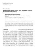
Figure 1 shows the comparison of upper a nd lower
bounds, approximation and exact interference power for the
AFT-MC system without the GI. The channel is modeled by
classical Jakes Doppler Power Profile (DPP) and rural area
(RA) multipath line-of sight (LOS) environment with an
exponential Power Delay Profile (PDP) as defined in COST
207 [10]. The AFT-MC and channel parameters are c
0
=
356 Hz, c
1
=−8.5 · 10
8
Hz
2
, ν
d
= 517 Hz, ν

LOS
= 0.7ν
d
, K =
15 dB, τ
max
= 0.7 μs, and T ∈ [10 μs, 2 ms]. From Figure 1,
4 EURASIP Journal on Wireless Communications and Networking
Pint (dB)
Interference power
0.50 1 1.5 2 2.5 3 3.5 4 4.5
−40
−35
−30
−25
−20
−15
−10
Upper bound
Lower bound
Approximated
Exact
(ν
d
+ |c
0
| +2|c
1
|τ
max

)T
Figure 1: Comparison of the upper and lower bound, approx-
imated and exact interference power for the AFT-MC system
without the GI.
it can be seen that the upper and lower bounds are close only
for (ν
d
+|c
0
| +2|c
1
|τ
max
)T<0.25, whereas the approximated
interference power stays close to the exact interference power
in the whole range (difference is around 1 dB, when (ν
d
+
|c
0
| +2|c
1
|τ
max
)T>1).
Note that if sufficient GI is inserted, effects of multipath
delays are eliminated and the approximation of interference
power simplifies to [2]
P
I

∼
=
(
1/
(
K +1
))
P
UB
ICI
1/
(
K +1
)
+ P
UB
ICI
. (17)
3. Optimal Parameters
3.1. Channel Models. Multipath scenario with LOS compo-
nent represents a general channel model in aeronautical and
LMS communications. We assume that the LOS component
with power K/(K + 1) arrives at τ
= 0withfrequencyoffset
ν
LOS
. Multipath components are modeled by the scattering
function S
diff
(τ, ν)withpower1/(K +1).

A general scattering function can be defined as
S
(
τ, ν
)
=
K
K +1
δ
(
τ
)
δ
(
ν
− ν
LOS
)
+
1
K +1
S
diff
(
τ, ν
)
.
(18)
Analysis of channel behavior depends on the S
diff

(τ, ν)
properties. There are three characteristic cases:
(1) multipath scenario with LOS component and separa-
ble scattering function,
(2) multipath scenario with LOS component and cluster
of scattered paths,
(3) multipath scenario with two-paths.
For each of special cases, the optimal par ameters for the
AFT-MC system and interference power can be calculated in
the closed form.
Optimal parameters c
0opt
and c
1opt
can be obtained as
[11]
c
0opt
=
m
02
(
0, 0
)
m
10
(
0, 0
)
− m

01
(
0, 0
)
m
11
(
0, 0
)
m
02
(
0, 0
)
− m
2
01
(
0, 0
)
,
c
1opt
=
m
11
(
0, 0
)
− m

01
(
0, 0
)
m
10
(
0, 0
)
2

m
02
(
0, 0
)
− m
2
01
(
0, 0
)

.
(19)
Moments m
20
(0, 0) and m
02
(0, 0) represent the Doppler

spread ν
m
and delay spread τ
m
of the channel in the OFDM
system, respectively. Moments m
10
(0, 0) and m
01
(0, 0) quan-
tify the average Doppler shift ν
e
and delay shift τ
e
,respec-
tively. In typical wireless scenario, the scattering function
S(τ, ν) can be decomposed via the PDP Q(τ) and DPP
P(ν)andm
11
(0, 0) can be calculated using m
01
(0, 0) and
m
10
(0, 0). Thus, the AFT parameters in real-life environment
can be calculated using estimations of the Doppler and delay
spreads and average shifts.
3.1.1. Multipath Scenario with LOS Component and Separable
Scattering Function. Consider the case that S
diff

(τ, ν)is
separable, that is,
S
(
τ, ν
)
=
K
K +1
δ
(
τ
)
δ
(
ν
− ν
LOS
)
+
1
K +1
Q
diff
(
τ
)
P
diff
(

ν
)
,
(20)
where Q
diff
(τ)andP
diff
(ν) denote the PDP and DPP of
the scattered components, respectively. Furthermore, assume
that

ν
d
−ν
d
P
diff
(ν)dν = 1and

τ
diff
0
Q
diff
(τ)dτ = 1, where ν
d
denotes the maximal Doppler shift and τ
diff
represents the

maximal excess delay. Now, α
i
and β
j
can be defined as
α
i
=

ν
d
−ν
d
P
diff
(
ν
)
ν
i
dν,
β
j
=

τ
diff
0
Q
diff

(
τ
)
τ
j
dτ,
(21)
respectively. The optimal parameters c
0opt
and c
1opt
can be
expressed as
c
0opt
=
(
K/
(
K +1
))
ν
LOS
β
2
+
(
1/
(
K +1

))
α
1

β
2
− β
2
1

β
2
−
(
1/
(
K +1
))
β
2
1
,
c
1opt
=
1
2
K
K +1
α

1
β
1
− ν
LOS
β
1
β
2
−
(
1/
(
K +1
))
β
2
1
.
(22)
3.1.2. Multipath Scenar io with LOS Component and Cluster
of Scattered Paths. In the multipath channel with LOS
component a nd cluster of scattered paths, the scattering
function takes form
S
(
τ, ν
)
=
K

K +1
δ
(
τ
)
δ
(
ν
− ν
LOS
)
+
1
K +1
δ
(
τ
− τ
diff
)
P
diff
(
ν
)
.
(23)
EURASIP Journal on Wireless Communications and Networking 5
For these channels, the optimal parameters c
0opt

and c
1opt
are
c
0opt
= ν
LOS
,
c
1opt
=
1
2
α
1
− ν
LOS
τ
diff
.
(24)
3.1.3. Multipath Scenario with Two Paths. Often the signal
propagates over the two paths, one direct and one reflected.
The channel model is further simplified with the scattering
function that has nonzero values only in two points (0, ν
LOS
)
and (τ
diff
, ν

diff
), that is,
S
(
τ, ν
)
=
K
K +1
δ
(
τ
)
δ
(
ν
− ν
LOS
)
+
1
K +1
δ
(
τ
− τ
diff
)
δ
(

ν
− ν
diff
)
.
(25)
Now, the optimal parameters c
0opt
and c
1opt
reduce to
c
0opt
= ν
LOS
,
c
1opt
=
1
2
ν
diff
− ν
LOS
τ
diff
.
(26)
In the two-path channel, m

20
(c
0
, c
1
), with the optimal
parameters, equals 0. Since the interference power depends
on m
20
(c
0
, c
1
), it is obvious that P
I
= 0 in the AFT-
MC system. It is shown in [3] that the two-path channel
represents the worst case for OFDM since the interference
equals the upper bound P
I
= (1/3)ν
2
LOS
π
2
T
2
. On the other
hand, two-path channel represents the best case scenario
for the AFT-MC system, since the interference is completely

removed.
3.2. Synchronization in the AFT-MC Systems. The optimal
parameters are also related to the time and frequency
synchronization. The time and frequency offsets may occur
in case of time delay caused by the multipath and nonideal
time synchronization, sampling clock frequency discrepancy,
carrier frequency offset (CFO) induced by the Doppler
effects or poor oscillator alignments [12]. The problem
of time and frequency synchronization has been widely
studiedinOFDM[13–17]. The effects of time delays can
be efficiently evaded by using the GI. If the length of the
GI exceeds that of the channel impulse response, there will
be no time offset and signal will be perfectly reconstructed.
The same approach can be used in the AFT-MC system, since
the GI is used in the same manner as in OFDM. Similarly,
the frequency offset correction, defined by the parameter
c
0
, is u sed in both the AFT-MC and OFDM system.
Thus, the offset correction techniques identified for OFDM
can be employed in the AFT-MC system. The AFT-MC
system, however, also depends on the frequency parameter
c
1
. The effects of estimation errors can be modeled by
using parameter m
20
(c
0
, c

1
), which represents the equivalent
Doppler spread ν
m
(c
0
, c
1
)
ν
m
(
c
0
, c
1
)
=

ν
d
−ν
d

τ
max
0
S
(
τ, ν

)
×
(
ν
− c
0
− ε
0
− 2
(
c
1
+ ε
1
)
τ
)
2
dτ dν,
(27)
Interference power
−90
−80
−70
−60
−50
−40
−30
−20
−100

Pint (dB)
−100 −50 0 50 100
c
1
error (%)
AFT-MC
OFDM
LMS
Aeronautical
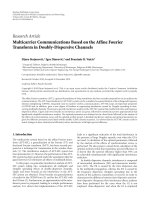
Figure 2: Comparison of the effects of c
1
estimation errors on
the interference power in the AFT-MC and OFDM system in
aeronautical and LMS channels.
where ε
0
and ε
1
represent errors i n estimation of c
0
and c
1
,
respectively. Since the CFO is the same in the OFDM and
AFT-MC system, ε
0
affects the properties of both systems
to the similar extent. However, ε
1
affects only the AFT-MC

system and it reduces the interference suppression ability of
the system.
Inserting c
0
+ε
0
and c
1
+ε
1
in (27), after some calculation,
the difference between Doppler spread in the system with and
without estimation errors can be expressed as
Δν
m
(
c
0
, c
1
)
= ε
2
0
− 2ε
0
m
10
(
0, 0

)
− 4ε
0
ε
1
m
01
(
0, 0
)
+4ε
2
1
m
02
(
0, 0
)
+2ε
1
m
11
(
0, 0
)
.
(28)
In case that c
1
estimation error is equal to zero, the

difference between Doppler spread Δν
m
(c
0
, 0) represents an
CFO and it depends on m
10
and ε
0
.However,ifc
0
estimation
error is equal to zero, the difference between Doppler spreads
Δν
m
(c
0
,0) represents an offset specific for the AFT-MC
system and it depends on m
01
, m
02
, m
11
,andε
1
.
The effects of parameter c
1
estimation errors in aeronau-

tical and LMS channels for v
= 20 m/s are illustrated in
Figure 2. The error is expressed as ε
1
/c
1
.Itcanbeobserved
that in case of estimation error of 100%, the AFT-MC
system has the same properties as the OFDM, whereas
for smaller errors the AFT-MC system performs better.
Therefore, even if significant estimation error is present,
the AFT-MC system is better in interference reduction than
the OFDM. This robustness gives a possibility to use the
AFT-MC system in the channels where parameters cannot
be perfectly obtained. In each presented example, even for
20% error, the interference power in the AFT-MC system in
presented examples is still bellow
−40 dB.
6 EURASIP Journal on Wireless Communications and Networking
3.3. Spectral Efficiency Maximization. The multicarrier com-
munication system is expected to be able to efficiently use
the available spectrum and combat interference. The symbol
is typically preceded by the GI whose duration is longer than
the delay spread of the propagation channel. Adding the GI
the ISI can be completely eliminated. Although the GI is an
elegant solution to cope with the distortions of the multipath
channel, it reduces the bandwidth efficiency, which signifi-
cantly affects the channel utilization. T he spectral efficiency
can be defined as
η

=
T
T + T
CP
=
1
1+G
,
(29)
where G
= T
CP
/T defines the ratio between the symbol and
GI durations. This is also a measure of the bit rate reduction
requiredbytheGI.Hence,smallerG leads to the higher
bit rate. In the OFDM case, to mitigate effects of multipath
propagation, the length of the GI has to be chosen as a
small frac tion of the OFDM symbol length. However, if the
OFDM symbol length is long, the ICI caused by the Doppler
spreading significantly derogates the system performance.
Nevertheless, in the AFT-MC system, the Doppler spreading
in time-varying multipath channels is mitigated by the
chirp modulation properties, and therefore it is possible to
significantly increase the symbol period and maximize η.The
AFT-MC system with the GI can reduce interference power,
but its spectral efficiency is highly dependable on the symbol
period.Theoptimalsymbolperiodisatradeoff between
reducing interference to the targeted level and maximizing
the spectral efficiency. Inserting (9) into (17), the optimal
symbol period can be obtained as

T
opt
=

3P
I
m
20
(
c
0
, c
1
)
π
2
(
1
− P
I
(
K +1
))
.
(30)
The optimal symbol period, for any predefined P
I
,can
be directly calculated based on the channel parameters
m

20
(c
0
, c
1
)andK. The corresponding spectral efficiency η
can be easily calculated inserting (30) into (29). Now, for
predefined P
I
, the corresponding spectral efficiency can be
also directly calculated.
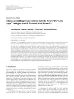
The dependence between the spectral efficiency and
interference power in aeronautical en-route and LMS chan-
nels with the LOS and scattered multipath components is
shown in Figure 3. It can be seen that in each scenario, for the
spectral efficiency η
= 95%, the interference power is bellow
−40 dB. Therefore, use of the GI interval with the optimal T
does not significantly reduce spectral efficiency.
4. Practical Implementation
4.1. AFT-MC in Aeronautical Channels. The aeronautical
channel represents a challenging setup for the multicar rier
systems. Four different channel scenarios can be defined: en-
route, arrival and takeoff, taxi, and parking scenario [18].
These scenarios are characterized by different types of fading,
Doppler spreads, and delays. In the parking scenario, only
multipath components exist, whereas in all other scenarios
there is in addition a strong LOS component. In all scenarios,
−90
−80

−70
−60
−50
−40
−30
−10
−20
0
Pint (dB)
90 92 94 96 98 100
Spectral efficiency η (%)
Interference power
Aeronautical
LMS
AFT-MC
OFDM
Figure 3: Comparison of the interference power for different
spectral efficiency in aeronautical and LMS channels with the LOS
and scattered multipath components.
we take the carrier frequency f
c
= 1.55 GHz (corresponding
to the L band), and the maximum Doppler shift depends on
the velocity of the aircraft ν
d
= v
max
f
c
/c,wherec denotes the

speed of light. Other channel parameters are taken from [18].
All interferences powers have been calculated using (16)and
(17).
4.1.1. En-Route Scenario. The en-route scenario describes
ground-to-air or air-to-air communications when the air-
craft is airborne. This multipath channel characterizes a LOS
path and cluster of scattered paths. Typical maximal speeds
are v
max
= 440 m/s for ground-air links and v
max
= 620 m/s
for air-air links. In this scenario, the scattered components
are not uniformly distributed in the interval [0, 2π) leading
to the asymmetrical DPP. Actually, the beamwidth of the
scattered components is reported to be Δϕ
B
= 3.5
◦
[18].
Maximal excess delay equals τ
diff
= 66 μs, and Rician factor is
K
= 15 dB. In this case, S(τ, ν)takesform(23). The DPP can
be modeled by the restric ted Jakes model [19]
P
diff
(
ν

)
= ψ
1
ν
d

1 −
(
ν/ν
d
)
2
, ν
1
≤ ν ≤ ν
2
,
(31)
and ψ
= 1/(arcsin(ν
2
/ν
d
) − arcsin(ν
1
/ν
d
)) denotes a factor
introduced to normalize the DPP.
Consider the worst case when the LOS component

comes directly to the front of the aircraft and scattered
components come from behind. Now, ν
1
=−ν
d
and ν
2
=
−
ν
d
(1 − Δϕ
B
/π), where Δϕ
B
represents the beamwidth of
the scattered components symmetrically distributed around
ϕ
= π.
EURASIP Journal on Wireless Communications and Networking 7
For this model, parameters m
0 j
(0, 0) for j ∈ N can be
calculated as
m
0 j
(
0, 0
)
=

1
K +1
τ
j
diff
.
(32)
Moments m
i0
(0, 0) can be directly calculated from (13).
The first two moments can be obtained as
m
10
(
0, 0
)
=
K
K +1
ν
LOS
+
1
K +1
ψ


ν
2
d

− ν
2
1
−

ν
2
d
− ν
2
2

,
(33)
m
20
(
0, 0
)
=
K
K +1
ν
2
LOS
+
1
K +1
ψ
2

×

ν
1

ν
2
d
− ν
2
1
− ν
2

ν
2
d
− ν
2
2

+
1
2
ν
2
d
K +1
.
(34)

Now, parameters m
ij
(0, 0) for i>0andj>0canbe
recursively calculated as
m
ij
(
0, 0
)
= m
0 j
(
0, 0
)(
K +1
)

m
i0
(
0, 0
)
−
K
K +1
ν
i
LOS

.

(35)
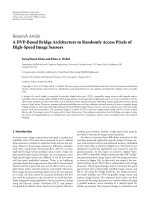
Figure 4 illustrates the comparison of the interference
power obtained for the OFDM and AFT-MC system with
and without the GI in the en-route scenario for different
T and aircraft velocity v
= 400 m/s. From Figure 4 it
can be observed that even without the GI, the AFT-MC
system is significantly better in suppressing the interference
in comparison to the OFDM with the GI. In the AFT-MC
system, the ICI is significantly reduced by the properties
of the system and larger T can be implemented in order
to combat ISI. Thus, in the en-route scenario, AFT-MC
significantly suppresses the total interference power. In case
that the GI is used, even better interference reduction can
be achieved with slightly lower spectral efficiency. It can be
observed that the interference power for the AFT-MC system
with the GI even for the extremely high aircraft velocity of
v
= 400 m/s can be below −40 dB. Note that even without
the GI interference power below
−28 dB can be achieved.
4.1.2. Arrival and Takeoff Scenario. Thearrivalandtake-
off scenario models communications between ground and
aircraft when the aircraft takeoffsorisabouttoland.It
is assumed that the LOS and scattered components arrive
directly in front of the aircraft and the beamwidth of the
scattered components from the obstacles in the airport is
180
◦
. The maximal speed of the aircraft is 150 m/s, and the

Rician factor K
= 15 dB. In this channel, S(τ, ν)takesform
(20). The PDP can be modeled as an exponential function
similarly to the rural nonhilly COST 207 model [10]
Q
diff
(
τ
)
=
⎧
⎨
⎩
c
n
e
−t/τ
s
if 0 ≤ τ<τ
diff
,
0, elsewhere,
(36)
where τ
diff
denotes the maximal excess delay, τ
s
characterizes
the slope of the function, and
c

n
=
1
τ
s
(
1
− e
−τ
diff
/τ
s
)
(37)
1234
5
678
9
10
×10
−3
−70
−60
−50
−40
−30
−20
−10
T
Pint (dB)

Interference power
AFT-MC without GI
AFT-MC with GI
OFDM without GI
OFDM with GI
Figure 4: Comparison of the interference power in the en-route
scenario for the AFT-MC and OFDM system.
represents the normalization factor. For the rural nonhilly
model, τ
diff
= 0.7 μsandτ
s
= 1/9.2 μs.
The DPP can be modeled by the restricted Jakes model
(31), with ν
1
= 0andν
2
= ν
d
. Parameters m
10
(0, 0) and
m
20
(0, 0) can be obtained by inserting ν
1
and ν
2
into (33)

and (34), respectively.
Parameters m
0 j
(0, 0) for j ∈ N can be calculated
recursively as
m
0 j
(
0, 0
)
= m
0 j−1
(
0, 0
)
jτ
s
−
1
K +1
c
n
τ
s
e
−τ
diff
/τ
s
τ

j
diff
,
(38)
where m
01
(0, 0) = (1/(K +1))c
n
τ
s
(τ
s
− e
−τ
diff
/τ
s
(τ
diff
+ τ
s
)).
Moments m
ij
(0, 0) can be calculated from (35).
Figure 5 shows the comparison of the interference power
in the OFDM and AFT-MC system with and without
the GI in the arrival and takeoff scenario for different T
and aircraft velocity v
= 100 m/s. The AFT-MC system

still outperforms the OFDM, since the beamwidth of the
multipath component is 180
◦
. Similarly to the prev ious case,
introduction of the GI efficiently combats the interference for
shorter symbol periods.
4.1.3. Taxi Scenario. The taxi scenario is a model for
communications when the aircraft is on the ground and
approaching or moving away from the terminal. The LOS
path comes from the front, but not directly, resulting in
smaller Doppler shifts, in this example ν
LOS
= 0.7ν
d
.The
maximal speed is 15 m/s, the Rician factor K
= 6.9dB,and
the reflected paths come uniformly, resulting in the classical
Jakes DPP (31), with ν
1
=−ν
d
and ν
2
= ν
d
. Inserting ν
1
and
ν

2
into (33)and(34) parameters m
10
(0, 0) and m
20
(0, 0) can
be, respectively, calculated.
The PDP can be modeled similarly to the rural (nonhilly)
COST 207 model by the exponential function (36) with the
8 EURASIP Journal on Wireless Communications and Networking
1234
5
678
9
10
×10
−4
T
Pint (dB)
Interference power
AFT-MC without GI
AFT-MC with GI
OFDM without GI
OFDM with GI
−70
−65
−60
−55
−50
−45

−40
−35
−30
−25
−20
Figure 5: Comparison of the interference power in the arrival and
takeoff scenario for the AFT-MC and OFDM system.
maximal excess delay of τ
diff
= 0.7 μsandτ
s
= 1/9.2 μs.
Moments m
ij
(0, 0) can be calculated from (35).
The comparison of the interference power in the OFDM
and AFT-MC systems with and without the GI, in the
taxi scenario for different T and aircraft velocity v
=
10 m/s is shown in Figure 6. Since the PDP has exponential
profile and the beamwidth of the multipath component is
360
◦
, interference characteristics of the OFDM and AFT-
MC system are closer comparing to the previous example.
However, it can been observed that the interference power in
the AFT-MC system is still lower than in the OFDM, since the
AFT-MC system exploits the existence of LOS component.
4.1.4. Parking Scenario. The parking scenario models the
arrival of the aircraft to the terminal or parking. The LOS

path is blocked, resulting in Rayleigh fading. The maximal
speed of the aircraft is 5.5 m/s, and the DPP can be modeled
as the classical Jakes profile (31)withν
1
=−ν
d
and ν
2
= ν
d
.
The parking scenario is similar to the typical urban COST
207 model, with the exponential PDP (36), τ
diff
= 7 μs, and
slope time τ
s
= 1 μs[10].
Figure 7 shows the comparison of the interference power
in the OFDM and AFT-MC system with and without the GI
in the parking scenario for different T and aircraft velocity
v
= 2.5 m/s. Since there is no LOS and DPP is symmetrical,
the AFT-MC system reduces to the ordinary OFDM (c
0
=
0). Thus, there is no difference in characteristics between the
MC-AFT and OFDM.
4.2. AFT-MC in Land-Mobile Satellite Channels. The LMS
channel represents another example of environment with

strong LOS component and scattered multipath compo-
nents. We will discuss different cases of Land-Mobile Low
Earth Or bit (LEO) satellite channels. In the following
1234
5
678
9
10
×10
−4
−70
−60
−50
−40
−30
−20
T
Pint (dB)
Interference power
AFT-MC without GI
AFT-MC with GI
OFDM without GI
OFDM with GI
−80
Figure 6: Comparison of the interference power in the taxi scenario
fortheAFT-MCandOFDMsystem.
×10
−3
−70
−60

−50
−40
−30
−20
−10
T
Pint (dB)
Interference power
AFT-MC without GI
AFT-MC with GI
OFDM without GI
OFDM with GI
0.5 1 1.5 2 2.5 3 3.5 4 4.5 5
Figure 7: Comparison of the interference power in the parking
scenario for the AFT-MC and OFDM system.
examples, it is assumed that carrier frequency f
c
= 1.55 GHz,
Rician factor K
= 7 dB, and the maximal velocity is up
to v
max
= 50 m/s. In each example, the AFT-MC system
is compared to the OFDM with the offset correction. The
interference powers are calculated using (16)and(17).
Consider the LMS channel, where a mobile terminal uses
a narrow-beam antenna (e.g., digital beamforming (DBF)
antenna) to track and communicate with satellite. Note that
in case where a directive antenna is employed at the user ter-
minal, the classical Jakes model is no longer applicable [20].

EURASIP Journal on Wireless Communications and Networking 9
0 0.2 0.4 0.6 0.8 1
×10
−3
−250
−200
−150
−100
−50
0
T
Pint (dB)
Interference power
AFT-MC without GI
AFT-MC with GI
OFDM without GI
OFDM with GI
Figure 8: Comparison of the AFT-MC and OFDM interference
power in the two-path LMS channel.
4.2.1. Two-Path. Let us first consider the two-path channel
model, with ν
diff
=−ν
d
, ν
LOS
= ν
d
,andτ
diff

= 0.7 μs.
The channel is characterized by the scattering function g iven
in (25), whereas the optimal parameters can be calculated
from (26). Figure 8 compares the interference power for
the OFDM and AFT-MC systems. It is obvious that the
AFT-MC system completely eliminates interference, whereas
interference in OFDM has significant value. Thus, in the two-
path LMS channels, the AFT-MC system is the optimal one.
4.2.2. LOS and Scattered Multipath Components. Consider
the channel model with LOS and scattered multipath compo-
nents that arrives at the receiver at τ
diff
= 33 μs. The channel
is characterized by the scattering function given in (23),
whereas DPP can be modeled by the asymmetrical restricted
Jakes model (31). Note that this case DPP is similar to the
en-route scenario in aeronautical channels. However, in this
example, the arrival angles of the multipath components are
uniformly distributed, but the antenna is narrow-beam. Let
us assume that the angle between the direction of travel and
the antenna bearing angle is η
= 15
◦
, the elevation angle
of the satellite transmitter relative to the mobile receiver is
ξ
= 45
◦
, and the antenna beamwidth is β = 12
◦

.Here,
ν
1
= ν
d
cos(η + β/2), ν
2
= ν
d
cos(η − β/2), and ν
LOS
=
ν
d
cos(ξ)cos(η)[21].
Figure 9 compares the interference power for the OFDM
and AFT-MC systems. It can be observed that the AFT-MC
system clearly outperforms OFDM. Thus, the implemen-
tation of the AFT-MC system in the LMS channels with
LOS path and scattered multipath components leads to the
significant reduction of interference.
4.2.3. LOS and Expone ntial Multipath Components. This
channel is described by the scattering functions given in
0
0.002
0.004 0.006 0.008 0.01
−90
−80
−70
−60

−50
−40
−30
−20
−10
0
T
Pint (dB)
Interference power
AFT-MC without GI
AFT-MC with GI
OFDM without GI
OFDM with GI
Figure 9: Comparison of the AFT-MC and OFDM interference
power in the LMS channel with LOS component and cluster of
scattered paths.
0 0.2 0.4 0.6 0.8 1
×10
−3
T
Interference power
AFT-MC without GI
AFT-MC with GI
OFDM without GI
OFDM with GI
−90
−80
−70
−60
−50

−40
−30
−20
−10
−100
Pint (dB)
Figure 10: Comparison of the AFT-MC and OFDM interference
power in the LMS channel with LOS component and COST 207
multipath model.
(20). Assume that the mobile terminal is out of urban
areas, and PDP can be modeled as an exponential function
similarly to the rural nonhilly COST 207 model (36). The
DPP is asy mmetrical and it can be modeled by the restric ted
Jakes model (31). Figure 10 shows the comparison of the
interference power in the OFDM and AFT-MC systems in the
LMS scenario with narrow-beam antenna. It can be observed
that the AFT-MC system outperforms the OFDM when the
narrow-beam antenna is used.
10 EURASIP Journal on Wireless Communications and Networking
5. Conclusion
In this paper, we present performance analysis of the AFT-
MC systems in doubly dispersive channels with focus on
aeronautical and LMS channels. The upper and lower
bounds on interference power are given, followed by an
approximation of the interference power, based on the mod-
ified upper bound, that significantly simplify calculation.
The optimal parameters are obtained in a closed form, and
practical examples for their calculation are given.
Since the AFT-MC system can be considered as a
generalization of the OFDM, it is applicable in all chan-

nels where the OFDM is used with, at least, the same
performance. Additional improvements, due to resilience
to the interference in time-varying wireless channels w ith
significant Doppler spread and LOS component, offer new
possibilities in designing multicarrier systems for aeronau-
tical and LMS communications. It has been shown that the
spectral efficiency higher than 95% can be a chieved, with an
acceptable level of interference.
References
[1] T. Erseghe, N. Laurenti, and V. Cellini, “A multicarrier
architecture based upon the affine fourier transform,” IEEE
Transactions on Communications, vol. 53, no. 5, pp. 853–862,
2005.
[2] D. Stojanovi
´
c, I. Djurovi
´
c, and B. R. Vojcic, “Interference
analysis of multicarrier systems based on affine fourier
transform,” IEEE Transactions on Wireless Communications,
vol. 8, no. 6, pp. 2877–2880, 2009.
[3] Y. Li and L. J. Cimini, “Bounds on the interchannel
interference of OFDM in time-varying impairments,” IEEE
Transactions on Communications, vol. 49, no. 3, pp. 401–404,
2001.
[4] T. Gilbert, J. Jin, J. Berger, and S. Henriksen, “Future aeronau-
tical communication infrastructure technology investigation,”
Tech. Rep. NASA/CR-2008-215144, NASA, Los Angeles, Calif,
USA, April 2008.
[5] W. W Wu, “Satellite communications,” Proceedings of the IEEE,

vol. 85, no. 6, pp. 998–1010, 1997.
[6] J. V. Evans, “Satellite systems for personal communications,”
Proceedings of the IEEE, vol. 86, no. 7, pp. 1325–1340, 1998.
[7] P. A. Bello, “Characterization of randomly time-variant linear
channels,” IEEE Transactions on Communications Systems, vol.
11, no. 4, pp. 360–393, 1963.
[8] M. Abramowitz and I. A. Stegun, Handbook of Mathematical
Functions, Dover, New York, NY, USA, 1964.
[9]J.G.Proakis,Digital Communications, McGraw-Hill, New
York, NY, USA, 4th edition, 2000.
[10] M. Falli, Ed., “Digital land mobile radio communications-
COST 207: final report,” Tech. Rep., Commission of European
Communities, Luxembourg, Germany, 1989.
[11] S. Barbarossa and R. Torti, “Chirped-OFDM for transmis-
sions over time-varying channels with linear delay/Doppler
spreading,” in Proceedings of the IEEE Interntional Conference
on Acoustics, Speech, and Signal Processing (ICASSP ’01),pp.
2377–2380, Salt Lake City, Utah, USA, May 2001.
[12] D. Huang and K. B. Letaief, “An interference-cancellation
scheme for carrier frequency offsets correction in OFDMA
systems,” IEEE Transactions on Communications, vol. 53, no.
7, pp. 1155–1165, 2005.
[13] P. H. Moose, “Technique for orthogonal frequency division
multiplexing frequency offset correction,” IEEE Transactions
on Communications, vol. 42, no. 10, pp. 2908–2914, 1994.
[14] T. Pollet and M. Moeneclaey, “Synchronizability of OFDM
signals,” in Proceedings of the IEEE Global Telecommunica-
tions Conference (Globecom ’95), pp. 2054–2058, Singapore,
November 1995.
[15] J. J. van de Beek, M. Sandell, and P. O. B

¨
orjesson, “ML
estimation of time and frequency offset in OFDM systems,”
IEEE Transactions on Signal Processing, vol. 45, no. 7, pp. 1800–
1805, 1997.
[16] T. M. Schmidl and D. C. Cox, “Robust frequency and
timing synchronization for OFDM,” IEEE Transactions on
Communications, vol. 45, no. 12, pp. 1613–1621, 1997.
[17] B. Yang, K. B. Letaief, R. S. Cheng, and Z. Cao, “Timing
recovery for OFDM transmission,” IEEE Journal on Selected
Areas in Communications, vol. 18, no. 11, pp. 2278–2291, 2000.
[18] E. Haas, “Aeronautical channel modeling,” IEEE Transactions
on Vehicular Technology
, vol. 51, no. 2, pp. 254–264, 2002.
[19] M. Paetzold, Mobile Fading Channels, John Wiley & Sons, New
York, NY, USA, 2002.
[20] C. Kasparis, P. King, and B. G. Evans, “Doppler spectrum of
the multipath fading channel in mobile satellite systems with
directional terminal antennas,” IET Communications, vol. 1,
no. 6, pp. 1089–1094, 2007.
[21] M. Rice and E. Perrins, “A simple figure of merit for evaluating
interleaver depth for the land-mobile satellite channel,” IEEE
Transactions on Communications, vol. 49, no. 8, pp. 1343–
1353, 2001.