Essentials of Control Techniques and Theory_1 pptx

Essentials of
Control Techniques
and Theory
91239.indb 1 10/12/09 1:40:29 PM
This page intentionally left blank
Essentials of
Control Techniques
and Theory
John Billingsley
91239.indb 3 10/12/09 1:40:30 PM
CRC Press
Taylor & Francis Group
6000 Broken Sound Parkway NW, Suite 300
Boca Raton, FL 33487-2742
© 2010 by Taylor and Francis Group, LLC
CRC Press is an imprint of Taylor & Francis Group, an Informa business
No claim to original U.S. Government works
Printed in the United States of America on acid-free paper
10 9 8 7 6 5 4 3 2 1
International Standard Book Number: 978-1-4200-9123-6 (Hardback)
This book contains information obtained from authentic and highly regarded sources. Reasonable efforts
have been made to publish reliable data and information, but the author and publisher cannot assume
responsibility for the validity of all materials or the consequences of their use. The authors and publishers
have attempted to trace the copyright holders of all material reproduced in this publication and apologize to
copyright holders if permission to publish in this form has not been obtained. If any copyright material has
not been acknowledged please write and let us know so we may rectify in any future reprint.
Except as permitted under U.S. Copyright Law, no part of this book may be reprinted, reproduced, transmit-
ted, or utilized in any form by any electronic, mechanical, or other means, now known or hereafter invented,
including photocopying, microfilming, and recording, or in any information storage or retrieval system,
without written permission from the publishers.

For permission to photocopy or use material electronically from this work, please access www.copyright.
com ( or contact the Copyright Clearance Center, Inc. (CCC), 222 Rosewood
Drive, Danvers, MA 01923, 978-750-8400. CCC is a not-for-profit organization that provides licenses and
registration for a variety of users. For organizations that have been granted a photocopy license by the CCC,
a separate system of payment has been arranged.
Trademark Notice: Product or corporate names may be trademarks or registered trademarks, and are used
only for identification and explanation without intent to infringe.
Library of Congress Cataloging-in-Publication Data
Billingsley, J. (John)
Essentials of control techniques and theory / John Billingsley.
p. cm.
Includes index.
ISBN 978-1-4200-9123-6 (hardcover : alk. paper)
1. Automatic control. 2. Control theory. I. Title.
TJ223.M53B544 2010
629.8 dc22 2009034834
Visit the Taylor & Francis Web site at

and the CRC Press Web site at

91239.indb 4 10/12/09 1:40:30 PM
v
Contents
Preface xi
Author xiii
ISECTION ESSENTIALS OF CONTROL TECHNIQUES—
WHAT YOU NEED TO KNOW
1 Introduction: Control in a Nutshell; History, Theory, Art, and
Practice 3
1.1 e Origins of Control 3

1.2 Early Days of Feedback 5
1.3 e Origins of Simulation 6
1.4 Discrete Time 7
2 Modeling Time 9
2.1 Introduction 9
2.2 A Simple System 9
2.3 Simulation 11
2.4 Choosing a Computing Platform 12
2.5 An Alternative Platform 15
2.6 Solving the First Order Equation 16
2.7 A Second Order Problem 19
2.8 Matrix State Equations 23
2.9 Analog Simulation 24
2.10 Closed Loop Equations 26
3 Simulation with JOLLIES: JavaScript On-Line Learning
Interactive Environment for Simulation 29
3.1 Introduction 29
3.2 How a JOLLIES Simulation Is Made Up 31
3.3 Moving Images without an Applet 35
3.4 A Generic Simulation 38
91239.indb 5 10/12/09 1:40:31 PM
vi ◾ Contents
4 Practical Control Systems 41
4.1 Introduction 41
4.2 e Nature of Sensors 42
4.3 Velocity and Acceleration 44
4.4 Output Transducers 44
4.5 A Control Experiment 46
5 Adding Control 49
5.1 Introduction 49

5.2 Vector State Equations 49
5.3 Feedback 52
5.4 Another Approach 53
5.5 A Change of Variables 55
5.6 Systems with Time Delay and the PID Controller 57
5.7 Simulating the Water Heater Experiment 60
6 Systems with Real Components and Saturating
Signals—Use of the Phase Plane 63
6.1 An Early Glimpse of Pole Assignment 63
6.2 e Effect of Saturation 65
6.3 Meet the Phase Plane 65
6.4 Phase Plane for Saturating Drive 70
6.5 Bang–Bang Control and Sliding Mode 74
7 Frequency Domain Methods 77
7.1 Introduction 77
7.2 Sine-Wave Fundamentals 78
7.3 Complex Amplitudes 79
7.4 More Complex Still-Complex Frequencies 81
7.5 Eigenfunctions and Gain 81
7.6 A Surfeit of Feedback 83
7.7 Poles and Polynomials 85
7.8 Complex Manipulations 87
7.9 Decibels and Octaves 88
7.10 Frequency Plots and Compensators 89
7.11 Second Order Responses 92
7.12 Excited Poles 93
8 Discrete Time Systems and Computer Control 97
8.1 Introduction 97
8.2 State Transition 98
8.3 Discrete Time State Equations and Feedback 101

8.4 Solving Discrete Time Equations 102
8.5 Matrices and Eigenvectors 103
8.6 Eigenvalues and Continuous Time Equations 104
91239.indb 6 10/12/09 1:40:32 PM
Contents ◾ vii
8.7 Simulation of a Discrete Time System 105
8.8 A Practical Example of Discrete Time Control 107
8.9 And ere’s More 110
8.10 Controllers with Added Dynamics 112
9 Controlling an Inverted Pendulum 115
9.1 Deriving the State Equations 115
9.2 Simulating the Pendulum 119
9.3 Adding Reality 122
9.4 A Better Choice of Poles 123
9.5 Increasing the Realism 124
9.6 Tuning the Feedback Pragmatically 126
9.7 Constrained Demand 127
9.8 In Conclusion 129
ISECTION I ESSENTIALS OF CONTROL THEORY—WHAT
YOU OUGHT TO KNOW
10 More Frequency Domain Background Theory 133
10.1 Introduction 133
10.2 Complex Planes and Mappings 134
10.3 e Cauchy–Riemann Equations 135
10.4 Complex Integration 138
10.5 Differential Equations and the Laplace Transform 140
10.6 e Fourier Transform 144
11 More Frequency Domain Methods 147
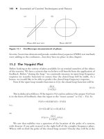
11.1 Introduction 147
11.2 e Nyquist Plot 148

11.3 Nyquist with M-Circles 151
11.4 Software for Computing the Diagrams 153
11.5 e “Curly Squares” Plot 154
11.6 Completing the Mapping 155
11.7 Nyquist Summary 156
11.8 e Nichols Chart 156
11.9 e Inverse-Nyquist Diagram 158
11.10 Summary of Experimental Methods 162
12 The Root Locus 165
12.1 Introduction 165
12.2 Root Locus and Mappings 165
12.3 A Root Locus Plot 169
12.4 Plotting with Poles and Zeroes 172
12.5 Poles and Polynomials 173
91239.indb 7 10/12/09 1:40:32 PM
viii ◾ Contents
12.6 Compensators and Other Examples 176
12.7 Conclusions 178
13 Fashionable Topics in Control 181
13.1 Introduction 181
13.2 Adaptive Control 182
13.3 Optimal Control 182
13.4 Bang–Bang, Variable Structure, and Fuzzy Control 182
13.5 Neural Nets 184
13.6 Heuristic and Genetic Algorithms 184
13.7 Robust Control and H-infinity 185
13.8 e Describing Function 185
13.9 Lyapunov Methods 186
13.10 Conclusion 187
14 Linking the Time and Frequency Domains 189

14.1 Introduction 189
14.2 State-Space and Transfer Functions 189
14.3 Deriving the Transfer Function Matrix 190
14.4 Transfer Functions and Time Responses 193
14.5 Filters in Software 197
14.6 Software Filters for Data 199
14.7 State Equations in the Companion Form 201
15 Time, Frequency, and Convolution 205
15.1 Delays and the Unit Impulse 205
15.2 e Convolution Integral 207
15.3 Finite Impulse Response (FIR) Filters 209
15.4 Correlation 211
15.5 Conclusion 215
16 More about Time and State Equations 217
16.1 Introduction 217
16.2 Juggling the Matrices 217
16.3 Eigenvectors and Eigenvalues Revisited 218
16.4 Splitting a System into Independent Subsystems 221
16.5 Repeated Roots 225
16.6 Controllability and Observability 227
17 Practical Observers, Feedback with Dynamics 233
17.1 Introduction 233
17.2 e Kalman Filter 233
17.3 Reduced-State Observers 237
17.4 Control with Added Dynamics 242
17.5 Conclusion 246
91239.indb 8 10/12/09 1:40:33 PM
Contents ◾ ix
18 Digital Control in More Detail 247
18.1 Introduction 247

18.2 Finite Differences—e Beta-Operator 247
18.3 Meet the z-Transform 251
18.4 Trains of Impulses 252
18.5 Some Properties of the z-Tra nsform 254
18.6 Initial and Final Value eorems 256
18.7 Dead-Beat Response 257
18.8 Discrete Time Observers 259
19 Relationship between z- and Other Transforms 267
19.1 Introduction 267
19.2 e Impulse Modulator 267
19.3 Cascading Transforms 268
19.4 Tables of Transforms 271
19.5 e Beta and w-Transforms. 272
20 Design Methods for Computer Control 277
20.1 Introduction 277
20.2 e Digital-to-Analog Convertor (DAC) as Zero Order Hold 277
20.3 Quantization 279
20.4 A Position Control Example, Discrete Time Root Locus 280
20.5 Discrete Time Dynamic Control–Assessing Performance 282
21 Errors and Noise 289
21.1 Disturbances 289
21.2 Practical Design Considerations 292
21.3 Delays and Sample Rates 296
21.4 Conclusion 297
22 Optimal Control—Nothing but the Best 299
22.1 Introduction: e End Point Problem 299
22.2 Dynamic Programming 300
22.3 Optimal Control of a Linear System 305
22.4 Time Optimal Control of a Second Order System 306
22.5 Optimal or Suboptimal? 308

22.6 Quadratic Cost Functions 309
22.7 In Conclusion 315
Index 317
91239.indb 9 10/12/09 1:40:34 PM
This page intentionally left blank
xi
Preface
I am always suspicious of a textbook that promises that a subject can be “made
easy.” Control theory is not an easy subject, but it is a fascinating one. It embraces
every phenomenon that is described by its variation with time, from the trajectory
of a projectile to the vagaries of the stock exchange. Its principles are as essential to
the ecologist and the historian as they are to the engineer.
All too many students regard control theory as a backpack of party tricks for
performing in examinations. “Learn how to plot a root locus, and question three is
easy.” Frequency domain and time domain methods are often pitted against each
other as alternatives, and somehow the spirit of the subject falls between the cracks.
Control theory is a story with a plot. State equations and transfer functions all lead
back to the same point, to a representation of the actual system that they have been
put together to describe.
e subject is certainly not one that can be made easy, but perhaps the early,
milder chapters will give the student an appetite for the tougher meat that follows.
ey should also suggest control solutions for the practicing engineer. e intention
of the book is to explain and convince rather than to drown the reader in detail. I
would like to think that the progressive nature of the mathematics could open up
the early material to students at school level of physics and computing—but maybe
that is hoping too much.
e computer certainly plays a large part in appreciating the material.
With the aid of a few lines of software and a trusty PC, the reader can simu-
late dynamic systems in real time. Other programs, small enough to type into the
machine in a few minutes, give access to methods of on-screen graphical analy-

sis methods including Bode, Nyquist, Nichols, and Root Locus in both s- and
z-planes. Indeed, using the Alt-PrintScreen command to dump the display to the
clipboard, many of the illustrations were produced from the programs that are
listed here and on the book’s Web site.
ere are many people to whom I owe thanks for this book. First, I must mention
Professor John Coales, who guided my research in Cambridge so many years ago.
I am indebted to many colleagues over the years, both in industry and academe. I
probably learned most from those with whom I disagreed most strongly!
91239.indb 11 10/12/09 1:40:35 PM
xii ◾ Preface
My wife, Rosalind, has kept up a supply of late-night coffee and encouragement
while I have pounded the text into a laptop. e illustrations were all drawn and
a host of errors have been corrected. When you spot the slips that I missed, please
email me so that I can put a list of errata on the book’s Web site: http://www.
esscont.com. ere you will find links for my email, software simulation examples,
and a link to the publisher’s site.
Now it is all up to the publishers—and to you, the readers!
91239.indb 12 10/12/09 1:40:36 PM
xiii
Author
John Billingsley graduated in mathematics and in electrical engineering from
Cambridge University in 1960. After working for four years in the aircraft industry
on autopilot design, he returned to Cambridge and gained a PhD in control theory
in 1968.
He led research teams at Cambridge University developing early “mechatronic”
systems including a laser phototypesetting system that was the precursor of the
laser printer and “acoustic telescope” that enabled sound source distributions to be
visualized (this was used in the development of jet engines with reduced noise).
He moved to Portsmouth Polytechnic in 1976, where he founded the Robotics
Research Group. e results of the Walking Robot unit led to the foundation of

Portech Ltd., which for many years supplied systems to the nuclear industry for
inspection and repair of containment vessels. Other units in the Robotics Research
Group have had substantial funding for research in quality control and in the
integration of manufacturing systems with the aid of transputers.
In April 1992 he took up a Chair of Engineering at the University of Southern
Queensland (USQ) in Toowoomba. His primary concern is mechatronics research
and he is Director of Technology Research of the National Centre for Engineering
in Agriculture (NCEA).
ree prototypes of new wall-climbing robots have been completed at USQ,
while research on a fourth included development of a novel proportional pneumatic
valve. Robug 4 has been acquired for further research into legged robots.
A substantial project in the NCEA received Cotton Research funding and con-
cerned the guidance of a tractor by machine vision for very accurate following
of rows of crop. Prototypes of the system went on trial on farms in Queensland,
New South Wales, and the United States for several years. Novel techniques are
being exploited in a further commercial project. Other computer-vision projects
have included an automatic system for the grading of broccoli heads, systems for
discriminating between animal species for controlling access to water, systems for
precision counting and location of macadamia nuts for varietal trials, and several
other systems for assessing produce quality.
91239.indb 13 10/12/09 1:40:36 PM
xiv ◾ Author
Dr. Billingsley has taken a close interest in the presentation of engineering
challenges to young engineers over many years. He promoted the Micromouse
robot maze contest around the world from 1980 to the mid-1990s.
He has contrived machines that have been exhibited in the “Palais de la
Decouverte” in Paris, in the “Exploratorium” at San Francisco and in the Institute
of Contemporary Arts in London, hands-on experiments to stimulate an interest
in control. Several robots resulting from projects with which Dr. Billingsley was
associated are now on show in the Powerhouse Museum, Sydney.

Dr. Billingsley is the international chairman of an annual conference series on
“Mechatronics and Machine Vision in Practice” that is now in its sixteenth year.
He was awarded an Erskine Fellowship by the University of Canterbury, New
Zealand, where he spent February and March 2003.
In December 2006 he received an achievement medal from the Institution of
Engineering and Technology, London.
His published books include: Essentials of Mechatronics, John Wiley & Sons,
June 2006; Controlling with Computers, McGraw-Hill, January 1989; DIY Robotics
and Sensors on the Commodore Computer, 1984, also translated into German:
Automaten und Sensoren zum selberbauen, Commodore, 1984, and into Spanish:
Robotica y sensores para el commodoro-proyectos practicos para aplicaciones de control,
Gustavo Gili, 1986; DIY Robotics and Sensors with the BBC Computer, 1983.
John Billingsley has also edited half a dozen volumes of conference proceedings,
published in book form.
91239.indb 14 10/12/09 1:40:37 PM
I
ESSENTIALS
OF CONTROL
TECHNIQUES—WHAT
YOU NEED TO KNOW
91239.indb 1 10/12/09 1:40:37 PM
This page intentionally left blank
3
1Chapter
Introduction: Control
in a Nutshell; History,
Theory, Art, and Practice
ere are two faces of automatic control. First, there is the theory that is required to
support the art of designing a working controller. en there is further, and to some
extent, different theory that is required to convince a client, employer, or examiner

of one’s expertise.
You will find both covered here, carefully arranged to separate the essentials
from the ornamental. But perhaps that is too dismissive of the mathematics that
can help us to understand the concepts that underpin the controller’s effects. And
if you write up your control project, the power of mathematical terminology can
elevate a report on simple pragmatic control to the status of a journal paper.
1.1 The Origins of Control
We can find early examples of control from long before the age of “technology.” To
flush a toilet, it was once necessary to tip a bucket of water into the pan—and then
walk to the pump to refill the bucket. en a piped water supply meant that a tap
could be turned to fill a cistern—but you had to remember to turn off the tap. But
today everyone expects a ball-shaped float on an arm inside the cistern to turn off
the water automatically—you can flush and forget.
91239.indb 3 10/12/09 1:40:38 PM
4 ◾ Essentials of Control Techniques and Theory
ere was rather more engineering in the technology that turned a windmill to
face the wind. ese were not the “Southern Cross” iron-bladed machines that can
be seen pumping water from bores across Australia, but the traditional windmills
for which Holland is so famous. ey were too big and heavy to be rotated by a
simple weather vane, so when the millers tired of lugging them round by hand they
added a small secondary rotor to do the job. is was mounted at right angles to
the main rotor, to catch any crosswind. As this rotated it used substantial gearing to
crank the whole mill round in the necessary direction to face the wind.
Although today we could easily simulate either of these systems, it is most
unlikely that any theory was used in their original design.
While thinking of windmills, we can see that there is often a simple way to
get around a technological problem. When the wind blows onto the shore in the
daytime, or off the shore at night, the Greeks have an answer that does not involve
turning the mill around at all. e rotor consists of eight triangular sails flying
from crossed poles, each rather like the sail of a wind-surfer. Just as in the case of a

wind-surfer, when the sail catches the wind from the opposite side the pole is still
propelled forward in the same direction.
Even more significant is the technique used to keep a railway carriage on the
rails. Unlike a toy train set, the flanges on the wheels should only ever touch the
rails in a crisis. e control is actually achieved by tapering the wheels, as shown
in Figure 1.1. Each pair of wheels is linked by a solid axle, so that the wheels turn
in unison.
Now suppose that the wheels are displaced to the right. e right-hand wheel
now rolls forward on a larger diameter than the left one. e right-hand wheel
travels a little faster than the left one and the axle turns to the left. Soon it is roll-
ing to the left and the error is corrected. But as we will soon see, the story is more
complicated than that. As just described, the axle would “shimmy,” oscillating from
side to side. In practice, axles are mounted in pairs to form a “bogey.” e result is
a control system that behaves as needed without a trace of electronics.
Figure 1.1 A pair of railway wheels.
91239.indb 4 10/12/09 1:40:40 PM
Introduction: Control in a Nutshell; History, Theory, Art, and Practice ◾ 5
1.2 Early Days of Feedback
When the early transatlantic cables were laid, amplifiers had to be submerged in
mid-ocean. It was important to match their “gain” or amplification factor to the
loss of the cable between repeaters. Unfortunately, the thermionic valves used in the
amplifiers could vary greatly in their individual gains and that gain would change
with time. e concept of feedback came to the rescue (Figure 1.2).
A proportion of the output signal was subtracted from the input. So how does
this help?
Suppose that the gain of the valve stage is A. en the input voltage to this stage
must be 1/A times the output voltage. Now let us also subtract k times the output from
the overall input. is input must now be greater by kv
out
. So the input is given by:

vAkv
in out
=+(/ )1
and the gain is given by:

vv
kA
k
Ak
outin
/
/
/
/
.
=
+
=
+
1
1
1
11
So what does this mean? If A is huge, the gain of the amplifier will be 1/k. But
when A is merely “big,” the gain fails short of expectations by factor of 1 + 1/(Ak). We
have exchanged a large “open loop” gain for a smaller one of a much more certain
value. e greater the value of the “loop gain” Ak, the smaller is the uncertainty.
But feedback is not without its problems. Our desire to make the loop gain very
large hits the problem that the output does not change instantaneously with the

input. All too often a phase shift will impose a limit on the loop gain we can apply
before instability occurs. Just like a badly adjusted public-address microphone, the
system will start to “squeal.”
So the electronic engineers built up a large body of experience concerning the
analysis and adjustment of linear feedback systems. To test the gain of an amplifier,
v
in
v
out
Gain = A
v
out
/A
k
–kv
out
Figure 1.2 Effect of feedback on gain.
91239.indb 5 10/12/09 1:40:41 PM
6 ◾ Essentials of Control Techniques and Theory
a small sinusoidal “whistle” from an oscillator was applied to the input. A variable
attenuator could reduce the size of an oscillator’s one-volt signal by a factor of, say,
100. If the output was then found to be restored to one volt, the gain was seen to be
100. (As the amplifier said to the attenuator, “Your loss is my gain.” Apologies!)
As the frequency of the oscillator was varied, the gain of the amplifier was seen
to change. At high frequencies it would roll off at a rate measured in decibels per
octave—the oscillators had musical origins and levels were related to “loudness.”
Some formal theory was needed to validate the rules of thumb that surrounded
these plots of gain against frequency. e engineers based their analysis on complex
numbers. Soon they had embroidered their methods with Laplace transforms and
a wealth of arcane graphical methods, Bode diagrams, Nyquist diagrams, Nicholls

charts and root locus, to name but a few. Not surprisingly, this approach was termed
the frequency domain.
When the control engineers were faced with problems like simple position
control or the design of autopilots, they had similar reasons for desiring large loop
gains. ey hit stability problems in just the same way. So they “borrowed” the
frequency-domain theory lock, stock, and barrel.
Unfortunately, few real control systems are truly linear. Motors have limits on
how hard they can be driven, for a start. If a passenger aircraft banks at more
than an angle of 30°, there will probably be complaints if not screams from the
passengers. Methods were needed for simulating the systems, for finding how they
would respond as a function of time.
1.3 The Origins of Simulation
e heart of a simulation is the integrator. Of course we need some differential
equations to start with. If the output of an integrator is x, then its input is dx/dt. By
cascading integrators we can construct a differential equation of virtually any order.
But where can we find an integrator?
In the Second World War, bomb-aiming computers used the “ball and plate”
integrator. A disk rotated at constant speed. A ball-bearing was located between the
plate and a roller, being moved from side to side as shown in Figure 1.3. When the
ball is held at the center of the plate, it does not move, so neither does the roller. If it is
moved outward along the roller, it will pick up a rotation proportional to the distance
from the center, so the roller will turn at a proportional speed. We have an integrator!
But for precision simulation, a “no-moving-parts” electronic system was needed.
By applying feedback around an amplifier using a capacitor, we have feedback cur-
rent proportional to the rate-of-change of the output. is cancels out the current
from the input and once again we have an integrator.
Unfortunately, in the days of valves the amplifiers were not easy to make. e
output had to vary to both positive and negative voltages, for a very small change
91239.indb 6 10/12/09 1:40:42 PM
Introduction: Control in a Nutshell; History, Theory, Art, and Practice ◾ 7

in an input voltage near zero. Conventional amplifiers were AC coupled, used for
amplifying speech or music. ese new amplifiers had to give a constant DC output
for a constant input. In an effort to compensate for the drift of the valves, some
were chopper stabilized.
But in the early 1960s, the newfangled transistor came to the rescue. By then,
both PNP and NPN versions were available, allowing the design of circuits where
the output was pulled up or down symmetrically.
Within a few years, the manufacturers had started to make “chips” with com-
plete circuits on them and an early example was the operational amplifier, just the
thing the simulator needs. ese have become increasingly more sophisticated,
while their price has dropped to a few cents.
Just when perfection was in sight for the analog computer (or simulator), the
digital computer moved in as a rival. Rather than having to patch circuitry together,
the control engineer only needs to write a few lines of software to guarantee a simu-
lation with no drift, no uncertainty of gain or time-constants, and an output that
can produce a plot only limited by the engineer’s imagination.
While the followers of the frequency-domain methods concern themselves with
transfer functions, simulation requires the use of state equations. You just cannot
escape mathematics!
1.4 Discrete Time
Simulation has changed the whole way we view control theory. When analog inte-
grators were connected to simulate a system, the list of inputs to each integrator
came to be viewed as a set of state equations, with the output of the integrators
representing state variables.
Figure 1.3 Ball-and-plate integrator.
91239.indb 7 10/12/09 1:40:43 PM
8 ◾ Essentials of Control Techniques and Theory
Computer simulation and discrete time control go hand in hand together. At
each iteration of the simulation, new values are calculated for the state variables
in terms of their previous values. New input values are set that remain constant

over the interval until the next iteration. We might be cautious at first, defining
the interval to be so short that the calculation approximates to integration. But by
examining the exact way that one set of state variables leads to the next, we can
make the interval arbitrarily long.
Although discrete time theory is usually regarded as a more advanced topic
than the frequency domain, it is in fact very much simpler. Whereas the frequency
domain is filled with complex exponentials, discrete time solutions involve powers
of a simple variable—though this variable may be complex, too.
By way of an example, if interest on your bank overdraft causes it to double after
m months, then after a further m months it will double again. After n periods of m
months, it will have been multiplied by 2
n
. We have a simple solution for calculat-
ing its values at these discrete intervals of time. (Paying it off quickly would be a
good idea.)
To calculate the response of a system and to assess the effect of discrete time
feedback, a useful tool is the z-transform. is is usually explained in terms of the
Laplace transform, but its concept is much simpler.
In calculating a state variable x from its previous value and the input u, we
might have a line of code of the form:
x = ax + bu;
Of course this is not an equation. e x on the left is the new value while that
on the right is the old value. But we can turn it into an equation by introducing an
operator that means next. We denote this operator as z.
So now

zx ax bu=+
or

x

bu
za
=
−
.
In the later chapters all the mysteries will be revealed, but before then we will
explore the more conventional approaches.
You might already have noticed that I prefer to use the mathematician’s “we”
rather than the more cumbersome passive. Please imagine that we are sitting shoul-
der to shoulder, together pondering the abstruse equations that we inevitably have
to deal with.
91239.indb 8 10/12/09 1:40:45 PM
9
2Chapter
Modeling Time
2.1 Introduction
In every control problem, time is involved in some way. It might appear in an obvi-
ous way, relating the height at each instant of a spacecraft, in a more subtle way as a
list of readings taken once per week, or unexpectedly as a feedback amplifier bursts
into oscillation.
Occasionally, time may be involved as an explicit function, such as the height
of the tide at four o’clock, but more often its involvement is through differential or
difference equations, linking the system behavior from one moment to the next.
is is best seen with the example of Figure 2.1.
2.2 A Simple System
Figure 2.1 shows a cup of coffee that has just been made. It is rather too hot at the
moment, at 80°C. If left for some hours it would cool down to room temperature
at 20°C, but just how fast is it going to cool, and when will it be at 60°C?
e rate of fall in temperature will be proportional to the rate of loss of heat. It
is a reasonable assumption that the rate of loss of heat is proportional to the tem-

perature above ambient, so we see that if we write T for temperature,

dT
dt
kT T=−().
ambient
91239.indb 9 10/12/09 1:40:46 PM
10 ◾ Essentials of Control Techniques and Theory
If we can determine the value of the constant k, perhaps by a simple experiment,
and then the equation can be solved for any particular initial temperature—the
form of the solution comes later.
Equations of this sort apply to a vast range of situations. A rainwater butt has a
small leak at the bottom as shown in Figure 2.2. e rate of leakage is proportional
to the depth, H, and so:
Figure 2.1 A cooling cup of coffee.
Figure 2.2 A leaking water butt.
91239.indb 10 10/12/09 1:40:47 PM