Essentials of Control Techniques and Theory_6 docx
Bạn đang xem bản rút gọn của tài liệu. Xem và tải ngay bản đầy đủ của tài liệu tại đây (906.37 KB, 27 trang )
Controlling an Inverted Pendulum ◾ 121
<body style="background-color: rgb(255, 255, 204);">
<center>
<h2> Pendulum simulation </h2>
<br><br><br><br><br><br><br><br>
<br><br><br><br><br>
<form name="panel">
<input type="button" name="runit" value=" Run “
onclick="running=true;
eval(document.panel.initial.value);
stepmodel();">
<input type="button" name="stoppit" value=" Stop “
onclick="running=false;">
<b> Command</b>
<input type="button" value="-1" onclick=" command=-1;">
<input type="button" value=" 0 " onclick=" command=0;">
<input type="button" value=" 1" onclick=" command=1;">
<br><br>
<textarea name="initial" rows="12" cols="60">
c = .01
d = .04
e = 1.61
f = .44
</textarea>
<textarea name="model" rows="12" cols="60">
//stepmodel()
u=c*(x-command)+d*v+e*tilt+f*tiltrate;
x=x+v*dt;
v=v+10*u*dt;
tilt=tilt+tiltrate*dt
tiltrate=tiltrate + (10*Math.sin(tilt)-10*u*Math.
cos(tilt))*dt;
Move(trolley, x, 0);
Move(bob, x + Math.sin(tilt), Math.cos(tilt));
//round again
if (running){setTimeout(“stepmodel()",10);}
</textarea>
<br>
</form>
</center>
<div id="track"
style="position: absolute; left: 50; top: 410;">
<img 91239.indb 121 10/12/09 1:43:44 PM
122 ◾ Essentials of Control Techniques and Theory
<div id="trolley"
style="position: absolute; left: 400; top: 350;">
<img <div id="bob"
style="position: absolute; left: 400; top: 50;">
<img src="rball.gif" height="62" width="62"></div>
<script>
var trolley=document.getElementById(“trolley");
var bob=document.getElementById("bob");
</script>
</body></html>
To go with the code, we have three images. Block.gif is the image of a cube
that represents the trolley. Bob.gif is a picture of a ball, the pendulum “bob,” while
road. gif is a simple thick horizontal line for the slideway.
You will have noticed that the feedback gains have already been written into the
“initial” text area. So how well does our feedback work?
If you do not want to go to the trouble of typing in the code, you can find
everything at www.esscont.com/9/pend1.htm.
When you press “run” you see the trolley move slightly to correct the initial
tilt. Perhaps you noticed that we gave tilt an initial value of 0.01. If we had started
everything at zero, nothing would seem to happen when run is pressed, because
the pendulum would be perfectly balanced in a way that is only possible in a
simulation.
Pressing the “1” or “−1” buttons will command the trolley to move to
the appropriate position, but of course it must keep the pendulum upright as
it goes.
It appears to run just as expected, although with time constants of one second
it seems rather sluggish.
9.3 Adding Reality
ere is a slogan that I recite all too often,
“If you design a controller for a simulated system, it will almost certainly work
exactly as expected—even though the control strategy might be disastrous on the
real system.”
So what is wrong with the simulation?
Any motor will have some amount of friction, even more so when it must drive
a trolley along a track. It is an incredibly good motor and slide system for which this
is only 5% of the motor full drive. We must therefore find a way to build friction
into the simulation. It is best if we express the acceleration as a separate variable. We
must also impose a limit of ±1 on u.
91239.indb 122 10/12/09 1:43:44 PM
Controlling an Inverted Pendulum ◾ 123
Following the “u=” line, the code is replaced by
if(u>1){u=1;}
if(u<-1){u=-1;}
var accel=10*u;
if(v>0){accel=accel 5;}
if(v<0){accel=accel+.5;}
x=x+v*dt;
v=v+accel*dt;
tilt=tilt+tiltrate*dt
tiltrate+=(10*Math.sin(tilt)-accel*Math.cos(tilt))*dt;
(at last line is written with the cryptic “+ =” format shared by C and JavaScript
to squeeze it onto one printed line.)
Change the code and test it, otherwise find the web version at
www.esscont.com/9/pend2.htm.
e trolley dashes off the screen, to reappear hurrying in the opposite direction
some seconds later. ere is something wrong with our choice of poles.
9.4 A Better Choice of Poles
We can try to tighten up the response. Let us try two roots of one second, represent-
ing a sedate return of the trolley to a central position, and two more of 0.1 second
to pull the pendulum swiftly upright. is will give an equation
((( (λλλ λ−−− −=1110100) )))
or
λλ λλ
43 2
22 141 220 100 0++ ++= .
So equating coefficients we have
bf d(),−=22
be cg() ,−−= 141
bgd = 220,
bgc = 100.
We can again approximate g to 10 and set the trolley’s acceleration to be 10
meters/second
2
, so substituting these new numbers will give
c = 1,
91239.indb 123 10/12/09 1:43:47 PM
124 ◾ Essentials of Control Techniques and Theory
d = 22.,
e = 16 1.,
f = 44
Try these new numbers in the simulation—the easy way is to change the values
in the “initial” window. (Or load www.esscont.com/9/pend2a.htm)
e response is now much swifter and if the command is returned to zero the
pendulum appears to settle. But after some 20 seconds the trolley will march a little
to the side and later back again.
e friction of the motor has caused the response to display a limit cycle. In
the case of position control, that same friction would enhance the system’s stability
with the penalty of a slight error in the settled position, but here the friction is
destabilizing.
We can give the friction a more realistic value by changing the code to
if(v>0){accel=accel-2;}
if(v<0){accel=accel+2;}
and now the limit cycle is larger.
9.5 Increasing the Realism
We have drive limitation and friction, but the real system will suffer from further
afflictions. Almost certainly the tilt sensor will have some datum error. Even if very
small, it is enough to cause the system to settle with an error from center.
We can add a line
tiltsens = tilt + .001;
and use it instead of tilt when calculating feedback.
e next touch of realism is to recognize that although we can easily measure
the tilt angle, for instance with a linear Hall effect device, we are going to have to
deduce the rate of change of tilt instead of measuring it directly.
In Section 8.9 we saw that a rate signal could be generated just by a couple of
lines of software,
xslow = xslow + vest*dt;
and
vest = k*(x-xslow);
91239.indb 124 10/12/09 1:43:48 PM
Controlling an Inverted Pendulum ◾ 125
We can use just the same technique to estimate tiltrate, using a new variable
trate to hold the estimate
tiltslow = tiltslow + trate*dt
trate = k*(tiltsens-tiltslow)
but we now have to decide on a value for k. Recall that the smoothing time constant
is of the order of 1/k seconds, but that k dt should be substantially smaller than one.
Here dt = 0.01 second, so we can first try k = 20.
Modify the start of the step routine to
tiltsens = tilt + .001;
tiltslow = tiltslow + trate*dt
trate = 20*(tiltsens-tiltslow)
u=c*(x-command)+d*v+e*tiltsens+f*trate;
Add
var trate=0;
var tiltslow=0;
var tiltsens=0;
to the declarations and try both the previous sets of feedback values.
(e code is saved at www.esscont.com/9/pend3.htm)
With the larger values, the motion of the trolley is “wobbly” as it oscillates
around the friction, but the pendulum is successfully kept upright and the position
moves as commanded.
Increasing the constant in the calculation of trate to 40 gives a great improvement.
e extra smoothing time constant is significant if it is longer. It might be prudent to
include it in the discrete state equations and assign all five of the resulting poles!
What is clear is that the feedback parameters for four equal roots are totally
inadequate when the non-linearities are taken into account.
We can add a further embellishment by assuming that there is no tacho to
measure velocity. Now we can add the lines
xslow = xslow + vest*dt;
and
vest = 10*(x-xslow);
to run our system on just the two sensors of tilt and position. Once again we have
to declare the new variables and change to the line that calculates u to
u=c*(x-command)+d*vest+e*tiltsens+f*trate;
91239.indb 125 10/12/09 1:43:49 PM
126 ◾ Essentials of Control Techniques and Theory
is is saved at www.esscont.com/9/pend4.htm
Is pole assignment the most effective way to determine the feedback parameters,
or is there a more pragmatic way to tune them?
9.6 Tuning the Feedback Pragmatically
Let us design the feedback step by step. What is the variable that requires the closer
attention, the trolley position, or the tilt of the pendulum? Clearly it is the latter.
Without swift action the pendulum will topple. But if we feed tilt and tilt-rate back
to the motor drive, with positive coefficients, we can obtain a rapid movement to
bring the pendulum upright. But we will need an experiment to test the response.
In practice we would grip the top of the pendulum and move it to and fro,
seeing the trolley move beneath it like “power assisted steering.”
In the simulation we can use the command input in a similar way. If we force a
proportion 0.2 of the command value onto the horizontal position of the bob, then
the tilt angle will be (0.2*command-x), assuming small angles and a length of one
meter. Even if we calculate tiltrate as before, it should play no part in changing the
tilt angle. However, it could integrate up to give an error, so we reset it to zero for
the response test.
It is the calculated trate that we feed back to the motor that matters now.
So at the top of the window add
tilt=0.2*command-x;
tiltrate=0;
and remove command from the line that calculates u,
u=c*x+d*vest+e*tiltsens+f*trate;
We are only interested in the tilt response, so in the initialize window we can set
c=0;
d=0;
and experiment with values of e and f to get a “good” response. (Remember that any
changes will only take effect when you “stop” and “run” again.)
Experiments show that e and f can be increased greatly, so that values of
e=100;
f=10;
or even
e=1000;
f=100;
91239.indb 126 10/12/09 1:43:49 PM
Controlling an Inverted Pendulum ◾ 127
return the pendulum smartly upright.
So what happens when we release the bob?
To do that, simply “remark out” the first two lines by putting a pair of slashes
in front of them
//tilt=0.2*command-x;
//tiltrate=0;
Now we see that the pendulum is kept upright, but the trolley accelerates
steadily across the screen. What causes this acceleration?
Our tilt sensor has a deliberately introduced error. If this were zero, the pen-
dulum could remain upright in the center and the task would seem to have been
achieved. e offset improves the reality of the simulation.
But now we need to add some strategy to bring the trolley to the center.
Pragmatically, how should we think of the appropriate feedback?
If the pendulum tilts, the trolley accelerates in that direction. To move the
trolley to the center, we should therefore cause the pendulum to “lean inwards.” For
a given position of the pendulum bob, we would require the trolley to be displaced
“outwards.” at confirms our need for positive position feedback.
“Grip” the bob again by removing the slashes from the two lines of code. Try
various values of c, so that the pendulum tilts inwards about a “virtual pivot” some
three meters above the track. Try a value for c of 30.
Release the bob again. Now the pendulum swings about the “virtual pivot,” but
with an ever-increasing amplitude. We need some damping.
We find that with these values of e and f, c must be reduced to 10 to achieve rea-
sonable damping for any value of d. But when we increase e and f to the improbably
high values that we found earlier, a good response can be seen for
c = 50
d = 100
e = 1000
f = 100
ese large values, coupled with the drive constraint, mean that the control will
be virtually “bang-bang,” taking extreme values most of the time. An immediate
consequence is that the motor friction will be of much less importance.
e calibration error in the tilt sensor, will however lead to a settling error of
position that is 20 times as great as the error in radians. e “virtual pivot” for this
set of coefficients is some 20 meters above the belt.
9.7 Constrained Demand
e state equations for the pendulum are very similar to those for the exercise of
riding a bicycle to follow a line. e handlebars give an input that accelerates the
91239.indb 127 10/12/09 1:43:50 PM
128 ◾ Essentials of Control Techniques and Theory
rear wheel perpendicular to the line, while the “tilt” equations for falling over are
virtually the same.
When riding the bicycle, we have an “inner loop” that turns the handlebars in
the direction we are leaning, in order to remain upright. We then relate any desire
to turn in terms of a corresponding demand for “lean” in that same direction. But
self-preservation compels us to impose a limit on that lean angle, otherwise we
fall over.
We might try that same technique here.
Our position error is now (command-x), so we can demand an angle of tilt
tiltdem = c*(command-x)-d*vest;
which we then constrain with
if(tiltdem>.1){tiltdem=.1;}
if(tiltdem< 1){tiltdem= 1;}
and we use tiltdem to compute u as
u=e*(tilt-tiltdem)+f*trate;
Note that our values of c and d will not be as they were before, since tiltdem is
multiplied by feedback parameter e. For a three-meter height of the virtual pivot,
c will be 1/3.
First try c = 0.3 and d = 0.2. Although the behavior is not exactly stable, it has a
significant feature. Although the position of the trolley dithers around, the tilt of
the pendulum is constrained so that there is no risk of toppling.
In response to a large position error the pendulum is tilted to the limit, causing
the trolley to accelerate. As the target is neared, the tilt is reversed in an attempt
to bring the trolley to a halt. But if the step change of position is large, the speed
builds up so that overshoots are unavoidable.
So that suggests the use of another limited demand signal, for the trolley
velocity.
vdem=c*(command-x)
if(vdem>vlim){vdem=vlim;}
if(vdem<-vlim){vdem=-vlim;}
and a new expression for tiltdem
tiltdem=d*(vdem-vest);
We add definitions
var vlim=.5;
var vdem=0;
91239.indb 128 10/12/09 1:43:50 PM
Controlling an Inverted Pendulum ◾ 129
plus a line in the initialize box to change vlim’s value.
Try the values
c = 2;
d = .1;
e = 1000;
f = 100;
vlim=1;
When the trolley target is changed, there is a “twitch” of the tilt to its limit that
starts the trolley moving. It then moves at constant speed across the belt toward the
target, then settles after another twitch of tilt to remove the speed.
You can find the code at www.esscont.com/9/pend6.htm
9.8 In Conclusion
Linear mathematical analysis may look impressive, but when the task is to control a
real system some non-linear pragmatism can be much more effective. e methods
can be tried on a simulation that includes the representation of drive-limitation,
friction, discrete time effects, and anything else we can think of. But it is the phe-
nomena that we do not think of that will catch us out in the end. Unless a strategy
has been tested on a real physical system, it should always be taken with a pinch
of salt.
91239.indb 129 10/12/09 1:43:51 PM
This page intentionally left blank
II
ESSENTIALS OF
CONTROL THEORY—
WHAT YOU OUGHT
TO KNOW
91239.indb 131 10/12/09 1:43:51 PM
This page intentionally left blank
133
10Chapter
More Frequency Domain
Background Theory
So far we have seen how to analyze a real system by identifying state variables,
setting up state equations that can include constraints, friction, and all the aspects
that set practice apart from theory and write simulation software to try out a variety
of control algorithms. We have seen how to apply theory to linear systems to devise
feedback that will give chosen response functions. We have met complex exponen-
tials as a shortcut to unscrambling sinusoids and we have seen how to analyze and
control systems in terms of discrete time signals and transforms.
is could be a good place to end a course in practical control.
It is a good place to start an advanced course in the theory that will increase a
fundamental mathematical understanding of methods that will impress.
10.1 Introduction
In Chapter 7, complex frequencies and corresponding complex gain functions were
appearing thick and fast. e gains were dressed up as transfer functions, and poles
and zeros shouted for attention. e time has come to put the mathematics onto a
sound footing.
By considering complex gain functions as “mappings” from complex frequen-
cies, we can exploit some powerful mathematical properties. By the application of
Fourier and Laplace transforms to the signals of our system, we can avoid taking
unwarranted liberties with the system transfer function, and can find a slick way to
deal with initial conditions too.
91239.indb 133 10/12/09 1:43:52 PM
134 ◾ Essentials of Control Techniques and Theory
10.2 Complex Planes and Mappings
A complex number x + jy is most easily visualized as the point with coordinates
(x, y) in an “Argand diagram.” In other words, it is a simple point in a plane. e
points on the x-axis, where y = 0, are real. e points on the y-axis, where x = 0, are
pure imaginary. e rest are a complex mixture.
If we represent x + jy by the single symbol z, then we can start to consider func-
tions of z that will also be complex numbers. For a start, consider
wz=
2
.
(10.1)
Here, w is another complex number that can be represented as a point in a
plane of its own. For any point in the z-plane, there is a corresponding point in the
w-plane. ings get more interesting when we consider the mapping not just of a
single point, but of a complete line.
If z is a positive imaginary number, ja, then in our example w will be –a
2
.
Any point on the positive imaginary axis of the z-plane will map to a point on the
negative real axis of the w-plane. As a varies from zero to infinity, w moves from
zero to minus infinity, covering the entire negative axis. We see that any point on
the negative imaginary z-axis will also map to the negative real w-plane axis. (A
mathematician would say that the function mapped the imaginary z-axis “onto”
the negative real axis, but “into” the entire real axis.)
Points on the z-plane real axis will map to the w-plane positive real axis whether
z is positive or negative. To find points which map to the w-plane imaginary axis,
we have to look toward values of z of the form a(1 + j) or a(1 – j). Other lines in the
z-plane map to curves in the w-plane.
Q 10.2.1
Show that as a varies, z = (1 + ja) maps to a parabola.
We need to find out more about the way such mappings will distort more gen-
eral shapes. If we move z slightly, w will be moved too. How are these displacements
related? If we write the new value of w as w + δw, then in the example of Q 10.2.1,
we have
wwzz+=+
δδ
(),
2
i.e.,
δδδ
wzzz=+2
2
.
If δz is small, the second term can be ignored. Around any given value of z, δw
is the product of δz, and a complex number—in this case 2z. More generally, we
91239.indb 134 10/12/09 1:43:54 PM
More Frequency Domain Background Theory ◾ 135
can find a local derivative dw/dz by the same algebra of small increments that is
used in any introduction to differentiation.
Now, when we multiply two complex numbers we multiply their amplitudes
and add their “arguments.” Multiplying any complex number by (1 + j), for exam-
ple, will increase its amplitude by a factor of √
–
2, while rotating its vector anticlock-
wise by 45°. Take four small δz’s, which take z around a small square in the z-plane,
and we see that w will move around another square in the w-plane, with a size and
orientation dictated by the local derivative dw/dz. If z moves around its square in a
clockwise direction, w will also move round in clockwise direction.
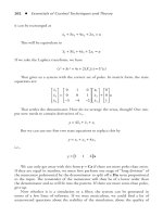
Of course, as larger squares are considered, the w-shapes will start to curve. If
we rule up the z-plane as squared graph-paper, the image in the w-plane will be
made up of “curly squares” as seen in Figure 10.1.
e illustration is a screen-grab from the code at www.esscont.com/10/z2map-
ping.htm
10.3 The Cauchy–Riemann Equations
In the previous section, we suggested that a function of z could be differentiated in
the same way that a real derivative could be found. is is true as far as “ordinary”
functions are concerned, ones that would be found in “real calculus.” However,
Figure 10.1 Illustration of mapping defined in Q 10.2.1.
91239.indb 135 10/12/09 1:43:55 PM
136 ◾ Essentials of Control Techniques and Theory
there are many more functions that can be applied to a complex variable which do
not make sense for a real one.
Consider the function w = Real(z), just the real part, x. Now w will always lie
on the real axis, and any thought of it moving in squares will make no sense. is
particular function and many more like it can possess no derivative.
If a function w(z) is to have a derivative at any given point, then for a perturba-
tion δz in z, we must be able to find a complex number (A + jB) so that around that
point δw = (A + jB)δz. Let us consider the implications of this requirement, first
looking at our example in Q 10.2.1.
w can be expressed as u + jv, so we can expand the expression to show
ujvxjy
xy jxy
+=+
=+
()
.
2
22
2−
Separating real and imaginary parts, we see the real part of w,
ux y=−
22
,
and the imaginary part
vxy= 2.
(10.2)
In general, u and v will be functions of x and y, a relationship that can be
expressed as:
uuxy= (,)
vvxy= (,)
If we make small changes δx and δy in the values of x and y, the resulting
changes in u and v will be defined by the partial derivatives in the equations:
δδδ
u
u
x
u
y
y=
∂
∂
+
∂
∂
x
and
δδδ
v
v
x
x
v
y
y=
∂
∂
+
∂
∂
.
(10.3)
91239.indb 136 10/12/09 1:43:58 PM
More Frequency Domain Background Theory ◾ 137
By holding the change in y to zero, we can clearly see that ∂u/∂x is the gradient
of u, if x is changed alone. Similarly, the three other partial derivatives are gradients
when just one variable is changed.
Now,
δδ δ
δδ δδ
wujv
u
x
x
u
y
yj
v
x
v
y
=+
=
∂
∂
+
∂
∂
+
∂
∂
+
∂
∂
x
yy
u
x
v
x
x
u
y
j
v
y
=
∂
∂
+
∂
∂
+
∂
∂
+
∂
∂
j δ
=
∂
∂
+
∂
∂
+
∂
∂
∂
∂
δ
δδ
y
u
x
j
v
x
x
v
y
j
u
y
jy−
(10.4)
If w is to have a derivative, we must be able to write
δδδ
wAjB xjy=+ +()(),
so we can equate coefficients to obtain
A
u
x
v
y
=
∂
∂
=
∂
∂
and
B
v
x
u
y
=
∂
∂
=
∂
∂
− .
(10.5)
Leave out A and B and these are the Cauchy–Riemann equations.
e main interest of such mappings from the control point of view is the “curly
squares” approximation for estimating fine detail. e Cauchy–Riemann equa-
tions partly express the condition for a function to be “analytic.” Beware, though.
Analytic behavior may be restricted to portions of the plane, and strange things
happen at a singularity such as a pole.
Q 10.3.1
Show that the Cauchy–Riemann equations hold for the functions of the example
worked out in Equations 10.2.
91239.indb 137 10/12/09 1:44:00 PM
138 ◾ Essentials of Control Techniques and Theory
10.4 Complex Integration
In real calculus, integration can be regarded as the inverse of differentiation. If
we want to evaluate the integral of f(x) from 1 to 5, we look for a function F(x) of
which f(x) is the derivative. We work out F(5) – F(1), and are satisfied to write that
down as the answer. Will the same technique work for complex integration?
In the real case, this integral is the limit of the sum of small contributions
fx x() ,
δ
where the total of the δx values takes x from 1 to 5. ere is clearly just one answer
(for a “well behaved” function). In the complex case, we can define a similar inte-
gral as the sum of contributions
fz z() .
δ
is time the answer is not so cut and dried. e trail of infinitesimal δz’s must
take us from z = 1 to z = 5, but now we are not constrained to the real axis but can
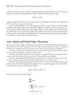
wander around the z-plane. We have to define the path, or “contour,” along which
we intend to integrate, as seen in Figure 10.2.
With luck, Cauchy’s theorem can come to our rescue. If we can find a simple
curve that encloses a region of the z-plane in which the function is everywhere
regular (analytic without singularities), then it can be shown that any path between
the endpoints lying completely within the region will give the same answer. is
B
A
z
1
z
2
δz
C
Figure 10.2 Contour integrals in the z-plane.
91239.indb 138 10/12/09 1:44:02 PM
More Frequency Domain Background Theory ◾ 139
is the same as saying that the integral around a loop in the region, starting, and
ending at the same point, will be zero.
If our path encircles a pole, it is a different matter entirely. Consider the case
where f(z) is 1/z and our path is an anticlockwise circle around the origin from
z = 1 to z = 1 again. We know that the integral of 1/z is ln(z) (the “natural” log
to base e of z) so we can write down the answer as ln(1) – ln(1). But this will not
be zero!
e logarithm is not a single-valued function when we are dealing with com-
plex variables. If we express z as re
jθ
then we see that ln(z) = ln(r) + jθ. If we take
an anticlockwise trip around the origin, the vector representing z will have rotated
through a complete circle and the value of θ will have increased by 2π. Our integral
would therefore have the value 2πj.
We could take another trip around the circle to increase θ to 4πj, and so on.
With anticlockwise or clockwise circuits, θ can take any value 2nπj, where n is an
integer positive or negative. Clearly θ will clock up a change of 2πj if z takes any
trip around the origin, the singularity, but for a journey around a small local circuit
θκ will return to the same value, as illustrated in Figure 10.3.
In the case of f(z) = 1/z, the integral in question will have the value 2πj. For
f(z) = 7/z, the integral would be 14πj. For f(z) = cos(z)/z, the integral would have
the value 2πj—since cos(0) = 1. In general, the integral around a simple pole at
z = a will be 2πj times the residue at the pole, that is the limiting value of (z – a)
f(z) as z tends to a.
e residue can be thought of as the value of the function when the offending
factor of the denominator is left out. We can turn this around the other way and
say that if f(z) is regular inside the unit circle (or any other loop for that matter),
then we can find out the value of f(a) (a is inside the loop) by integrating f(z)/(z – a)
around the loop to obtain 2πjf(a). It seems to be doing things the hard way, but it
has its uses.
z
θ
r
r
θ
z
(a) (b)
Figure 10.3 Evaluating log(z) around a contour.
91239.indb 139 10/12/09 1:44:03 PM
140 ◾ Essentials of Control Techniques and Theory
Before we leave this topic, let us establish some facts for a later chapter.
Integrating 1/z around the unit circle gives the value 2πj. Integrating 1/z
2
gives
the value zero. Its general integral is –1/z, and this is no longer multi-valued. In
fact, the integral of z
n
around the circle for any integer n will be zero, except for
n = –1.
If f(z) can be represented by a power series in 1/z,
fz az
n
n
() ,=
−
∑
then we can pick out the coefficient an by multiplying f(z) by z
n – 1
and integrat-
ing around the unit circle. is gives us a transform between sequences of values
an and a function of z. We can construct the function of z simply by multiplying
the coefficients by the appropriate powers of z and summing (all right, there is the
question of convergence), and we can unravel the coefficients again by the integral
method.
is transform between a sequence of values and a function of z will become
important when we consider sampled data systems in more detail. But first there
are two more transforms that are relevant to continuous systems, the Laplace trans-
form and the Fourier transform.
10.5 Differential Equations and the Laplace Transform
In Chapter 2 we glanced at the problems of finding analytic solutions to differential
equations. Now we will look at an alternative approach that will give a rigorous
solution.
Suppose we have a function of time, f(t), and that we are really only interested
in its values for t > 0. For reasons we will see later, we can multiply f(t) by the
exponential function e
–st
and integrate from t = 0 to infinity. We can write the
result as
Fs ftedt
st
() () .=
∞
∫
−
0
e result is written as F(s), because since the integral has been evaluated over a
defined range of t, t has vanished from the resulting expression. On the other hand,
the result will depend on the value chosen for s. In the same way that we have been
thinking of f(t) not as just one value but as a graph of f(t) plotted against time,
so we can consider F(s) as a function defined over the entire range of s. We have
transformed the function of time, f(t), into a function of the variable s. is is the
“unilateral” Laplace transform.
Consider an example. e Laplace transform of the function 5e
–at
is given by
91239.indb 140 10/12/09 1:44:04 PM
More Frequency Domain Background Theory ◾ 141
0
0
5
5
5
∞
∞
+
+
∫
∫
=
=
+
edt
edt
sa
e
at st
sat
sat
−−
−
−
−
e
()
()
[[]
=
+
∞
0
5
sa
.
We have a transform that turns functions of t into functions of s. Can we work
the trick in reverse? Given a function of s, can we find just one function of time of
which it is the transform? We may or may not arrive at a precise mathematical pro-
cess for finding the “inverse”—it is sufficient to spot a suitable function, provided
that we can show that the answer is unique.
For “well-behaved” functions, we can show that the transform of the sum of
two functions is the sum of the two transforms:
L {()()} {()()}
{()}
ft gt ft gt edt
ft
st
+= +
=
∞
∞
∫
∫
−
0
0
eedtgte dt
Fs Gs
st st−−
+
=+
∞
∫
0
{()}
() ().
Now suppose that two functions of time, f(t) and g(t), have the same Laplace
transform. en the Laplace transform of their difference must be zero:
L{()()} () ()ft gt Fs Gs−−==0
since we have assumed F(s) = G(s). What values can [f(t) – g(t)] take, if its Laplace
integral is zero for every value of s? It can be shown that if we require f(t) – g(t) to be
differentiable, then it must be zero for all t > 0; in other words the inverse transform
(if it exists) is unique.
Why should we be interested in leaving the safety of the time domain for these
strange functions of s? Consider the transform of the derivative of f(t):
L{()} () .
′
=
′
∞
∫
ft ftedt
st
0
−
91239.indb 141 10/12/09 1:44:06 PM
142 ◾ Essentials of Control Techniques and Theory
Integrating by parts, we see
L{()} [()] () ()
′
=−
=
∞
∞
∫
ft fteft
d
dt
edt
f
-stst
0
0
−
− (() () ()
() ().
0
0
0
−−
−
−
sfte dt
sF sf
st
∞
∫
=
We can use this result to show that
LL{()} {()} ()
() () (
′′
=
′′
=
′′
ft sftf
sFssff
−
−−
0
0
2
00)
and in general
L{()} () () ()
() ()
ft sFssfsff
nnnn n
=− −
−− −12 1
00
′
… (().0
So what is the relevance of all this to the solution of differential equations?
Suppose we are faced with
xx e
at
+=
−
5
(10.6)
Now, if
L{()}xt
is written as X(s), we have
L{} () () ()
xsXs sx x=
2
00−−
so we can express the transform of the left-hand side as
L{}()() () ().
xx sXssxx++−−=
2
100
For the right-hand side, we have already worked out that
L{} ,5
5
e
sa
at−
=
+
so
()() () () ,sXssxx
sa
2
100
5
+−−=
+
91239.indb 142 10/12/09 1:44:10 PM
More Frequency Domain Background Theory ◾ 143
or
Xs
ssa
sx x() () ().=
++
++
1
1
5
00
2
(10.7)
Without too much trouble we have obtained the Laplace transform of the solu-
tion, complete with initial conditions. But how do we unravel this to give a time
function? Must we perform some infinite contour integration or other? Not a bit!
e art of the Laplace transform is to divide the solution into recognizable
fragments. ey are recognizable because we can match them against a table of
transforms representing solutions to “classic” differential equations. Some of the
transforms might have been obtained by infinite integration, as we showed with
e
–at
, but others follow more easily by looking at differential equations.
e general solution to
xx+=0
is
xA tB t=+cos( )sin().
Now
L{}
xx+=0
so
Xs
s
sx x() [()()].=
+
+
1
1
00
2
For the function x = cos(t), x(0) = 1, and
x
()00=
, then
L{cos()}.t
s
s
=
+
2
1
If x = sin(t), x(0) = 0, and
x()01=
, then
L{sin()}.t
s
=
+
1
1
2
With these functions in our table, we can settle two of the terms of Equation 10.7.
We are left, however, with the term:
1
1
5
2
ssa++
91239.indb 143 10/12/09 1:44:14 PM
144 ◾ Essentials of Control Techniques and Theory
Using partial fractions, we can crack it apart into
ABs
s
C
sa
+
+
+
+
2
1
.
Before we know it, we find ourselves having to solve simultaneous equations to
work out A, B, and C. ese are equivalent to the equations we would have to solve
for the initial conditions in the straightforward “particular integral and comple-
mentary function” method.
Q 10.5.1
Find the time solution of differential equation 10.6 by solving for A, B, and C in
transform 10.7 and substituting back from the known transforms. en solve the
original differential equation the “classic” way and compare the algebra involved.
e Laplace transform really is not a magical method of solving differential
equations. It is a systematic method of reducing the equations, complete with initial
conditions, to a standard form. is allows the solution to be pieced together from a
table of previously recognized functions. Do not expect it to perform miracles, but
do not underestimate its value.
10.6 The Fourier Transform
After battling with Laplace, the Fourier transform may seem rather tame. e
Laplace transformation involved the multiplication of a function of time by e
–st
and
its integration over all positive time. e Fourier transform requires the time func-
tion to be multiplied by e
–jωt
and then integrated over all time, past, and future.
It can be regarded as the analysis of the time function into all its frequency
components, which are then presented as a frequency spectrum. is spectrum also
contains phase information, so that by adding all the sinusoidal contributions the
original function of time can be reconstructed.
Start by considering the Fourier series. is can represent a repetitive function
as the sum of sine and cosine waves. If we have a waveform that repeats after time
2T, it can be broken down into the sum of sinusoids of period 2T, together with
their harmonics.
Let us set out by constructing a repetitive function of time in this way. Rather
than fight it out with sines and cosines, we can allow the function to be complex,
and we can take the sum of complex exponentials:
ft ce
n
n
T
jt
n
() .=
=−∞
∞
∑
π
(10.8)
91239.indb 144 10/12/09 1:44:15 PM
More Frequency Domain Background Theory ◾ 145
Can we break f(t) back down into its components? Can we evaluate the coef-
ficients cn from the time function itself?
e first thing to notice is that because of its cyclic nature, the integral of e
nπjt/T
from t = –T to +T will be zero for any integer n except zero. If n = 0, the exponential
degenerates into a constant value of unity and the value of the integral will be just
2T.
Now if we multiply f(t) by e
–rπt/T
, we will have the sum of terms:
fte
rtTnrtT
n
() .
/()/−−
=−∞
∞
=
∑
π
ce
n
π
If we integrate over the range t = –T to +T, the contribution of every term on the
right will vanish, except one. is will be the term where n = r, and its contribution
will be 2Tc
r
.
We have a route from the coefficients to the time function and a return trip
back to the coefficients.
We considered the Fourier series as a representation of a function which repeated
over a period 2T, i.e., where its behavior over t = –T to +T was repeated again and
again outside those limits. If we have a function that is not really repetitive, we can
still match its behavior in the range t = –T to +T with a Fourier series (Figure 10.4).
e lowest frequency in the series will be π/T. e series function will match
f(t) over the center range, but will be different outside it. If we want to extend
the range of the matching section, all we have to do is to increase the value of T.
Suppose that we double it, then we will halve the lowest frequency present, and
the interval between the frequency contributions will also be halved. In effect, the
number of contributing frequencies in any range will be doubled.
We can double T again and again, and increase the range of the match indefi-
nitely. As we do so, the frequencies will bunch closer and closer until the summa-
tion of Equation 10.8 would be better written as an integral. But an integral with
respect to what?
f(t)
Fourier
approximation
–T
T
Figure 10.4 A Fourier series represents a repetitive waveform.
91239.indb 145 10/12/09 1:44:16 PM