Essentials of Control Techniques and Theory_10 pptx

More about Time and State Equations ◾ 229
But now the concept of rank gets more interesting. What is the rank of

1002
0103
0014










e first three columns are clearly independent, but the fourth cannot add to
the rank. e rank is three. So what has this to do with controllability?
Suppose that our system is of third order. en by manipulating the inputs, we
must be able to make the state vary through all three dimensions of its variables.


xAxBu=+
If the system has a single input, then the B matrix has a single column. When
we first start to apply an input we will set the state changing in the direction of that
single column vector of B. If there are two inputs then B has two columns. If they
are independent the state can be sent in the direction of any combination of those
vectors. We can stack the columns of B side by side and examine their rank.
But what happens next? When the state has been sent off in such a direction, the
A matrix will come into play to move the state on further. e velocity can now be
in a direction of any of the columns of AB. But there is more. e A matrix can send

each of these new displacements in the direction A
2
B, then A
3
B and so on forever.
So to test for controllability we look at the rank of the composite matrix

BABABAB
23

[]
It can be shown that in the third order case, only the first three terms need be
considered. e “Cayley Hamilton” theory shows that if the second power of A has
not succeeded in turning the state to cover any missing directions, then no higher
powers can do any better.
In general the rank must be equal to the order of the system and we must
consider terms up to
AB
n−1
.
It is time for an example.
Q 16.6.1
Is the following system controllable?


xx=
−−







+






01
12
0
1
u
91239.indb 229 10/12/09 1:46:28 PM
230 ◾ Essentials of Control Techniques and Theory
Now

AB =
−−













=
−






01
12
0
1
1
2
so

BAB
[]
=
−






01

12
which has rank 2. e system is controllable.
Q 16.6.2
Is this system also controllable?


xx=
−−






+
−






01
12
1
1
u
Q 16.6.3
Is this third system controllable?


xx=
−−






+






01
12
1
0
u
Q 16.6.4
Express that third system in Jordan Canonical Form. What is the simulation
structure of that system?
Can we deduce observability in a similar simple way, by looking at the rank of
a set of matrices?
e equation

yCx=
is likely to represent fewer outputs than states; we have not enough simultaneous

equations to solve for x. If we ignore all problems of noise and continuity, we can
consider differentiating the outputs to obtain
91239.indb 230 10/12/09 1:46:30 PM
More about Time and State Equations ◾ 231


yCx
C(Ax Bu)
=
=+
so


yCBu−
can provide some more equations for solving for x. Further differentiation will give
more equations, and whether these are enough can be seen by examining the rows
of C, of CA and so on, or more formally by testing the rank of

C
CA
CA
CA
2
1

n−

















and ensuring that it is the same as the rank of the system.
Showing that the output can reveal the state is just the start. We now have to
find ways to perform the calculation without resorting to differentiation.
91239.indb 231 10/12/09 1:46:32 PM
This page intentionally left blank
233
17Chapter
Practical Observers,
Feedback with Dynamics
17.1 Introduction
In the last chapter, we investigated whether the inputs and outputs of a system
made it possible to control all the state variables and deduce their values. ough
the tests looked at the possibility of observing the states, they did not give very
much guidance on how to go about it.
It is unwise, to say the least, to try to differentiate a signal. Some devices that
claim to be differentiators are in fact mere high-pass filters. A true differentiator
would have to have a gain that tends to infinity with increasing frequency. Any
noise in the signal would cause immense problems.

Let us forget about these problems of differentiation, and instead address the
direct problem of deducing the state of a system from its outputs.
17.2 The Kalman Filter
First we have to assume that we have a complete knowledge of the state equations.
Can we not then set up a simulation of the system, and by applying the same inputs
simply measure the states of the model? is might succeed if the system has only
poles that represent rapid settling—the sort of system that does not really need
feedback control!
91239.indb 233 10/12/09 1:46:33 PM
234 ◾ Essentials of Control Techniques and Theory
Suppose instead that the system is a motor-driven position controller. e
output involves integrals of the input signal. Any error in setting up the initial
conditions of the model will persist indefinitely.
Let us not give up the idea of a model. Suppose that we have a measurement of
the system’s position, but not of the velocity that we need for damping. e position
is enough to satisfy the condition for observability, but we do not wish to differenti-
ate it. Can we not use this signal to “pull the model into line” with the state of the
system? is is the principle underlying the “Kalman Filter.”
e system, as usual, is given by


xAxBu
yCx
=+
=
(17.1)
We can set up a simulation of the system, having similar equations, but where
the variables are
ˆ
x

and
ˆ
y
. e “hats” mark the variables as estimates. Since we know
the value of the input, u, we can use this in the model.
Now in the real system, we can only influence the variables through the input
via the matrix B. In the model, we can “cheat” and apply an input signal directly to
any integrator and hence to any state variable that we choose. We can, for instance,
calculate the error between the measured outputs, y, and the estimated outputs
ˆ
y

given by
Cx
ˆ
, and mix this signal among the state integrators in any way we wish.
e model equations then become

ˆˆ
(
ˆ
)
ˆˆ

xAxBuKyCx
yCx
=++−
=
(17.2)
e corresponding system is illustrated in Figure 17.1.

e model states now have two sets of inputs, one corresponding to the plant’s
input and the other taken from the system’s measured output. e model’s A-matrix
has also been changed, as we can see by rewriting 17.2 to obtain

ˆ
()
ˆ

xAKC xBuKy=− ++
(17.3)
To see just how well we might succeed in tracking the system state variables, we
can combine Equations 17.1 through 17.3 to give a set of differential equations for
the estimation error,
xx−
ˆ
:

d
dt
(
ˆ
)( )(
ˆ
)xx AKCx x−= −−
(17.4)
91239.indb 234 10/12/09 1:46:36 PM
Practical Observers, Feedback with Dynamics ◾ 235
e eigenvalues of (A – KC) will determine how rapidly the model states settle
down to mimic the states of the plant. ese are the roots of the model, as defined
in Equation 17.3. If the system is observable, we should be able to choose the coef-

ficients of K to place the roots wherever we wish; the choice will be influenced by
the noise levels we expect to find on the signals.
Q 17.2.1
A motor is described by two integrations, from input drive to output position. e
velocity is not directly measured. We wish to achieve a well-damped position con-
trol, and so need a velocity term to add. Design a Kalman observer.
e system equations for this example may be written


xx
yx
=
=
01
00
0
1
10






+







[]
u
(17.5)
e Kalman feedback matrix will be a vector (p, q)′ so the structure of the filter
will be as shown in Figure 17.2.
B
+
C
A
B
+
C
A
K
+
–
u
x
y
x
^
x
^
All estimated states
available for feedback
Model
Figure 17.1 Structure of Kalman Filter.
91239.indb 235 10/12/09 1:46:38 PM
236 ◾ Essentials of Control Techniques and Theory

For the model, we have

AKC
p
q
p
q
−=






−






[]
=
−
−







01
00
10
1
0
e eigenvalues are given by the determinant det(A–KC–λI), i.e.,

λλ
2
0++=pq.
We can choose the parameters of K to put the roots wherever we like.
It looks as though we now have both position and velocity signals to feed around
our motor system. If this is really the case, then we can put the closed loop poles
wherever we wish. It seems that anything is possible—keep hoping.
+
–
q
p
Motor
u
y
.
^
y
^
y
Figure 17.2 Kalman filter to observe motor velocity.
91239.indb 236 10/12/09 1:46:40 PM
Practical Observers, Feedback with Dynamics ◾ 237

Q 17.2.2
Design observer and feedback for the motor of Equation 17.5 to give a response
characteristic having two equal roots of 0.1 seconds, with an observer error charac-
teristic having equal roots of 0.5 seconds. Sketch the corresponding feedback circuit
containing integrators.
17.3 Reduced-State Observers
In the last example, it appeared that we have to use a second-order observer to
deduce a single state variable. Is there a more economic way to make an observer?
Luenberger suggested the answer.
Suppose that we do not wish to estimate all the components of the state, but
only a selection given by Sx. We would like to set up a modeling system having
states z, while it takes inputs u and y. e values of the z components must tend to
the signals we wish to observe. is appears less complicated when written algebra-
ically! e observer equations are


zPzQuRy=+ +
(17.6 )
and we want all the components of (z–Sx) to tend to zero in some satisfactory way.
Now we see that the derivative of (z–Sx) is given by



zSxPzQuRyS(AxBu)
Pz Qu RCxSAx SBu
−=++−+
=+ +−−
= PPz (RCSA)x(QSB)u+− +−
We would like this to reduce to



zSxP(z Sx)−= −
where P represents a system matrix giving rapid settling. For this to be the case,

−= −PS (RCSA)
and

QSB0−=
91239.indb 237 10/12/09 1:46:42 PM
238 ◾ Essentials of Control Techniques and Theory
i.e., when we have decided on S that determines the variables to observe, we have

QSB,=
(17.7)

RC SA PS=−.
(17.8)
Q 17.3.1
Design a first-order observer for the velocity in the motor problem of Equation 17.5.
Q 17.3.2
Apply the observed velocity to achieve closed loop control as specified in problem
Q 17.2.2.
e first problem hits an unexpected snag, as you will see.
If we refer back to the system state equations of 17.5, we see that


xx
yx
=







+






=
[]
01
00
0
1
10
u
If we are only interested in estimating the velocity, then we have

S = [,].01
Now

QSB==
[]







=01
0
1
1
P becomes a single parameter defining the speed with which z settles, and we may
set it to a value of –k.

SA PS−=
[]






−−
[][]
=
[]
+
[]
01
01
00
01
000

k
k
91239.indb 238 10/12/09 1:46:44 PM
Practical Observers, Feedback with Dynamics ◾ 239
We now need R, which in this case will be a simple constant r, such that

RC SA PS=−
i.e.,

rk[1,0] [0,]=
and there is the problem! Clearly there is no possible combination to make the
equation balance except if r and k are both zero.
Do not give up! We actually need the velocity so that we can add it to a position
term for feedback. So suppose that instead of pure velocity, we try for a mixture of
position plus a times the velocity. en

Sx x= [1,]a .
For Q we have the equation

QSB==
[]






=1
0
1

aa
is time

SA PS−=
[]






−−
[][]
=
[]
+
[]
=
1
01
00
1
01
1
aka
kka
k ++
[]
ka
Now we can equate this to RC if

rk=
and

(1+=ka)0.
From this last equation we see that a must be negative, with value –1/k. at
would be the wrong sign if we wished to use this mixture alone as feedback.
91239.indb 239 10/12/09 1:46:47 PM
240 ◾ Essentials of Control Techniques and Theory
However, we can subtract z from the position signal to get a mixture that has the
right sign.

zxax
xkx
=+
=−


ˆ
(/ )
ˆ
1
so the estimated velocity will be given by


ˆ
()xkxz=−
where



zzuy
kz ku kx
=++
=− −+
PQR
(/ )1
Mission accomplished.
To see it in action, let us attack problem Q 17.3.2. We require a response similar
to that specified in Q 17.2.2. We want the closed loop response to have equal roots
of 0.1 seconds, now with a single observer settling time constant of 0.5 seconds.
For the 0.5 second observer time constant, we make k = 2.
For the feedback we now have all the states (or their estimates) available, so
instead of considering (A + BFC) we only have (A + BF) to worry about. To achieve
the required closed loop response we can propose algebraic values for the feedback
parameters in F, substitute them to obtain (A + BF) and then from the eigen-
value determinant derive the characteristic equation. Finally we equate coefficients
between the characteristic equation and the equation with the roots we are trying
to fiddle. Sounds complicated?
In this simple example we can look at its system equations in the “traditional
form”


xu= .
e two time constants of 0.1 seconds imply root values of 10, so when the loop
is closed the behavior of x must be described by

 
xx x++ =20 100 0
so

uxx=− −100 20

91239.indb 240 10/12/09 1:46:50 PM
Practical Observers, Feedback with Dynamics ◾ 241
Instead of he velocity we must use the estimated velocity, so we must set the system
input to

uxx=− −100 20

ˆ

ux xz=− −× −100 20 2( )

uxz=− +140 40
where z is given by the subsystem we have added


zzuy=− −+2052.
where the output signal y is the position x.
Before leaving the problem, let us look at the observer in transfer function
terms. We can write

() .sZ UY+=−+2052
so the equation for the input u becomes

UYZ=− +140 40

=− +
−+
+

140 40
05 2
2
Y
UY
s
.
So, tidying up and multiplying by (s + 2) we have

() ()
()(
sU UsYY
sU s
++ =− ++
+=−+
220 140 280
22 140 200))Y
U
s
s
Y=−
+
+
140 200
22
e whole process whereby we calculate the feedback input u from the position
output y has boiled down to nothing more than a simple phase advance! To make
matters worse, it is not even a very practical phase advance, since it requires the
91239.indb 241 10/12/09 1:46:54 PM
242 ◾ Essentials of Control Techniques and Theory

high-frequency gain to be over 14 times the gain at low frequency. We can certainly
expect noise problems from it.
Do not take this as an attempt to belittle the observer method. Over the years,
engineers have developed intuitive techniques to deal with common problems, and
only those techniques which were successful have survived. e fact that phase
advance can be shown to be equivalent to the application of an observer detracts
from neither method—just the reverse.
By tackling a problem systematically, analyzing general linear feedback of states
and estimated states, the whole spectrum of solutions can be surveyed to make a
choice. e reason that the solution to the last problem was impractical had noth-
ing to do with the method, but depended entirely on our arbitrary choice of settling
times for the observer and for the closed loop system. We should instead have left
the observer time constant as a parameter for later choice, and we could then have
imposed some final limitation on the ratio of gains of the resulting phase advance.
rough this method we would at least know the implications of each choice.
If the analytic method does have a drawback, it is that it is too powerful. e
engineer is presented with a wealth of possible solutions, and is left agonizing over
the new problem of how to limit his choice to a single answer. Some design meth-
ods are tailored to reduce these choices. As often as not, they throw the baby out
with the bathwater.
Let us go on to examine linear control in its most general terms.
17.4 Control with Added Dynamics
We can scatter dynamic filters all around the control system, as shown in
Figure 17.3.
e signals shown in Figure 17.3 can be vectors with many components. e
blocks represent transfer function matrices, not just simple transfer functions. is
means that we have to use caution when applying the methods of block diagram
manipulation.
In the case of scalar transfer functions, we can unravel complicated structures
by the relationships illustrated in Figure 17.4.

V
F(s)
K(s)
G(s)
H(s)
Y
+
Figure 17.3 Feedback around G(s) with three added filters.
91239.indb 242 10/12/09 1:46:55 PM
Practical Observers, Feedback with Dynamics ◾ 243
Now, however complicated our controller may be, it simply takes inputs
from the command input v and the system output y and delivers a signal to the
system input u. It can be described by just two transfer function matrices. We
have one transfer function matrix that links the command input to the system
input, which we will call the feedforward matrix. We have another matrix link-
ing the output back to the system input, not surprisingly called the feedback
matrix.
If the controller has internal state z, then we can append these components
to the system state x and write down a set of state equations for our new, bigger
system.
Suppose that we started with


xAxBu
yCx
=+
=
A(s)
B(s)
=

A(s)
B(s)
A(s)
B(s)
A(s)+B(s)
+
A(s) B(s)
A(s)B(s)
A(s)
1–A(s)B(s)
C(s)
+
=
=
=
A(s)C(s)
B(s)
C(s)
(b)
(a)
(c)
(d)
Figure 17.4 Some rules of block diagram manipulation.
91239.indb 243 10/12/09 1:46:57 PM
244 ◾ Essentials of Control Techniques and Theory
and added a controller with state z, where


zKzLyMv=++
We apply signals from the controller dynamics, the command input and the

system output to the system input, u,

uFyGzHv=++
so that


x(ABFC)x BGzBHv=+ ++
and


zLCx Kz Mv=++
We end up with a composite matrix state equation



x
z
ABFC BG
LC K
x
z
BH
M






=

+












+






v
We could even consider a new “super output” by mixing y, z, and v together,
but with the coefficients of all the matrices F, G, H, K, L, and M to choose, life is
difficult enough as it is.
Moving back to the transfer function form of the controller, is it possible or
even sensible to try feedforward control alone? Indeed it is.
Suppose that the system is a simple lag, slow to respond to a change of demand.
It makes sense to apply a large initial change of input, to get the output moving,
and then to turn the input back to some steady value.
Suppose that we have a simple lag with time constant five seconds, described by

transfer function

1
15+ s
If we apply a feedforward filter at the input, having transfer function

15
1
+
+
s
s
91239.indb 244 10/12/09 1:46:59 PM
Practical Observers, Feedback with Dynamics ◾ 245
(here is that phase advance again!), then the overall response will have the form:

1
1+ s
e five-second time constant has been reduced to one second. We have can-
celed a pole of the system by putting an equal zero in the controller, a technique
called pole cancellation. Figure 17.5 shows the effect.
Take care. Although the pole has been removed from the response, it is still
present in the system. An initial transient will decay with a five-second time con-
stant, not the one second of our new transfer function. Moreover, that pole has
been made uncontrollable in the new arrangement.
Step response of
1
1+5s
1
1+5s

Step response of
y(t)
u(t)
v(t)
u(t)
y(t)
1+5s
1+s
v(t)
u(t)
y(t)
Figure 17.5 Responses with feedforward pole cancellation.
91239.indb 245 10/12/09 1:47:01 PM
246 ◾ Essentials of Control Techniques and Theory
If it is benign, representing a transient that dies away in good time, then we can
bid it farewell. If it is close to instability, however, then any error in the controller
parameters or any unaccounted “sneak” input or disturbance can lead to disaster.
If we put on our observer-tinted spectacles, we can even represent pole-
canceling feedforward in terms of observed state variables. e observer in this
case is rather strange in that z can receive no input from y, otherwise the controller
would include feedback. Try the example:
Q 17.4.1
Set up the state equations for a five-second lag. Add an estimator to estimate the
state from the input alone. Feed back the estimated state to obtain a response with
a one-second time constant.
17.5 Conclusion
Despite all the sweeping generalities, the subject of applying control to a system is
far from closed. All these discussions have assumed that both system and controller
will be linear, when we saw from the start that considerations of signal and drive
limiting can be essential.

91239.indb 246 10/12/09 1:47:01 PM
247
18Chapter
Digital Control in
More Detail
18.1 Introduction
e philosophers of Ancient Greece found the concept of continuous time quite
baffling, getting tied up in paradoxes such as that of Xeno. Today’s students are
brought up on a diet of integral and differential calculus, taking velocities and
accelerations in their stride, so that it is finite differences which may appear quite
alien to them.
But when a few fundamental definitions have been established, it appears clear
that discrete time systems can be managed more expediently than continuous ones.
It is when the two are mixed that the control engineer must be wary.
Even so, we will creep up on the discrete time theory from a basis of continuous
time and differential equations.
18.2 Finite Differences—The Beta-Operator
We built our concepts of continuous control on the differential operator, “rate-of-
change.” We let time change by a small amount δt, resulting in a change of x(t)
given by

δδ
xxttxt=+−()()
then we examined the limit of the ratio δx/δt as we made δt tend to zero.
91239.indb 247 10/12/09 1:47:03 PM
248 ◾ Essentials of Control Techniques and Theory
Now we have let a computer get in on the act, and the rules must change.
x(t) is measured not continuously, but at some sequence of times with fixed
intervals. We might know x(0), x(0.01), x(0.02), and so on, but between these val-
ues the function is a mystery. e idea of letting δt tend to zero is useless. e only

sensible value for δt is equal to the sampling interval. It makes little sense to go on
labeling the functions with their time value, x(t). We might as well acknowledge
them to be a sequence of discrete samples, and label them x(n) according to their
sample number.
We must be satisfied with an approximate sort of derivative, where δt takes a
fixed value of one sampling interval, τ. We are left with another subtle problem
which is important nonetheless. Should we take our difference as “next value minus
this one,” or as “this value minus last one?” If we could attribute the difference to
lie at a time midway between the samples there would be no such question, but
that does not help when we have to tag variables with “sample number” rather than
time.
e point of the system equations, continuous or discrete time, is to be able
to predict the future state from the present state and the input. If we have the
equivalent of an integrator that is integrating an input function g(n), we might
write

fn fn gn()() (),+= +1
τ
(18.1)
which settles the question in favor of the forward difference

gn fn fn() {( )()}/.=+−1
τ
It looks as though we can only calculate g(n) from the f(n) sequence if we already
know a future value, f(n + 1). In the continuous case, however, we always dealt with
integrators and would not consider differentiating a signal, so perhaps this will not
prove a disadvantage.
We might define this approximation to differentiation as an operator, β, where
inside it is a “time advance” operation that looks ahead:

β
τ
(())
()()
fn
fn fn
=
+−1
(18.2)
We could now write

gn fn() (()),=
β
91239.indb 248 10/12/09 1:47:05 PM
Digital Control in More Detail ◾ 249
where we might in the continuous case have used a differential operator to write

gt
d
dt
ft() ().=
e inverse of the differentiator is the integrator, at the heart of all continuous
simulation.
e inverse of the β-operator is the crude numerical process of Euler integration
as in Equation 18.1.
Now the second order differential equation

 
xaxbxu++=
might be approximated in discrete time by

ββ
2
xaxbxu++=
Will we look for stability in the same way as before? You will remember that we
looked at the roots of the quadratic

mamb
2
0++=
and were concerned that all the roots should have negative real parts. is concern
was originally derived from the fact that e
mt
was an “eigenfunction” of a linear
differential equation, that if an input e
mt
was applied, the output would be pro-
portional to the same function. Is this same property true of the finite difference
operator β?
We can calculate

β
τ
τ
ττ
()
()
e
ee
m

mm
=
−
+1

=
−e
e
m
τ
τ
τ
1
is is certainly proportional to e
mτ
. We would therefore be wise to look for the
roots of the characteristic equation, just as before, and plot them in the complex
plane.
91239.indb 249 10/12/09 1:47:07 PM
250 ◾ Essentials of Control Techniques and Theory
Just a minute, though. Will the imaginary axis still be the boundary between
stable and unstable systems? In the continuous case, we found that that a sinewave,
e
jωt
, emerged from differentiation with an extra multiplying factor jω, represented
by a point on the imaginary axis. Now if we subject the sinewave to the β-operator
we get

β
−

τ
ω
ωτ
ω
()e
e
e
jt
j
jt
=
1
As ω varies, the gain moves along the locus defined by

g
r
==real part
cos( )
,
ωτ
τ
−1

g
i
==imaginarypart
sin( )
.
ωτ
τ

So

() .
ττ
gg
ri
++ =11
22
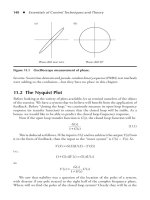
is is a circle, center –1/τ, radius 1/τ, which touches the imaginary axis
at the origin but curves round again to cut the real axis at –2/τ. It is shown in
Figure 18.1.
It is not hard to show that for stability the roots of the characteristic equation
must lie inside this circle.
–2
–1
τ
τ
Figure 18.1 β-plane stability circle.
91239.indb 250 10/12/09 1:47:10 PM
Digital Control in More Detail ◾ 251
e system


xax=−
has a pole at –a, and is stable no matter how large a is made. On the other hand,
the discrete time approximation to this system

βxax=−
also has a pole at –a, but if a is increased to beyond 2/τ the pole emerges from the
left margin of the stability circle, and oscillation results. is is the step length

problem in another guise.
If we take a set of poles in the s-plane and approximate them by poles in the
same position in the β-plane, they must be considerably nearer to the origin than
1/τ for the approximation to ring true. If we want a near-perfect representation, we
must map the s-poles to β-poles in somewhat different locations. en again, the
β-plane might not give the clearest impression of what is happening.
18.3 Meet the z-Transform
In Chapter 8, we took a quick glance at the z-operator. We needed to use the com-
puter to deduce a velocity signal for controlling the inverted pendulum. Now it is
time to consider discrete time theory in more rigorous detail.
e β-operator is a discrete time approximation to differentiation, the coun-
terpart of Euler integration. In Section 2.6 we were able to solve the differential
equations to derive an exact simulation that is accurate for any step length. at
corresponds to the z-transform.
We saw the Laplace transform defined in terms of an infinite integral

L xt xtedt
st
() () .
(
)
=
−
∞
∫
0
(18.3)
Now, instead of continuous functions of time, we must deal with sequences of
discrete numbers x(n), each relating to a sampled value at time nτ.
We define the z-transform as

Z xn xnz
n
n
() () .
(
)
=
−
=
∞
∑
0
(18.4)
91239.indb 251 10/12/09 1:47:12 PM
252 ◾ Essentials of Control Techniques and Theory
Even though we know that we can extract x(r) by multiplying the transform by z
r

and integrating around a contour that circles z = 0, why on earth would we want to
complicate the sequence in this way?
e answer is that most of the response functions we meet will be exponentials
of one sort or another. If we consider a sampled version of e
–at
we have

xn e
an
()=
−

τ
so the z-transform is

ez
an n
n
−τ−
=
∞
∑
0

=
=
−
=
−
−−
=
∞
−−
−
∑
()ez
ez
z
ze
an
n
a

a
τ
τ
τ
1
0
1
1
1
So we have in fact found our way from an infinite series of numbers to a simple
algebraic expression, the ratio of a pole and a zero.
In exactly the same way that a table can be built relating Laplace transforms to
the corresponding time responses, a table of sequences can be built for z-transforms.
However that is not exactly what we are trying to achieve. We are more likely to use
the z-transform to analyze the stability of a discrete time control system, in terms
of its roots, rather than to seek a specific response sequence.
A table is still relevant. We are likely to have a system defined by a continuous
transfer function, which we must knit together with the z-transform representation
of a discrete time controller. But as we will see, the tables equating z and Laplace
transforms that are usually published are not the most straightforward way to deal
with the problem.
18.4 Trains of Impulses
e z-transform can be related to the Laplace transform, where an impulse modu-
lator has been inserted to sample the signal at regular intervals. ese samples
91239.indb 252 10/12/09 1:47:13 PM
Digital Control in More Detail ◾ 253
will take the form of a train of impulses, multiplied by the elements of our
number series

xn tn()()δτ−

∞
∑
0
we see that its Laplace transform is

xn tn edt
st
()()δτ−






∞
∞
−
∑
∫
0
0

xn tnedt
st
() ().
0
0
∞
∞
−

∑
∫
−δτ

xne
ns
()
0
∞
−
∑
τ
If we write z in place of e
st
this is the same expression as the z-transform.
But to associate z-transforms with inverse Laplace transforms has some serious
problems. Consider the case of a simple integrator, 1/s.
e inverse of the Laplace transform seems easy enough. We know that the
resulting time function is zero for all negative t and 1 for all positive t, but what
happens at t = 0? Should the sampled sequence be
1, 1, 1, 1, 1,
or
0, 1, 1, 1, 1, ?
Do we sample the waveform “just before” the impulse changes it or just after-
wards? Later we will see how to avoid the dilemma caused by impulses and impulse
modulators.
Q 18.4.1
What is the z-transform of the impulse-response of the continuous system whose
transfer function is 1/(s
2 

+ 3s + 2)? (First solve for the time response.) Is it the prod-
uct of the z-transforms corresponding to 1/(s + 1) and 1/(s + 2)?
91239.indb 253 10/12/09 1:47:15 PM