New Frontiers in Banking Services Emerging Needs and Tailored Products for Untapped Markets_7 doc

7.1 Hong Kong 173
1986 1988 1990 1992 1994 1996 1998 2000 2002
−0.1
0
0.1
0.2
0.3
0.4
0.5
0.6
0.7
0.8
0.9
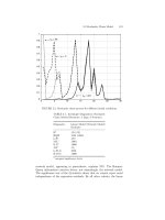
FIGURE 7.6. Price gap: Hong Kong and mainland China
and residential property price indices, as well as the price gap. However,
the price gap volatility is due in large part to the once-over Renminbi
devaluation in 1994.
Table 7.1 also shows that highest correlations of inflation are with rates of
growth of unit labor costs and property prices, followed closely by the out-
put gap. Finally, Table 7.1 shows a strong correlation between the growth
rates of the share price and the residential property price indices.
In many studies relating to monetary policy and overall economic activ-
ity, bank lending appears as an important credit channel for assessing
inflationary or deflationary impulses. Gerlach and Peng (2003) examined
the interaction between banking credit and property prices in Hong Kong.
They found that property prices are weakly exogenous and determine bank
lending, while bank lending does not appear to influence property prices
[Gerlach and Peng (2003), p. 11]. They argued that changes in bank lending
cannot be regarded as the source of the boom and bust cycle in Hong Kong.
They hypothesized that “changing beliefs about future economic prospects
led to shifts in the demand for property and investments.” With a higher

inelastic supply schedule, this caused price swings, and with rising demand
174 7. Inflation and Deflation: Hong Kong and Japan
TABLE 7.1. Statistical Summary of Data
Hong Kong Quarterly Data, 1985–2002
Property
Price Output Imp Price Price HSI ULC
Inflation Gap Gap Growth Growth Growth Growth
Mean 0.055 0.511 0.004 0.023 0.088 0.127 0.102
Std. Dev. 0.049 0.258 0.024 0.051 0.215 0.272 0.062
Correlation Matrix
Property
Price Output Imp Price Price HSI ULC
Inflation Gap Gap Growth Growth Growth Growth
Inflation 1.00
Price Gap −0.39 1.00
Output Gap 0.56 −0.29 1.00
Imp Price Growth 0.15 −0.37 0.05 1.00
Property Price Growth 0.57 −0.42 0.36 0.23 1.00
HSI Growth 0.06 −0.04 −0.15 0.43 0.56 1.00
ULC Growth 0.59 −0.84 0.48 0.29 0.38 −0.09 1.00
for loans, “bank lending naturally responded” [Gerlach and Peng (2003),
p. 11]. For this reason, we leave out the growth rate of bank lending as a
possible determinant of inflation or deflation in Hong Kong.
1,2
7.1.2 Model Specification
We draw upon the standard Phillips curve framework used by Stock and
Watson (1999) for forecasting inflation in the United States. They define
the inflation as an h-period ahead forecast. For our quarterly data set, we
set h = 4 for an annual inflation forecast:
π

t+h
= ln(p
t+h
) −ln(p
t
) (7.1)
1
In Japan, the story is different: banking credit and land prices show bidirectional
causality or feedback. The collapse of land prices reduces bank lending, but the collapse
of bank lending also leads to a fall in land prices. Hofmann (2003) also points out, with a
sample of 20 industrialized countries, that “long run causality runs from property prices
to bank lending” but short-run bidirectional causality cannot be ruled out.
2
Goodhard and Hofmann (2003) support the finding of Gerlach and Peng with results
from a wider sample of 12 countries.
7.1 Hong Kong 175
We thus forecast inflation as an annual forecast (over the next four quar-
ters), rather than as a one-quarter ahead forecast. We do so because
policymakers are typically interested in the inflation prospects over a longer
horizon than one quarter. For the most part, inflation over the next quarter
is already in process, and changes in current variables will not have much
effect at so short a horizon.
In this model, inflation depends on a set of current variables x
t
, includ-
ing current inflation π
t
, lags of inflation, and a disturbance term η
t
. This

term incorporates a moving average process with innovations 
t
, normally
distributed with mean zero and variance σ
2
:
π
t+h
= f(x
t
)+η
t
(7.2)
π
t
= ln(p
t
) −ln(p
t−h
) (7.3)
η
t
= 
t
+ γ(L)
t−1
(7.4)

t
∼ N(0,σ

2
) (7.5)
where γ(L) are lag operators. Besides current and lagged values of inflation,
π
t
, ,π
t−k
, the variables contained in x
t
include measures of the output
gap, y
gap
t
, defined as the difference between actual output y
t
and potential
output y
pot
t
, the (logarithmic) price gap with mainland China p
gap
t
, the
rate of growth of unit labor costs (ulc), and the rate of growth of import
prices (imp). The vector x
t
also includes two financial-sector variables:
changes in the share price index (spi) and the residential property price
index (rpi):
x

t
=[π
t
,π
t−1
,π
t−2
, ,π
t−k
,y
gap
t
,p
gap
t
, ,
∆
h
ulc
t
, ∆
h
imp
t
, ∆
h
spi
t
, ∆
h

rpi
t
] (7.6)
p
gap
t
= p
HK
t
− p
CHINA
t
(7.7)
The operator ∆
h
for a variable z
t
represents simply the difference over h
periods. Hence ∆
h
z
t
= z
t
− z
t−h
. The rates of growth of unit labor costs,
the import price index, the share price index, and the residential property
price index thus represent annualized rates of growth for h = 4 in our
analysis. We do this for consistency with our inflation forecast, which is

a forecast over four quarters. In addition, taking log differences over four
quarters helps to reduce the influence of seasonal factors in the inflation
process.
The disturbance term η
t
consists of a current period shock 
t
in addition
to lagged values of this shock. We explicitly model serial dependence, since
it is well known that when the forecasting interval h exceeds the sampling
176 7. Inflation and Deflation: Hong Kong and Japan
interval (in this case we are forecasting for one year but we sample with
quarterly observations), temporal dependence is induced in the disturbance
term. For forecasting four quarters ahead with quarterly data, the error
process is a third-order moving average process.
We specify four lags for the dependent variable. For quarterly data, this
is equivalent to a 12-month lag for monthly data, used by Stock and Watson
(1999) for forecasting inflation.
To make the model operational for estimation, we specify the following
linear and neural network regime switching (NNRS) alternatives.
The linear model has the following specification:
π
t+h
= αx
t
+ η
t
(7.8)
η
t

= 
t
+ γ(L)
t−1
(7.9)

t
∼ N(0,σ
2
) (7.10)
We compare this model with the smooth-transition regime switch-
ing (STRS) model and then with the neural network smooth-transition
regime switching (NNSTRS) model. The STRS model has the following
specification:
π
t+h
=Ψ
t
α
1
x
t
+(1− Ψ
t
)α
2
x
t
+ η
t

(7.11)
Ψ
t
=Ψ(θ · π
t−1
− c) (7.12)
=1/[1 + exp(θ ·π
t−1
− c)] (7.13)
η
t
= 
t
+ γ(L)
t−1
(7.14)

t
∼ N(0,σ
2
) (7.15)
The transition function depends on the value of lagged inflation π
t−1
as well
as the parameter vector θ and threshold c, with c = 0. We use a logistic or
logsigmoid specification for Ψ(π
t−1
; θ,c).
We also compare the linear specification within a more general NNRS
model:

π
t+h
= αx
t
+ β{[Ψ(π
t−1
; θ,c)]G(x
t
; κ)
+[1− Ψ(π
t−1
; θ,c)]H(x
t
; λ)}+ η
t
(7.16)
η
t
= 
t
+ γ(L)
t−1
(7.17)

t
∼ N(0,σ
2
) (7.18)
7.1 Hong Kong 177
The NNRS model is similar to the smooth-transition autoregressive

model discussed in Franses and van Dijk (2000), originally developed by
Ter¨asvirta (1994), and more generally discussed in van Dijk, Ter¨asvirta,
and Franses (2000). The function Ψ(π
t−1
; θ,c) is the transition function for
two alternative nonlinear approximating functions G(x
t
; κ) and H(x
t
; λ).
The transition function is the same as the one used on the STRS model.
Again, for simplicity we set the threshold parameter c = 0, so that the
regimes divide into periods of inflation and deflation. As Franses and van
Dyck (2000) point out, the parameter θ determines the smoothness of
the change in the value of this function, and thus the transition from the
inflation to deflation regime.
The functions G(x
t
; κ) and H(x
t
; λ) are also logsigmoid and have the
following representations:
G(x
t
; κ)=
1
1 + exp[−κx
t
]
(7.19)

H(x
t
; λ)=
1
1 + exp[−λx
t
]
(7.20)
The inflation model in the NNRS model has a core linear component,
including autoregressive terms, a moving average component, and a non-
linear component incorporating switching regime effects, which is weighted
by the parameter β.
7.1.3 In-Sample Performance
Figure 7.7 pictures the in-sample paths of the regression errors. We see that
there is little difference, as before, in the error paths of the two alternative
models to the linear model.
Table 7.2 contains the in-sample regression diagnostics for the three
models. We see that the Hannan-Quinn criteria only very slightly favors
the STRS model over the NNRS model. We also see that the Ljung-Box,
McLeod-Li, Brock-Deckert-Scheinkman, and Lee-White-Granger tests all
call into question the specification of the linear model relative to the STRS
and NNRS alternatives.
7.1.4 Out-of-Sample Performance
Figure 7.8 pictures the out-of-sample forecast errors of the three models.
We see that the greatest prediction errors took place in 1997 (at the time of
the change in the status of Hong Kong to a Special Administrative Region
of the People’s Republic of China).
The out-of-sample statistics appear in Table 7.3. We see that the root
mean squared error statistic of the NNRS model is the lowest. Both the
178 7. Inflation and Deflation: Hong Kong and Japan

1986 1988 1990 1992 1994 1996 1998 2000 2002
−0.04
−0.03
−0.02
−0.01
0
0.01
0.02
0.03
0.04
0.05
Linear
NNRS
STRS
FIGURE 7.7. In-sample paths of estimation errors
STRS and NNRS models have much higher success ratios in terms of correct
sign predictions for the dependent variable, inflation. Finally, the Diebold-
Mariano statistics show that the NNRS prediction error path is significantly
different from that of the linear model and from the STRS model.
7.1.5 Interpretation of Results
The partial derivatives and their statistical significant values (based on
bootstrapping) appear in Table 7.4. We see that the statistically significant
determinates of inflation are lagged inflation, the output gap, the price
gap, changes in imported prices, the residential property price index, and
the Hang Seng index. Only unit labor costs are not significant. We also
see that the import price and price gap effects both have become more
important, with the import price derivative increasing from a value of .05
to a value of .13, from 1985 until 2002. This, of course, may reflect the
growing integration of Hong Kong both with China and with the rest of
the world. Residential property price effects have remained about the same.

7.1 Hong Kong 179
TABLE 7.2. In-Sample Diagnostics of Alternative Models (Sample: 1985–2002,
Quarterly Data)
Diagnostics Models
Linear STRS NNRS
SSE 0.016 0.002 0.002
RSQ 0.965 0.983 0.963
HQIF −230.683 −324.786 −327.604
LB* 0.105 0.540 0.316
ML* 0.010 0.204 0.282
JB* 0.282 0.856 0.526
EN* 0.441 0.792 0.755
BDS* 0.099 0.929 0.613
LWG 738 7 17
*: prob value
Note:
SSE: Sum of squared errors
RSQ: R-squared
HIQF: Hannan-Quinn information criterion
LB: Ljung-Box Q statistic on residuals
ML: McLeod-Li Q statistic on squared residuals
JB: Jarque-Bera statistic on normality of residuals
EN: Engle-Ng test of symmetry of residuals
BDS:Brock-Deckert-Scheinkman test of nonlinearity
LWG: Lee-White-Granger test of nonlinearity
For the sake of comparison, Table 7.5 pictures the corresponding infor-
mation from the STRS model. The tests of significance are the same as in
the NNRS model. The main differences are that the residential property
price, import price, and output gap effects are stronger. But there is no
discernible trend in the values of the significant partial derivatives as we

move from the beginning of the sample period toward the end.
Figure 7.9 pictures the evolution of the smooth-transition neurons for the
two models as well as the rate itself. We see that the neuron for the STRS
model is more variable, showing a low probability of deflation in 1991, .4,
but a much higher probability of deflation, .55, in 1999. The NNRS model
has the probability remaining practically the same. This result indicates
that the NNRS model is using the two neurons with equal weight to pick
up nonlinearities in the overall inflation process independent of any regime
change. If there is any slight good news for Hong Kong, the STRS model
shows a very slight decline in the probability of deflation after 2000.
180 7. Inflation and Deflation: Hong Kong and Japan
1993 1994 1995 1996 1997 1998 1999 2000 2001
−0.08
−0.06
−0.04
−0.02
0
0.02
0.04
Linear
NNRS
STRS
FIGURE 7.8. Out-of-sample prediction errors
TABLE 7.3. Out-of-Sample Forcasting Accuracy
Diagnostics Models
Linear STRS NNRS
RMSQ 0.030 0.027 0.023
SR 0.767 0.900 0.867
Diebold-Mariano Linear vs. STRS Linear vs. NNRS STRS vs. NNRS
Test

DM-1* 0.295 0.065 0.142
DM-2* 0.312 0.063 0.161
DM-3* 0.309 0.031 0.127
DM-4* 0.296 0.009 0.051
DM-5* 0.242 0.000 0.002
*: prob value
RMSQ: Root mean squared error
SR: Success ratio on sign correct sign predictions
DM: Diebold-Mariano test
(correction for autocorrelation. lags 1–5)
7.1 Hong Kong 181
TABLE 7.4. Partial Derivatives of NNSTRS Model
Period Arguments
Inflation Price Output Import Res Prop Hang Seng Unit Labor
Gap Gap Price Price Index Costs
Mean 0.300 −0.060 0.027 0.086 0.234 0.016 0.082
1985 0.294 −0.056 0.024 0.050 0.226 −0.015 0.072
1996 0.300 −0.060 0.027 0.091 0.235 0.020 0.084
2002 0.309 −0.067 0.032 0.130 0.244 0.053 0.093
Statistical Significance of Estimates
Period Arguments
Inflation Price Output Import Res Prop Hang Seng Unit Labor
Gap Gap Price Price Index Costs
Mean 0.000 0.000 0.015 0.059 0.000 0.032 0.811
1985 0.000 0.000 0.015 0.053 0.000 0.032 0.806
1996 0.000 0.000 0.013 0.034 0.000 0.029 0.819
2002 0.000 0.000 0.015 0.053 0.000 0.032 0.808
TABLE 7.5. Partial Derivatives of STRS Model
Period Arguments
Inflation Price Output Import Res Prop Hang Seng Unit Labor

Gap Gap Price Price Index Costs
Mean 0.312 −0.037 0.093 0.168 0.306 0.055 0.141
1985 0.295 −0.018 0.071 0.182 0.292 0.051 0.123
1996 0.320 −0.046 0.103 0.161 0.312 0.056 0.149
2002 0.289 −0.012 0.063 0.187 0.287 0.050 0.116
Statistical Significance of Estimates
Period Arguments
Inflation Price Output Import Res Prop Hang Seng Unit Labor
Gap Gap Price Price Index Costs
Mean 0.000 0.000 0.000 0.000 0.000 0.000 0.975
1985 0.000 0.000 0.000 0.000 0.000 0.000 0.964
1996 0.000 0.000 0.000 0.000 0.000 0.000 0.975
2002 0.000 0.000 0.000 0.000 0.000 0.000 0.966
182 7. Inflation and Deflation: Hong Kong and Japan
1986 1988 1990 1992 1994 1996 1998 2000 2002
−0.1
−0.05
0
0.05
0.1
0.15
1986 1988 1990 1992 1994 1996 1998 2000 2002
0.4
0.45
0.5
0.55
0.6
0.65
Inflation
Transition Neurons

STRS
Model
NNRS Model
FIGURE 7.9. Regime transitions in STRS and NNRS models
7.2 Japan
Japan has been in a state of deflation for more than a decade. There is
no shortage of advice for Japanese policymakers from the international
community of scholars.
Krugman (1998) comments on this experience of Japan:
Sixty years after Keynes, a great nation — a country with a stable and
effective government, a massive net creditor, subject to none of the constraints
that lesser economies face — is operating far below its productive capacity,
simply because its consumers and investors do not spend enough. That should
not happen; in allowing it to happen, and to continue year after year, Japan’s
economic officials have subtracted value from their nation and the world as a
whole on a truly heroic scale [Krugman (1998), Introduction].
Krugman recommends expansionary monetary and fiscal policy to cre-
ate inflation. However, Yoshino and Sakakibara have taken issue with
Krugman’s remedies. They counter Krugman in the following way:
Japan has reached the limits of conventional macroeconomic policies.
Lowering interest rates will not stimulate the economy, because widespread
7.2 Japan 183
excess capacity has made private investment insensitive to interest rate changes.
Increasing government expenditure in the usual way will have small effects
because it will take the form of unproductive investment in the rural areas.
Cutting taxes will not increase consumption because workers are concerned
about job security and future pension and medical benefits [Yoshino and
Sakakibara (2002), p. 110].
Besides telling us what will not work, Yoshino and Sakakibara offer
alternative longer-term policy prescriptions, involving financial reform,

competition policy, and the reallocation of public investment:
In order for sustained economic recovery to occur in Japan, the government
must change the makeup and regional allocation of public investment, resolve the
problem of nonperforming loans in the banking system, improve the corporate
governance and operations of the banks, and strengthen the international
competitiveness of domestically oriented companies in the agriculture,
construction and service industries [Yoshino and Sakakibara (2002), p. 110].
Both Krugman and Yoshino and Sakakibara base their analyses and pol-
icy recommendations on analytically simple models, with reference to key
stylized facts observed in macroeconomic data.
Svensson (2003) reviewed many of the proposed remedies for Japan, and
put forward his own way. His “foolproof” remedy has three key ingredients:
first, an upward-sloping price level target path set by the central bank;
second, an initial depreciation followed by a “crawling peg;” and third, an
exit strategy with abandonment of the peg in favor of inflation or price-
level targeting when the price-level target path has been reached [Svensson
(2003), p. 15]. Other remedies include a tax on money holding proposed
by Goodfriend (2000) and Buiter and Panigirtzoglou (1999), as well as
targeting the interest rate on long-term government bonds, proposed by
Clouse et al. (2003) and Meltzer (2001).
The growth of low-priced imports from China has also been proposed
as a possible cause of deflation in Japan (as in Hong Kong). McKibbin
(2002) argued that monetary policy would be effective in Japan through
yen depreciation. He argued for a combination of a fiscal contraction with
a monetary expansion based on depreciation:
Combining a credible fiscal contraction that is phased in over three years with
an inflation target would be likely to provide a powerful macroeconomic
stimulus to the Japanese economy, through a weaker exchange rate and lower
long term real interest rates, and would sustain higher growth in Japan for a
decade [McKibbin (2002), p. 133].

In contrast to Krugman and Yoshino and Sakakibara, McKibbin based
his analysis and policy recommendations on simulation of the calibrated
G-cubed (Asia Pacific) dynamic general equilibrium model, outlined in
McKibbin and Wilcoxen (1998).
184 7. Inflation and Deflation: Hong Kong and Japan
1975 1980 1985 1990 1995 2000 200
5
−0.03
−0.02
−0.01
0
0.01
0.02
0.03
0.04
0.05
0.06
0.07
FIGURE 7.10. CPI inflation: Japan
Sorting out the relative importance of monetary policy, stimulus packages
that affect overall demand (measured by the output gap), and the contribu-
tions of unit labor costs, falling imported goods prices, and financial-sector
factors coming from the collapse of bank lending and asset-price defla-
tion (measured by the negative growth rates of share price and land price
indices) is no easy task. These variables display considerable volatility, and
the response of inflation to these variables is likely to be asymmetric.
7.2.1 The Data
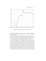
Figure 7.10 pictures the CPI inflation rate for Japan. We see that deflation
set in after 1995, with a slight recovery from deflation in 1998.
Figure 7.11 pictures the output gap, while Figures 7.12 and 7.13 contain

the rate of growth of the import price index and unit labor costs. We see
that the collapse of excess demand, measured as a positive output gap, goes
hand-in-hand with the onset of deflation. Unit labor costs also switched
from positive to negative growth rate at the same time. However there is
no noticeable collapse in the import price index at the time of the deflation.
1975 1980 1985 1990 1995 2000 200
5
−0.04
0
0.02
−0.02
0.04
0.06
0.08
0.1
FIGURE 7.11. Output gap: Japan
1975 1980 1985 1990 1995 2000 2005
−0.6
−0.4
−0.2
0
0.2
0.4
0.6
0.8
FIGURE 7.12. Rate of growth of import prices: Japan
186 7. Inflation and Deflation: Hong Kong and Japan
1975 1980 1985 1990 1995 2000 2005
0
0.02

−0.02
0.04
−0.04
0.06
0.08
0.1
FIGURE 7.13. Rate of growth of unit labor costs: Japan
Figure 7.14 pictures the rate of growth of two financial market indicators:
the Nikkei index and the land price index. We see that the volatility of the
rate of growth of the Nikkei index is much greater than that of the land
price index.
Figure 7.15 pictures the evolution of two indicators of monetary policy:
the Gensaki interest rate and the rate of growth of bank lending. The
Gensaki interest rate is considered the main interest for interpreting the
stance of monetary policy in Japan. The rate of growth of bank lending is,
of course, an indicator of how banks may thwart expansionary monetary
policy by reducing their lending. We see the sharp collapse of the rate
of growth of bank lending at about the same time the Bank of Japan
raised the interest rates at the beginning of the 1990s. The well-documented
action was an attempt by the Bank of Japan to burst the bubble in the
stock market. Figure 7.14, of course, shows that the Bank of Japan did
indeed succeed in bursting this bubble. After that, however, overall demand
showed a steady decline.
Table 7.6 gives a statistical summary of the data we have examined.
The highest volatility rates (measured by the standard deviations of the
1975 1980 1985 1990 1995 2000 2005
−0.8
−0.6
−0.4
−0.2

0
0.2
0.4
0.6
Rate of Growth
of Nikkei Index
Rate of Growth of
Land Price Index
FIGURE 7.14. Financial market indicators: Japan
1975 1980 1985 1990 1995 2000 2005
−0.04
−0.02
0
0.02
0.04
0.06
0.08
0.1
0.12
Gensaki
Interest
Rate
Rate of Growth of
Bank Lending
FIGURE 7.15. Monetary policy indicators: Japan
188 7. Inflation and Deflation: Hong Kong and Japan
TABLE 7.6. Statistical Summary of Data
Inflation Gensaki Y-gap Imp Ulo Lpi Spi Loan
Growth Growth Growth Growth Growth
Mean 0.034 0.052 0.000 0.016 0.004 0.035 0.068 0.077

Std. Dev. 0.043 0.036 0.017 0.193 0.014 0.074 0.202 0.054
Correlation Matrix
Inflation Gensaki Y-gap Imp Ulo Lpi Spi Loan
Growth Growth Growth Growth Growth
Inflation 1.000
Gensaki 0.607 1.000
Y-gap −0.211 0.309 1.000
Imp Growth 0.339 0.550 0.225 1.000
Ulo Growth 0.492 0.198 −0.052 0.328 1.000
Lpi Growth 0.185 0.777 0.591 0.345 −0.057 1.000
Spi Growth −0.069 −0.011 −0.286 −0.349 −0.176 0.081 1.000
Loan Growth 0.489 0.823 0.310 0.279 −0.016 0.848 0.245 1.000
annualized quarterly data) are for the rates of growth of the share market
and import price indices.
Table 7.6 shows that the highest correlation of inflation is with the
Gensaki rate, but that it is positive rather than negative. This is another
example of the well-known price puzzle, recently analyzed by Giordani
(2001). This puzzle is also a common finding of linear vector autoregressive
(VAR) models, which show that an increase in the interest rate has positive,
rather than negative, effects on the price level in impulse-response analysis.
Sims (1992) proposed that the cause of the prize puzzle may be unobserv-
able contemporaneous supply shocks. The policymakers observe the shock
and think it will have positive effects on inflation, so they raise the interest
rates in anticipation of countering higher future inflation. Sims found that
this puzzle disappears in U.S. data when we include a commodity price
index in a more extensive VAR model.
Table 7.6 also shows that the second and third highest correlations of
inflation are with unit labor costs and bank lending, followed by import
price growth. The correlations of inflation with the share-price growth rate
and the output gap are negative but insignificant.

Finally, what is most interesting from the information given in Table 7.6
is the very high correlation between the growth rate of bank lending and
the growth rate of the land price index, not the growth rate of the share
price index. It is not clear which way the causality runs: does the collapse
of land prices lead to a fall in bank lending, or does the collapse of bank
lending lead to a fall in land prices?
7.2 Japan 189
TABLE 7.7. Granger Test of Causality: LPI and Loan Growth
Loan Growth Does Not LPI Growth Does Not
Cause LPI Growth Cause Loan Growth
F-Statistic 2.429 3.061
P-Value 0.053 0.020
In Japan, the story is different: banking credit and land prices show
bidirectional causality or feedback. The collapse of land prices reduces bank
lending, but the collapse of bank lending also leads to a fall in land prices.
Table 7.7 gives the joint-F statistics and the corresponding P-values for a
Granger test of causality. We see that the results are somewhat stronger for
a causal effect from land prices to loan growth. However, the P-value for
causality from loan growth to land price growth is only very slightly above
5%. These results indicate that both variables have independent influences
and should be included as financial factors for assessing the behavior of
inflation.
7.2.2 Model Specification
We use the same model specification for the Hong Kong deflation as in
7.1.2 with two exceptions: we do not use a price gap variable measur-
ing convergence with mainland China, and we include both the domestic
Gensaki interest rate and the rate of growth of bank lending as further
explanatory variables for the evolution of inflation. As before, we forecast
over a one-year horizon, and all rates of growth are measured as annual
rates of growth, with ∆

h
x
t
= x
t
− x
t−h
and with h =4.
7.2.3 In-Sample Performance
Figure 7.16 pictures the in-sample performance of the three models. The
solid curve is for the error path of the linear model while similar dashed
and dotted paths are the errors for alternative STRS and NNRS models.
Both alternatives improve upon the performance of the linear model.
Adding a bit of complexity greatly improves the statistical in-sample fit.
Table 7.8 gives the in-sample diagnostic statistics of the three models.
We see that the STRS and NNRS models outperform the linear model,
not only on the basis if goodness-of-fit measures, but also on specification
tests. We can reject neither serial independence in the residuals nor the
squared residuals for both alternative models. Similarly, we cannot reject
normality in the residuals of both alternatives to the linear model. Finally,
the Brock-Deckert-Scheinkman and Lee-White-Granger tests show there is
very little or no evidence of neglected nonlinearity in the NNRS model.
190 7. Inflation and Deflation: Hong Kong and Japan
1975 1980 1985 1990 1995 2000 200
5
−0.08
−0.06
−0.04
−0.02
0

0.02
0.04
0.06
Linear
STRS
NNRS
FIGURE 7.16. In-sample paths of estimation errors
The information from Table 7.8 gives strong support for abandoning a
linear approach for understanding inflation/deflation dynamics in Japan.
7.2.4 Out-of-Sample Performance
Figure 7.17 gives the out-of-sample error paths of the three models. The
solid curve is for the linear prediction errors, the dashed path is for the
STRS prediction errors, and the dotted path is for the NNRS errors. We
see that the NNRS models outperforms both the STRS and linear models.
What is of interest, however, is that all three models generate negative
prediction errors in 1997, the time of the onset of the Asian crisis. The
models’ negative errors, in which the errors represent differences between
the actual and predicted outcomes, are indicators that the models do not
incorporate the true depth of the deflationary process taking place in Japan.
Table 7.9 gives the out-of-sample test statistics of the three models. We
see that the NNRS model has a much higher success ratio (in terms of
percentage correct sign predictions of the dependent variable), and outper-
forms the linear model as well as the STRS model in terms of the root
mean squared error statistic. The Diebold-Mariano statistics indicate that
7.2 Japan 191
TABLE 7.8. In-Sample Diagnostics of Alternative Models (Sample 1978–2002,
Quarterly Data)
Diagnostics Models
Linear STRS NNRS
SSE 0.023 0.003 0.003

RSQ 0.240 0.900 0.910
HQIF −315.552 −466.018 −467.288
LB* 0.067 0.458 0.681
ML* 0.864 0.254 0.200
JB* 0.002 0.172 0.204
EN* 0.531 0.092 0.084
BDS* 0.012 0.210 0.119
LWG 484 56 3
*: prob value
Note:
SSE: Sum of squared errors
RSQ: R-squared
HIQF: Hannan-Quinn information criterion
LB: Ljung-Box Q statistic on residuals
ML: McLeod-Li Q statistic on squared residuals
JB: Jarque-Bera statistic on normality of residuals
EN: Engle-Ng test of symmetry of residuals
BDS: Brock-Deckert-Scheinkman test of nonlinearity
LWG: Lee-White-Granger test of nonlinearity
the NNRS prediction errors are statistically different from the linear model.
However, the STRS prediction errors are not statistically different from
either the linear or the NNRS model.
7.2.5 Interpretation of Results
The partial derivatives of the model for Japan, as well as the tests of
significance based on bootstrapping methods, appear in Table 7.10. We see
that the only significant variables determining future inflation are current
inflation, the interest rate, and the rate of growth of the land price index.
The output gap is almost, but not quite, significant. Unit labor costs and
the Nikkei index are both insignificant and have the wrong sign.
The significant but wrong sign of the interest rate may be explained by

the fact that the Bank of Japan is constrained by the zero lower bound
of interest rates. They were lowering interest rates, but not enough during
the period of deflation, so that real interest rates were in fact increasing.
We see this in Figure 7.18.
192 7. Inflation and Deflation: Hong Kong and Japan
1988 1990 1992 1994 1996 1998 2000 2002
−0.04
−0.03
−0.02
−0.01
0
0.01
0.02
0.03
0.04
0.05
Linear
NNRS
STRS
FIGURE 7.17. Out-of-sample prediction errors
TABLE 7.9. Out-of-Sample Forecasting Accuracy
Diagnostics Models
Linear STRS NNRS
RMSQ 0.018 0.017 0.013
SR 0.511 0.489 0.644
Diebold-Mariano Linear vs. STRS Linear vs. NNRS STRS vs. NNRS
Test
DM-1* 0.276 0.011 0.233
DM-2* 0.304 0.016 0.271
DM-3* 0.310 0.007 0.285

DM-4* 0.306 0.001 0.289
DM-5* 0.301 0.001 0.288
*: prob value
RMSQ: Root mean squared error
SR: Success ratio on sign correct sign predictions
DM: Diebold-Mariano test
(correct for autocorrelation, lags 1–5)
7.2 Japan 193
TABLE 7.10. Partial Derivatives of NNRS Model
Period Arguments
Inflation Interest Import Lending Nikkei Land Price Output Unit Labor
Rate Price Growth Index Index Gap Costs
Mean 0.182 0.212 0.113 0.025 −0.088 0.122 0.015 −0.075
1978 0.190 0.217 0.123 0.039 −0.089 0.112 0.019 −0.092
1995 0.183 0.212 0.114 0.026 −0.088 0.121 0.015 −0.077
2002 0.181 0.211 0.112 0.023 −0.087 0.124 0.015 −0.074
Statistical Significance of Estimates
Period Arguments
Inflation Interest Import Lending Nikkei Land Price Output Unit Labor
Rate Price Growth Index Index Gap Costs
Mean 0.000 0.000 0.859 0.935 0.356 0.000 0.149 1.000
1978 0.000 0.000 0.819 0.933 0.288 0.000 0.164 1.000
1995 0.000 0.000 0.840 0.931 0.299 0.000 0.164 1.000
2002 0.000 0.000 0.838 0.935 0.293 0.000 0.149 1.000
1975 1980 1985 1990 1995 2000 2005
0
0.02
−0.02
0.04
−0.04

0.06
0.08
0.1
Real Interest
Rates
Inflation
FIGURE 7.18. Real interest rates and inflation in Japan
194 7. Inflation and Deflation: Hong Kong and Japan
The fact that the land price index is significant while the Nikkei index is
not can be better understood by looking at Figure 7.14. The rate of growth
has shown a smooth steady decline, more in tandem with the inflation
process than with the much more volatile Nikkei index.
Table 7.11 gives the corresponding sets of partial derivatives and tests
of significance from the STRS model. The only difference we see from the
NNRS model is that the output gap variable is also significant.
Figure 7.19 pictures the evolution of inflation and the transition neurons
of the two models. As in the case of Hong Kong, the STRS transition neu-
ron gives more information, showing that the likelihood of remaining in
the inflation state is steadily decreasing as inflation switches to deflation
after 1995. The NNRS model’s transition neuron shows little or no action,
remaining close to 0.5. The result indicates that the NNRS model outper-
forms the linear and STRS model not by picking up a regime change per
se but rather by approximating nonlinear processes in the overall inflation
process.
The fact that bank lending does not appear as a significant determi-
nant of inflation (while output gap does — at least in the STRS model)
does not mean that bank lending is not important. Table 7.12 pictures the
results of a Granger causality test between the output gap and the rate of
growth of bank lending in Japan. We see strong evidence, at the 5% level
TABLE 7.11. Partial Derivatives of STRS Model

Period Arguments
Inflation Interest Import Lending Nikkei Land Price Output Unit Labor
Rate Price Growth Index Index Gap Costs
Mean 0.149 0.182 0.054 −0.094 −0.032 0.208 0.028 −0.079
1978 0.138 0.163 0.055 −0.096 −0.032 0.232 0.030 −0.080
1995 0.138 0.163 0.055 −0.096 −0.032 0.232 0.030 −0.080
2002 0.133 0.156 0.056 −0.096 −0.032 0.242 0.030 −0.080
Statistical Significance of Estimates
Period Arguments
Inflation Interest Import Lending Nikkei Land Price Output Unit Labor
Rate Price Growth Index Index Gap Costs
Mean 0.006 0.000 0.695 1.000 0.398 0.000 0.095 1.000
1978 0.006 0.000 0.695 1.000 0.398 0.000 0.095 1.000
1995 0.006 0.000 0.615 1.000 0.394 0.000 0.088 0.863
2002 0.002 0.000 0.947 1.000 0.739 0.000 0.114 1.000
7.2 Japan 195
1975 1980 1985 1990 1995 2000 200
5
0
0.02
−0.02
0.04
−0.04
0.06
0.08
1975 1980 1985 1990 1995 2000 200
5
0.46
0.48
0.5

0.52
0.54
0.56
0.58
Inflation
Transition Neurons
STRS Model
NNRS Model
FIGURE 7.19. Regime transitions in STRS and NNRS models
TABLE 7.12. Ganger Test of Causality: Loan Growth and the Output Gap
Hypothesis
Loan Growth Does Not Output Gap Does Not
Cause the Output Gap Cause Loan Growth
F-Statistic 2.52.4
P-Value 0.049 0.053
of significance, that the rate of growth of bank loans is a causal factor for
changes in the output gap. There is also evidence of reverse causality, from
the output gap to the rate of growth of bank lending, to be sure. These
results indicate that a reversal in bank lending will improve the output
gap, and such an improvement will call forth more bank lending, leading,
in turn, in a virtuous cycle, to further output-gap improvement and an
escape from the deflationary trap in Japan.
196 7. Inflation and Deflation: Hong Kong and Japan
7.3 Conclusion
The chapter illustrates how neural network regime switching models help
explain the evolution of inflation and deflation in Japan and Hong Kong.
The results for Hong Kong indicate that external prices and residential
property prices are the most important factors underlying inflationary
dynamics, whereas for Japan, interest rates and excess demand (prox-
ied by the output gap) appear to be more important. These results are

consistent with well-known stylized facts about both economies. Hong
Kong is a much smaller and more highly open economy than Japan, so
that the evolution of international prices and nontraded prices (prox-
ied by residential property prices) would be the driving forces behind
inflation. For Japan, a larger and less open economy, we would expect
policy variables and excess demand to be more important factors for
inflation.
Clearly, there are a large number of alternative nonlinear as well as neural
network specifications for approximating the inflation processes of different
countries. We used a regime switching approach since both Hong Kong and
Japan have indeed moved from inflationary to deflationary regimes. But for
most countries, the change in regime may be much different, such as an
implicit or explicit switch to inflation-targets for monetary policy. These
types of regime switches cannot be captured as easily as the switch from
inflation to deflation.
Since inflation is of such central importance for both policymakers and
decision makers in business, finance, and households, it is surprising that
more work using neural networks has not been forthcoming. Chen, Racine,
and Swanson (2001) have used a ridgelet neural network for forecasting
inflation in the United States. McNelis and McAdam (2004) used a thick
model approach (combining forecasts of different types of neural nets) for
both the Euro Zone and the United States. Both of these papers show the
improved forecasting performance from neural network methods. Hopefully,
more work will follow.
7.3.1 MATLAB Program Notes
The same programs used in the previous chapter were used for
the inflation/deflation studies. The data are given in honkonginfla-
tion
may2004 run8.mat and japdata may2004 run3.mat for Hong Kong
and Japan.

7.3.2 Suggested Exercises
The reader is invited to use data from other countries to see how well
the results from Japan or Hong Kong carry over to countries that did not
7.3 Conclusion 197
experience deflation as well as inflation. However, the threshold would have
to be changed from zero to a very low positive inflation level. What would
be of interest is the role of residential property prices as a key variable
driving inflation.