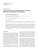
Báo cáo hóa học: " Research Article A Framework for the Assessment of Temporal Artifacts in Medium Frame-Rate Binary Video Halftones" pot

Hindawi Publishing Corporation
EURASIP Journal on Image and Video Processing
Volume 2010, Article ID 625191, 11 pages
doi:10.1155/2010/625191
Research Article
A Framework for the Assessment of Temporal Artifacts in
Medium Frame-Rate Binary Video Halftones
Hamood-Ur Rehman and Brian L. Evans
Wireless Networking and Communications Group, Department of Electrical and Computer Engineering,
The University of Texas at Aust in, Austin, TX 78712, USA
Correspondence should be addressed to Hamood-Ur Rehman,
Received 1 May 2010; Accepted 2 August 2010
Academic Editor: Zhou Wang
Copyright © 2010 H. Rehman and B. L. Evans. This is an open access article distributed under the Creative Commons Attribution
License, which permits unrestricted use, distribution, and reproduction in any medium, provided the original work is properly
cited.
Display of a video having a higher number of bits per pixel than that available on the display device requires quantization prior to
display. Video halftoning performs this quantization so as to reduce visibility of certain artifacts. In many cases, visibility of one
set of artifacts is decreased at the expense of increasing the visibility of another set. In this paper, we focus on two key temporal
artifacts, flicker and dirty-window-effect, in binary video halftones. We quantify the visibility of these two artifacts when the video
halftone is displayed at medium frame rates (15 to 30 frames per second). We propose new video halftoning methods to reduce
visibility of these artifacts. The proposed contributions are (1) an enhanced measure of perceived flicker, (2) a new measure of
perceived dirty-window-effect, (3) a new video halftoning method to reduce flicker, and (4) a new video halftoning method to
reduce dirty-window-effect.
1. Introduction
Bit-depth reduction must be performed when the number of
bits/pixel (bit-depth) of the original video data is higher than
the bit-depth available on the display device. Halftoning is
a process that can perform this quantization. The original,
full bit-depth video is called the continuous-tone video, and
the reduced bit-depth video is called the halftone video. Bit-

depth reduction results in quantization artifacts.
Binary halftone videos can suffer from both spatial and
temporal artifacts. In the case of binary halftone videos
produced from grayscale continuous-tone videos, there are
two key temporal artifacts. These temporal artifacts are
flicker and dirty-window-effect (DWE). Of these two tem-
poral artifacts, halftone flicker has received more attention
in publications on video halftoning [1–5]. Hilgenberg et
al. briefly discuss the DWE artifact in [6]. They have,
however, not used the term dirty-window-effect to refer to
this particular artifact.
The DWE refers to the temporal artifact that gives a
human viewer the perception of viewing objects, in the
halftone video, through a “dirty” transparent medium, such
as a window. The artifact is usually disturbing to the viewer
because it gives the perception as if a pattern were laid on
top of the actual video. Like other artifacts, dirty-window-
effect contributes to a degraded viewing experience of the
viewer. Although this artifact is known and has been referred
to in the published literature [6], as far as we know, a
quantitative perceptual criteria to assess this artifact has not
been published. The artifact has been evaluated qualitatively
in [6].
In contrast to DWE, which is observed due to binary
pixels not toggling in enough numbers in response to a
changing scene, flicker is typically observed due to too many
binary pixels toggling their values in spatial areas that do not
exhibit “significant” perceptual change between successive
(continuous-tone) frames. Depending on the type of display,
flicker can appear as full-field flicker or as scintillations. As

a temporal artifact, halftone flicker can appear unpleasant
to a viewer. On some devices, it can also result in higher
power consumption [7]. Moreover, if the halftone video is
to be compressed for storage or transmission, higher flicker
can reduce the compression efficiency [2, 3]. Evaluation of
flicker has been discussed in [2–5]. Flicker has been referred
2 EURASIP Journal on Image and Video Processing
to as high frequency temporal noise in [2].Arecentapproach
to form a perceptual estimate of flicker has been discussed in
[1].
For reasons discussed above, it is desirable to reduce these
temporal artifacts in the halftone videos. Therefore, per-
ceptual quantitative measures for evaluating these artifacts
are desirable. Quantitative assessment of temporal artifacts
can facilitate comparison of binary halftone videos produced
using different algorithms. Temporal artifact quality assess-
ment criteria can also be combined with the assessment of
spatial artifacts to form an overall quality assessment criteria
for binary halftone videos. Video halftoning algorithm
design can benefit from the temporal artifact evaluation
criteria presented in this paper. The perception of temporal
artifacts is dependent on the frame-rate at which the halftone
video is viewed. For example, for medium frame rate (15 to
30 frames per second) binary halftone videos, flicker between
successive halftone frames will correspond to temporal
frequencies at which the human visual system (HVS) is
sensitive [8].
In this paper, we present a framework for the quantitative
evaluation of the temporal artifacts in medium frame rate
binary halftone videos produced from grayscale continuous-

tone videos. We utilize the proposed quality assessment
framework to design video halftoning algorithms. The pro-
posed contributions of this paper include (1) an enhanced
measure of perceived flicker, (2) a new measure of perceived
dirty-window-effect, (3) a new video halftoning method to
reduce flicker, and (4) a new video halftoning method to
reduce dirty-window-effect.
The rest of the paper is organized as follows. Flicker and
dirty-window-effect in binary halftone videos are discussed
in detail in Section 2. Section 3 presents the proposed
technique to assess temporal artifacts. Section 3 also presents
halftoning algorithms that reduce temporal artifacts based
on the proposed quality assessment techniques. The paper
concludes with a summary of the proposed contributions in
Section 4.
2. Flicker and Dirty-Window-Effect
As discussed in the previous section, dirty-window-effect
refers to the temporal artifact that causes the illusion of
viewing the moving objects, in the halftone video, through
a dirty window. In medium frame-rate binary halftone
videos, the perception of dirty-window-effect depends pri-
marily on both the continuous-tone and the corresponding
halftone videos. Consider two successive continuous-tone
frames and their corresponding halftone frames. Assume
that some objects that appear in the first continuous-
tone frame change their spatial position in the second,
successive, continuous-tone frame, but the corresponding
halftone frames do not “sufficiently” change in their halftone
patterns at the spatial locations where the continuous-tone
frames changed. When each of the two halftone frames

is viewed independently, it represents a good perceptual
approximation of its corresponding continuous-tone frame.
However, when the two halftone frames are viewed in
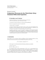
Figure 1: Frame 1 of the caltrain sequence.
Figure 2: Frame 1 of the caltrain sequence halftoned using
Ulichney’s 32
×32 void-and-cluster mask [9].
a sequence, if the change in their binary patterns does
not “sufficiently” reflect the corresponding change in the
continuous-tone frames, the halftone video can suffer from
perceivable dirty-window-effect. DWE should not be visible
if the successive continuous-tone frames are identical.
We now present an example to illustrate the point
discussed in the paragraph above. For this illustration, each
frame of the standard caltrain sequence [10] was indepen-
dently halftoned using Ulichney’s 32-by-32 void-and-cluster
mask [9]. Figures 1 and 2 show the first continuous-tone
frame and first halftone frame, respectively, of the caltrain
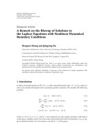
sequence. Figures 3 and 4 show the second continuous-
tone frame and second halftone frame, respectively. Figure 5
shows the absolute difference of the first two (grayscale)
continuous-tone frames. The brighter regions in this figure
represent spatial locations where the two successive frames
differed in luminance. Figure 6 shows the absolute difference
image of the halftone frames depicted in Figures 2 and 4.The
dark pixels in this image are the pixels that have identical
EURASIP Journal on Image and Video Processing 3
Figure 3: Frame 2 of the caltrain sequence.
Figure 4: Frame 2 of the caltrain sequence halftoned using
Ulichney’s 32

×32 void-and-cluster mask [9].
values in the, successive, halftone frames. Note that locations
of some of these dark pixels overlap with locations that
represent change of scene (due to moving objects or due to
camera motion) in Figure 5. These are the spatial locations
where perception of DWE is very likely in the halftone video.
This was found to be the case when we viewed the halftone
sequence at frame rates of 15 and 30 frames-per-second (fps).
For comparison, Figure 7 shows absolute difference of the
first two frames halftoned using Gotsman’s technique [2],
which is an iterative halftoning technique. It can be seen
by comparing Figures 6 and 7 with Figure 5 that Gotsman’s
method [2] produces less DWE than the frame independent
void-and-cluster method. This was our observation when
these videos were viewed at frame rates of 15 fps and 30 fps.
Now, consider a scenario where the values of grayscale
pixels within a (spatial) region of a continuous-tone frame
are close to the values of the corresponding pixels in the next
(successive) continuous-tone frame. If such is the case, one
Figure 5: Absolute difference of frame 1 (Figure 1)andframe2
(Figure 3) of caltrain sequence.
Figure 6: Absolute difference of the halftone for frame 1 (Figure 2)
and frame 2 (Figure 4) of the caltrain sequence. White pixels
indicate a change in halftone value, that is, a bit flip. Halftoning
on frames 1 and 2 was performed by using Ulichney’s 32
×32 void-
and-cluster mask.
would expect the corresponding binary halftone frames to
have similar pixels values as well. However, it is possible that
although each of the corresponding binary halftone frame

is perceptually similar to its continuous-tone version, when
viewed in a sequence the two successive halftone frames
toggle their pixel values within the same spatial region. This
can result in the perception of flicker.
Assessment of halftone flicker has traditionally been done
by evaluating difference images [2, 5]. In this approach, abso-
lute pixel-by-pixel difference between two successive halftone
frames is evaluated. The resulting binary image, called the
difference image, shows locations where pixels toggled their
values. Figure 8 illustrates flicker in two successive frames
of a halftone video. This technique is feasible for evaluating
flicker,ifonlyafewdifference images are to be looked at.
This technique will prove to be not feasible for videos with
4 EURASIP Journal on Image and Video Processing
Figure 7: Absolute difference of frame 1 and frame 2 of caltrain
sequence halftoned using Gotsman’s iterative method.
Figure 8: Absolute difference image computed from frames 40 and
41 in the trevor sequence halftoned using frame-independent error
diffusion.
large number of frames. The technique is also not objective,
since visual inspection of the difference image is required.
Moreover, higher flicker will be depicted with this technique
whenever there is a scene change in the video. This should
be considered a false positive. At a scene change, the binary
patterns are expected to change quite a bit to reflect the
scene change. This does not mean higher flicker. At a scene
change, temporal masking effects of the HVS also need to be
taken into account [11]. Hsu et al. proposed a method based
on the difference image technique to provide a quantitative
assessment of flicker for the entire halftone sequence [3].

They have called their assessment measure average flicker
rate (AFR), which they compute by adding the “on” pixels in
the absolute difference image and then dividing the resulting
sum by the total number of pixels in the frame. AFR is
evaluated for all adjacent pairs of halftone frames and plotted
as a function of frame number to give the flicker performance
of the entire video. In this paper, for the evaluation of
halftone flicker, we modify the approach proposed in [1].
3. Proposed Technique
In this section, we propose a framework that can be
utilized to evaluate temporal artifacts in medium frame-
rate binary video halftones. We assume that each frame of
the halftone video is a good halftone representation of the
corresponding continuous-tone frame. This is, for example,
the case when each continuous-tone frame is halftoned
independently to produce the corresponding halftone frame.
The proposed quality evaluation framework also depends on
the continuous-tone video from which the halftone video has
been produced. Therefore, our quality assessment measure is
a full-reference (FR) quality assessment measure. Before we
proceed with the presentation of the proposed framework,
we describe some observations about binary halftone videos
as follows.
(1) Flicker and dirty-window-effect in a binary halftone
video represent local phenomena. That is, their
perception depends on both the temporal and spatial
characteristics of the halftone video. Thus, flicker
or DWE may be more observable in certain frames
and in certain spatial locations of those frames. In
our observation, the perception of DWE is higher

if the moving objects (or regions) are relatively flat.
This means that moving objects with higher spatial
frequencies (or with higher degree of contrast) are
less likely to cause the perception of DWE. Similarly,
the perception of flicker is higher if the similar cor-
responding spatial regions of two successive halftone
frames have higher low spatial frequency (or low
contrast) content. It is interesting to note that for
still image halftones, it has been reported that the
nature of dither is most important in the flat regions
of the image [12]. This phenomenon is due to the
spatial masking effects that hide the presence of
noise in regions of the image that have high spatial
frequencies or are textured.
(2) Due to temporal masking mechanisms of the human
visual system (HVS) [11, 13], the perception of both
flicker and DWE might be negligible at scene changes.
(3) Flicker and DWE are related. Reducing one arti-
fact could result in an increase of the other. If
halftone pixels toggle values between halftone frames
within a spatial area that does not change much
between continuous-tone frames, flicker might be
observed at medium frame rates. If they do not
toggle in spatial areas that change between successive
frames or exhibit motion, DWE might be observed.
To minimize both artifacts, a halftoning algorithm
should produce halftone frames that have their pixels
toggle values only in spatial regions that have a
perceptual change (due to motion, e.g.) between the
corresponding successive continuous-tone frames.

EURASIP Journal on Image and Video Processing 5
C
i−1
L
Scene cut
detection
SSIM
K
+
Q
C
i
Filter P
+
Artifact map
D
i−1
S
−
R
HVS
D
i
+
Figure 9: Graphical depiction of the halftone temporal artifact quality assessment framework.
Certain halftoning algorithms produce videos that
have high DWE but low flicker. An example is a
binary halftone video produced by using ordered-
dither technique on each grayscale continuous-tone
frame independently. Similarly, there are halftoning

algorithms that produce videos with high flicker but
low DWE. An example is a binary halftone video
produced by halftoning each grayscale continuous-
tone frame independently using Floyd and Steinberg
[14]errordiffusion algorithm.
The observations discussed above are reflected in the
design of the framework for evaluation of temporal artifacts,
which we introduce now. To facilitate the clarity of presen-
tation, we utilize the notation introduced in [1]. We adapt
that notation for the current context and have described it in
Ta bl e 1. Please refer to the notation in Ta bl e 1 regarding the
terminology used in the rest of this paper.
Let I be the total number of frames in V
c
.LetM be the
total number of pixel rows in each frame of V
c
, and let N be
thetotalnumberofpixelcolumnsineachframeofV
c
.
3.1. Halftone Dirty-Window-Effect Evaluation. It has been
explained in the previous section that dirty-window-effect
may be observed if, between successive frames of a halftone
video, the halftone patterns do not change sufficiently in
response to a changing scene in the continuous-tone video.
Based on our observations on DWE, note that DWE
i
(m, n)
is a function of C

d,i,i−1
(m, n), D
s,i,i−1
(m, n), and W
i
(m, n).
Therefore,
DWE
i
(
m, n
)
= f

C
d,i,i−1
(
m, n
)
, D
s,i,i−1
(
m, n
)
, W
i
(
m, n
)


.
(1)
Figure 10: Structural dissimilarity map of the first two frames of
the continuous-tone caltrain sequence.
For the ith halftone frame, we also define perceived average
dirty-window-effect as

DWE
i
=

m

n
DWE
i
(
m, n
)
M · N
. (2)
Perceptual dirty-window-effect Index DWE ofahalftone
video V
d
is defined as
DWE
=

i


DWE
i
(
I
−1
)
. (3)
Dirty-window-effect performance of individual halftone
frames can be represented as a plot of

DWE
i
against frame
6 EURASIP Journal on Image and Video Processing
Table 1: Notation.
C
i
: ith frame of continuous-tone (original) video, V
c
;
C
i
(m, n): pixel located at mth row and nth column of the continuous-tone frame C
i
;
C
s,i,j
(m, n): local similarity measure between continuous-tone frames C
i
and C

j
at pixel location (m,n);
C
s,i,j
: similarity map/image between continuous-tone frames C
i
and C
j
;
C
d,i, j
(m, n): local dissimilarity measure between continuous-tone frames C
i
and C
j
at pixel location (m,n);
C
d,i, j
: dissimilarity map/image between continuous-tone frames C
i
and C
j
;
D
i
: ith frame of halftoned video, V
d
;
D
i

(m, n): pixel located at mth row and nth column of the halftone frame D
i
;
D
s,i,j
(m, n): local similarity measure between halftone frames D
i
and D
j
at pixel location (m,n);
D
s,i,j
= similarity map/image between halftone frames D
i
and D
j
;
D
d,i, j
(m, n): local dissimilarity measure between halftone frames D
i
and D
j
at pixel location (m, n);
D
d,i, j
: dissimilarity map/image between halftone frames D
i
and D
j

;
DWE
i
(m, n): local perceived DWE measure at pixel location (m, n)intheith halftone frame (i ≥ 2);
DWE
i
: perceived DWE map/image at the ith halftone frame (i ≥ 2);

DWE
i
: perceived average DWE observed at the ith halftone frame (i ≥ 2);
F
i
(m, n): local perceived flicker measure at pixel location (m, n)intheith halftone frame (i ≥ 2);
F
i
: perceived flicker map/image at the ith halftone frame (i ≥ 2);

F
i
: perceived average flicker observed at the ith halftone frame (i ≥ 2).
W
i
(m, n): local contrast measure at pixel location (m, n)intheith continuous-tone frame;
W
i
: contrast map/image of C
i
;
V

c
: continuous-tone video;
V
d
: the corresponding halftone video.
Figure 11: Normalized standard deviation map of the second
continuous-tone frame of the caltrain sequence.
number. The DWE performance of the entire halftone video
is given by the single number DWE, the Perceptual DWE
Index. The framework introduced thus far is quite general.
We have not described the form of the function in (1). We
have also not described how to calculate the arguments of
this function. We provide these details next.
We now describe a particular instantiation of the
framework introduced before. DWE
i
(m, n), C
d,i,i−1
(m, n),
D
s,i,i−1
(m, n), and W
i
(m, n) constitute the maps/images
DWE
i
, C
d,i,i−1
, D
s,i,i−1

,andW
i
,respectively.Toevaluate
DWE
i
(m, n)in(1), we need the (local) contrast map of
C
i
, W
i
, dissimilarity map between continuous-tone frames
C
i
and C
i−1
, C
d,i,i−1
, and the similarity map between the
successive halftone frames D
i
and D
i−1
, D
s,i,i−1
.Wederive
C
d,i,i−1
from the Structural Similarity (SSIM) Index Map [15]
evaluated between the continuous-tone frames C
i

and C
i−1
.
We will denote this derived measure by SSIM
{C
i
, C
i−1
}.We
scale SSIM
{C
i
, C
i−1
} to have its pixels take values between 0
and 1 inclusive. For the dissimilarity map, we set
C
d,i,i−1
= 1 − SSIM{C
i
, C
i−1
}. (4)
For the similarity map, we set
D
s,i,i−1
=
(
1
−|D

i
−D
i−1
|
)
∗

p,(5)
where

p represents the point spread function (PSF) of the
HVS and
|D
i
− D
i−1
| represents absolute difference image
for successive halftone frames D
i
and D
i−1
. We are assuming
that the HVS can be represented by a linear shift-invariant
system [16]representedby

p. For the evaluation of

p,we
utilize Nasanen’s model [17] to form a model for HVS. The
pixel values of the map D

s,i,i−1
are between 0 and 1 inclusive.
We wan t W
i
torepresentanimagethathaspixelswithvalues
proportional to the local contrast content. Using W
i
,wewant
to give higher weight to spatial regions that are relatively
“flat.” We approximate the calculation of high local contrast
content by computing the local standard deviation. In this
operation, each pixel of the image is replaced by the standard
deviation of pixels in a 3
× 3 local window around the pixel.
The filtered (standard deviation) image is then normalized
EURASIP Journal on Image and Video Processing 7
0.08
0.09
0.1
0.11
0.12
0.13
0.14
0.15
0.16
0.17
DWE
0 5 10 15 20 25 30 35
Frame number
Void-and-cluster

Floyd-Steinberg error diffusion
Gotsman
Figure 12: Caltrain perceived average DWE in three different
halftone videos. The top curve is for (frame-independent) void-
and-cluster halftone. The middle curve is for halftone sequence
produced using (frame-dependent) Gotsman’s technique. The
lowest curve is for (frame-independent) Floyd and Steinberg error
diffusion halftone.
(via pixel wise division) by the mean image, which is also
computed by replacing each pixel by the mean value of pixels
in a 3
× 3 local window around the pixel. This gives us W
i
.
W
i
is further normalized to have pixel values between 0 and
1 inclusive. With these maps defined, we define (1)as
DWE
i
(
m, n
)
=
(
1
−SSIM{C
i
, C
i−1

}
(
m, n
))
·D
s,i,i−1
(
m, n
)
·
(
1
−W
i
(
m, n
))
.
(6)
Observe that DWE
i
(m, n) ∈ [0, 1]. This instantiation of
the DWE assessment framework is depicted in Figure 9.In
Figure 9, K, P,andR each has a value of
−1. L, Q,andS
have each a value of 1. The “Artifact Map” is DWE
i
.Eachof
its pixels, DWE
i

(m, n), is a product of three terms. At pixel
location (m,n), the first term measures the local dissimilarity
between the successive continuous-tone frames. A higher
value of the first term, (1
−SSIM{C
i
, C
i−1
}(m, n)), will mean
that the successive frames have a lower structural similarity
in a local neighborhood of pixels centered at pixel location
(m, n). This will in turn assign a higher weight to any DWE
observed. This reflects the fact that the “local” scene change
should result in higher perception of DWE if the halftone
pixels do not change “sufficiently” between the successive
frames. The second term, D
s,i,i−1
(m, n), depends on the
number of pixels that stayed the same in a neighborhood
around (and including) pixel location (m, n). It gives us
a measure of perceived DWE due to HVS filtering. Since
the HVS is modeled as a low-pass filter in this experiment,
D
s,i,i−1
(m, n) will have a higher value, if the “constant” pixels
form a cluster as opposed to being dispersed. The third term,
0.13
0.135
0.14
0.145

0.15
0.155
0.16
DWE
0 5 10 15 20 25 30 35
Frame number
Gotsman
Modified Gotsman
Figure 13: Caltrain DWE reduction: The bottom curve (dashed)
depicts perceptual improvement with modified Gotsman’s tech-
nique.
(1 − W
i
(m, n)), measures the low contrast content in a local
neighborhood centered at C
i
(m, n). A higher value of this
term will result in higher value of perceived DWE. This is to
incorporate spatial masking mechanisms of HVS. This term
can also be viewed as representing the amount of low spatial
frequency content. We incorporate the effect of scene changes
by setting DWE
i
to zero. This is where scene change detection
comes into play. This accounts for temporal masking effects.
Note that between successive continuous-tone frames C
i−1
and C
i
, a very low average value of SSIM{C

i
, C
i−1
} can
indicate a change of scene. Any scene change detection
algorithm can be utilized, however. For the results reported
in this paper, we determined scene changes in the videos
through visual inspection and manually set DWE
i
to zero at
frames where a scene change is determined to have occurred.
3.2. Experimental Results on DWE Assessment. We fir st
discuss the DWE evaluation results on the standard caltrain
sequence [10]. Figure 10 shows the dissimilarity map C
d,2,1
.
In this map/image, the brighter regions depict the areas
where the first two frames of the caltrain sequence are
structurally dissimilar. These are the regions where DWE is
likely to be observed, if the corresponding halftone pixels
do not “sufficiently” change between the successive halftone
frames. Figure 11 shows W
2
. In this map, the luminance
of a pixel is proportional to the local normalized standard
deviation in the image. Therefore, brighter regions in this
image correspond to areas where DWE is less likely to
be observed, if the corresponding halftone pixels do not
“sufficiently” change between the successive halftone frames.
The caltrain sequence [10] was halftoned using three

techniques. The first halftone sequence was formed by using
ordered-dither technique on each frame independently. The
8 EURASIP Journal on Image and Video Processing
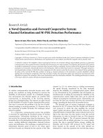
0
0.05
0.1
0.15
0.2
0.25
0.3
0.35
Perceived average flicker
0 20 40 60 80 100
Frame number
Void-and-cluster
Floyd-Steinberg error diffusion
Gotsman
Figure 14: Perceived Average Flicker evaluation in three different
halftones of the trevor sequence. Note the relatively higher value
of Perceived Average Flicker for (frame-independent) Floyd and
Steinberg error diffusion halftone video.
threshold array was formed by using a 32 × 32 void-
and-cluster mask [9]. The second sequence was formed
by halftoning the sequence using Gotsman’s technique [2].
The third halftone sequence was formed by halftoning each
frame independently using Floyd and Steinberg [14]error
diffusion. Figure 12 depicts DWE
i
plotted as a function of
frame number. According to this plot, the ordered-dither

halftone sequence has highest DWE. Gotsman’s technique
has relatively lower DWE, whereas the error diffusion based
halftone sequence has the lowest DWE. These results are
consistent with our visual inspection observations when the
sequence was played back at frame rates of 15 fps and 30 fps.
3.3. Validation of the DWE Assessment Framework. In this
section, we present our results on the validation of the
DWE assessment framework. To establish the validity of
the DWE assessment framework, we modified Gotsman’s
technique [2] such that our DWE assessment criteria were
incorporated while generating the halftone sequence. This
resulted in reduction of DWE in most halftone sequences.
We briefly describe Gotsman’s method to generate a halftone
video [2]. Gotsman’s method is geared towards reducing
flicker in halftone videos. The first frame of the halftone
video is generated by independently halftoning the cor-
responding continuous-tone frame. This is done via an
iterative technique which requires an initial halftone of the
image as the initial guess (or the starting point). The initial
halftone of the image is iteratively refined, via toggling the
bits, until a convergence criterion is met. The technique
results in achieving a local minimum of an HVS model-
based perceived error metric. For the first halftone frame,
the initial guess or the starting point can be any halftone
of the first continuous-tone frame. The starting point of
each subsequent frame is taken to be the preceding halftone
0
0.05
0.1
0.15

0.2
0.25
0.3
0.35
Perceived average flicker
0 20 40 60 80 100
Frame number
FDFSED
FIFSED
Figure 15: Perceived Average Flicker comparison between the
frame-dependent Floyd and Steinberg error diffusion (FDFSED)
and frame-independent Floyd and Steinberg error diffusion
(FIFSED) halftones of the trevor sequence. FDFSED results in
reduced flicker.
Continuous-tone pixel
(input)
+
+
Error
filter
+
−
Quantizer
Halftone pixel
(output)
Figure 16: Error diffusion for image halftoning.
frame. This causes each subsequent frame to converge to a
halftone which has a lot of pixels that do not toggle (with
respect to the preceding halftone frame), particularly when
there is no scene change. This results in producing halftone

frames that are temporally better correlated than those gen-
erally produced using a frame-independent (or intraframe)
approach. Our modification to this technique is as follows.
The first halftone frame is generated independently, just like
in Gotsman’s original technique. However, unlike Gotsman’s
technique [2], the initial guess for a subsequent frame is
not taken to be the preceding halftone frame in its entirety.
Instead, we only copy certain pixels from the previous frame.
In particular, to determine the initial guess of a frame (other
than the first frame), we produce a frame-independent
halftone of the corresponding continuous-tone frame using a
32
×32 void-and-cluster mask [9]. Then certain pixels of this
frame that meet a criteria, to be described next, are replaced
by pixels from the previous halftone frame. What pixels from
the previous frame need to be copied is determined based
on our DWE assessment technique. For the ith halftone
frame (i
≥ 2), D
i
, if a pixel location (m, n) in the initial
halftone is such that ((1
− SSIM{C
i
, C
i−1
}(m, n)) · (1 −
W
i
(m, n))) ≤ T, then the pixel from the preceding halftone

frame is copied into the initial halftone frame. Here T is a
EURASIP Journal on Image and Video Processing 9
Table 2: Evaluation of DWE Index. A higher value indicates higher
DWE.
Sequence Frames Resolution
DWE for
Gotsman’s
method
DWE for
modified
Gotsman’s
method
Caltrain 33 400 ×512 0.151 0.139
Tennis 150 240
×352 0.11 0.104
Garden 61 240
×352 0.18 0.171
Football 60 240
×352 0.113 0.127
Susie 75 240
×352 0.071 0.07
threshold that controls the amount of dirty-window-effect
reduction. With T
= 0.09, we produced the caltrain halftone
and compared it with Gotsman’s technique. Figure 13 depicts
the reduction in perceived DWE due to our modification
of Gotsman’s algorithm. Evaluation via visual inspection
confirmed the reduction in perceived DWE. Ta bl e 2 shows
more results for comparison of DWE Index, DWE,evaluation
for five different sequences [10]. The number of frames

reported in Ta bl e 2 is for 30 fps playback. Thus, Ta bl e 2 gives
DWE for 30 fps playback. For the modified method, T
=
0.09. Two points can be concluded based on the results
reported in the table. For most sequences, improvement in
the perception of DWE due to modified Gotsman’s method
is marginal. This was the case during our visual evaluation
of the sequences. One exception to this was the caltrain
sequence. This observation reinforces the fact that perception
of DWE is content dependent. It is interesting to note
that the modified Gotsman’s method actually produced the
football sequence with a slightly higher DWE.Thisisdue
to the fact that in the modified Gotsman’s method, it is the
content of the initial frame halftone that is controlled via
the modified method. However, since the method iteratively
improves the halftone frame, there is no explicit control on
how the halftone frame changes subsequently, and there is a
possibility for a scenario like this.
3.4. Halftone Flicker Evaluation. The development of frame-
work for halftone flicker evaluation will parallel the
approach, utilized above, for the evaluation of DWE, since
flicker and DWE are related artifacts. The development
presented below is based on the framework proposed in
[1]. Based on our discussion on flicker above, we note that
F
i
(m, n) is a function of C
s,i,i−1
(m, n), D
d,i,i−1

(m, n), and
W
i
(m, n). Thus,
F
i
(
m, n
)
= f

C
s,i,i−1
(
m, n
)
, D
d,i,i−1
(
m, n
)
, W
i
(
m, n
)

. (7)
For the ith halftone frame, Perceived Average Flicker is
defined as


F
i
=

m

n
F
i
(
m, n
)
M · N
. (8)
Perceptual Flicker Index F of a halftone video V
d
is defined
as
F =

i

F
i
(
I
−1
)
. (9)

Perceived Average Flicker

F
i
can be plotted (against frame
number) to evaluate flicker performance of individual
halftone frames. Perceptual Flicker Index F gives a single
number representing flicker performance of the entire
halftone video. Next, we present a particular instantiation of
the framework discussed thus far.
F
i
(m, n), C
s,i,i−1
(m, n), D
d,i,i−1
(m, n), and W
i
(m, n)con-
stitute the maps/images F
i
,C
s,i,i−1
, D
d,i,i−1
,andW
i
,respec-
tively. Therefore, to evaluate F
i

(m, n)in(7), we need the local
contrast map of C
i
, W
i
, similarity map between continuous-
tone frames C
i
and C
i−1
, C
s,i,i−1
, and the dissimilarity
map between the successive halftone frames D
i
and D
i−1
,
D
d,i,i−1
.WesetC
s,i,i−1
to be a map based on the Structural
Similarity (SSIM) Index Map [15] evaluated between the
continuous-tone frames C
i
and C
i−1
.Thiswillbedenoted
by SSIM

{C
i
, C
i−1
}. SSIM{C
i
, C
i−1
} is scaled to have its pixels
values between 0 and 1 inclusive. For the dissimilarity map,
we set
D
d,i,i−1
=
(
|D
i
−D
i−1
|
)
∗

p, (10)
where

p represents the point spread function (PSF) of
the HVS. This is based on the assumption that the HVS
can be represented by a linear shift-invariant system [16]
represented by


p. D
d,i,i−1
canhaveitspixelstakevalues
between 0 and 1 inclusive. W
i
is evaluated exactly as in the
case of DWE, already described in Section 3.1.Wedefine(7)
as
F
i
(
m, n
)
= SSIM{C
i
, C
i−1
}
(
m, n
)
·D
d,i,i−1
(
m, n
)
·
(
1

−W
i
(
m, n
))
.
(11)
Note that F
i
(m, n) ∈ [0, 1]. This instantiation of the
flicker assessment framework is depicted in Figure 9.In
Figure 9, K, Q,andR each have a value of 1. L,andS
have each a value of 0. P has a value of
−1. The “Artifact
Map” is F
i
. F
i
(m, n) has the form described in [1]. We do
evaluate W
i
differently in this paper. For clarity, we repeat
the description of F
i
(m, n)asprovidedin[1]. F
i
(m, n)is
a product of three terms. At pixel location (m, n), the first
term measures the local similarity between the successive
continuous-tone frames. A higher value of the first term,

SSIM
{C
i
, C
i−1
}(m, n), will mean that the successive frames
have a higher structural similarity in a local neighborhood
of pixels centered at pixel location (m, n). This will in
turn assign a higher weight to any flicker observed. This
is desired because if the “local” scene does not change,
perception of any flicker would be higher. The second term,
D
d,i,i−1
(m, n), depends on the number of pixels that toggled
in a neighborhood around (and including) pixel location
(m, n).ItgivesusameasureofperceivedflickerduetoHVS
filtering. Since the HVS is modeled as a low pass filter in
this experiment, D
d,i,i−1
(m, n) will have a relatively higher
value, if the pixel toggles form a cluster as opposed to being
dispersed. The third term, (1
− W
i
(m, n)), measures the
low contrast content in a local neighborhood centered at
C
i
(m, n). A higher value of this term will result in higher
value of perceived flicker. Finally, we incorporate the effect

10 EURASIP Journal on Image and Video Processing
of scene changes by setting F
i
(m, n) to a low value (zero,
e.g.), if a scene change is detected between continuous-
tone frames C
i−1
and C
i
.Thisistoaccountfortemporal
masking effects. For the results reported in this paper, we
(manually) determined scene changes in the videos through
visual inspection and manually set F
i
to zero whenever
a scene change is determined to have occurred between
successive continuous-tone frames C
i−1
and C
i
.
3.5. Experimental Results on Flicker Assessment. Now we
discuss the flicker evaluation results on the standard trevor
sequence [10]. This sequence was halftoned using three
techniques. The first halftone sequence was formed by using
ordered-dither technique on each frame independently. The
threshold array was formed by using a 32
× 32 void-
and-cluster mask [9]. The second sequence was formed
by halftoning the sequence using Gotsman’s technique [2].

The third halftone sequence was formed by halftoning each
frame independently using Floyd and Steinberg [14]error
diffusion. Figure 14 depicts F
i
plotted as a function of frame
number. As you can see on this plot, the error diffusion-based
halftone sequence has higher flicker relative to the other two
compared halftone sequences. Authors’ visual evaluation of
the sequences played back at frame rates of 15 fps and 30 fps
revealed highest flicker in the sequences generated using
Floyd and Steinberg [14]errordiffusion.
3.6. Validation of the Flicker Assessment Framework. To
validate the flicker assessment framework proposed in this
paper, we will utilize the flicker assessment framework
to modify an existing video halftoning algorithm. If this
modification results in improvement of perceived flicker
at medium frame rates, then the proposed framework is
valid. This is the case as will be shown next. We modify
frame-independent Floyd and Steinberg error diffusion
algorithm to reduce flicker. As described before, frame-
independent Floyd and Steinberg error diffusion (FIFSED)
algorithm halftones each frame of the continuous-tone video
independently using Floyd and Steinberg error diffusion
[14] algorithm for halftone images. The general set up for
image error diffusion is shown in Figure 16. In this system,
each input pixel, from the continuous tone image, to the
quantizer is compared against a threshold to determine its
binary output in the halftoned image. We modify FIFSED
and introduce frame-dependence in the algorithm. The
modified algorithm will be called frame-dependent Floyd

and Steinberg error diffusion (FDFSED) algorithm. To
make the algorithm frame-dependent (or interframe), we
will incorporate threshold modulation for flicker reduction.
The idea of threshold modulation to reduce flicker was
originally conceived by Hild and Pins [4], and later used
in [5]. FDFSED works as follows. The first halftone frame
is generated by halftoning the first continuous-tone frame
using image error diffusion algorithm. In this algorithm,
the error diffusion quantization threshold is kept a constant
[14]. For the generation of subsequent halftone frames,
the quantization threshold is not constant. Instead, the
quantization threshold is modulated based on our flicker
Table 3: Evaluation of Flicker Index. A higher value indicates higher
flicker.
Sequence Frames Resolution F for FIFSED F FDFSED
Trevor 99 256 ×256 0.31 0.092
Garden 61 240
×352 0.232 0.134
Tennis 150 240
×352 0.344 0.096
Football 60 240
×352 0.329 0.123
Susie 75 240
×352 0.4 0.105
assessment framework. In the generation of each ith halftone
frame for (i
≥ 2), D
i
, the quantization threshold T
i

(m, n)for
a pixel location (m, n) is determined as follows:
T
i
(
m, n
)
=
⎧
⎪
⎪
⎪
⎪
⎪
⎪
⎪
⎪
⎨
⎪
⎪
⎪
⎪
⎪
⎪
⎪
⎪
⎩
0.5−Z ·
(
SSIM

{C
i
, C
i−1
}
(
m, n
)
·
(
1
−W
i
(
m, n
)))
if D
i−1
(
m, n
)
= 1,
0.5+Z
·
(
SSIM
{C
i
, C
i−1

}
(
m, n
)
·
(
1
−W
i
(
m, n
)))
if D
i−1
(
m, n
)
= 0.
(12)
As seen in (12), the amount of threshold perturba-
tion is determined by Z
· (SSIM{C
i
, C
i−1
}(m, n) · (1 −
W
i
(m, n))), where Z is a constant that controls the effect
of (SSIM

{C
i
, C
i−1
}(m, n) · (1 −W
i
(m, n))) on T
i
(m, n). The
threshold modulation is designed to reduce flicker in the
halftone video.
With Z
= 0.1in(12), we produced the trevor halftone
using FDFSED and compared with that generated using
FIFSED. Figure 15 depicts the reduction in perceived average
flicker in the trevor halftone produced using FDFSED. Visual
evaluation of the two halftone sequences (generated using
FIFSED and FDFSED methods) by the authors confirmed
the reduction in perceived average flicker in the sequence
generated using FDFSED method. Ta b le 3 shows more
results for comparison of flicker Index, F,evaluationforfive
different sequences [10]. For FDFSED algorithm, we used
Z
= 0.1in(12). Ta b le 3 shows the values of flicker Index, F
for the number of frames indicated in the table. The number
of frames reported in Ta bl e 3 is for 30 fps playback. Thus,
Ta bl e 3 gives F, for 30 fps playback. As can be seen in the
table, use of FDFSED resulted in significant reduction of
flicker in every halftone sequence. The results are consistent
with the authors’ visual evaluation at 30 frames per second.

4. Conclusion
In this paper, we presented a generalized framework for
the perceptual assessment of two temporal artifacts in
medium frame rate binary video halftones produced from
grayscale continuous-tone videos. The two temporal artifacts
discussed in this paper were referred to as halftone flicker and
halftone dirty-window-effect. For the perceptual evaluation
of each artifact, a particular instantiation of the generalized
framework, was presented and the associated results were
EURASIP Journal on Image and Video Processing 11
discussed. We also presented two new video halftoning
algorithms which were designed by modifying existing video
halftoning algorithms. The modifications were based on
the perceptual quality assessment framework and were thus
geared towards reducing the temporal artifacts. Results of
comparisons between the halftone videos generated using
the original and the modified algorithms were presented and
discussed.
References
[1] H. Rehman and B. L. Evans, “Flicker assessment of low-to-
medium frame-rate binary video halftones,” in Proceedings
of the IEEE Southwest Symposium on Image Analysis and
Interpretation (SSIAI ’10), pp. 185–188, Austin, Tex, USA, May
2010.
[2] C. Gotsman, “Halftoning of image sequences,” Visual Com-
puter, vol. 9, no. 5, pp. 255–266, 1993.
[3] C Y. Hsu, C S. Lu, and S C. Pei, “Video halftoning preserv-
ing temporal consistency,” in Proceedings of IEEE International
Conference on Multimedia and Expo (ICME ’07), pp. 1938–
1941, July 2007.

[4] H. Hild and M. Pins, “A 3-d error diffusion dither algorithm
for half-tone animation on bitmap screens,” in State-of-the-
Art in Computer Animation, pp. 181–190, Springer, Berlin,
Germany, 1989.
[5] Z. Sun, “Video halftoning,” IEEE Transactions on Image
Processing, vol. 15, no. 3, pp. 678–686, 2006.
[6] D. P. Hilgenberg, T. J. Flohr, C. B. Atkins, J. P. Allebach, and
C. A. Bouman, “Least-squares model-based video halftoning,”
in Human Vision, Visual Processing, and Digital Display V, vol.
2179 of Proceedings of SPIE, pp. 207–217, San Jose, Calif, USA,
February 1994.
[7] C Y. Hsu, C S. Lu, and S C. Pei, “Power-scalable multi-layer
halftone video display for electronic paper,” in Proceedings of
IEEE International Conference on Multimedia and Expo (ICME
’08), pp. 1445–1448, Hannover, Germany, June 2008.
[8] J. Robson, “Spatial and temporal contrast-sensitivity functions
of the visual system,” Journal of the Optical Society of America,
vol. 56, no. 8, pp. 1141–1142, 1966.
[9] R. A. Ulichney, “Void-and-cluster method for dither array
generation,” in Human Vision, Visual Processing, and Digital
Display IV, J. P. Allebach and B. E. Rogowitz, Eds., vol. 1913
of Proceedings of SPIE, pp. 332–343, San Jose, Calif, USA,
February 1993.
[10] R. P. I. Center for Image Processing Research,
/>[11] W. J. Tam, L. B. Stelmach, L. Wang, D. Lauzon, and P. Gray,
“Visual masking at video scene cuts,” in Human Vision, Visual
Processing, and Digital Display VI, vol. 2411 of Proceedings of
SPIE, pp. 111–119, February 1995.
[12] R. A. Ulichney, “Review of halftoning techniques,” in Color
Imaging: Device-Independent Color, Color Hardcopy, and

Graphic Arts V, vol. 3963 of Proceedings of SPIE, pp. 378–391,
San Jose, Calif, USA, January 2000.
[13] B. Girod, “The information theoretical significance of spatial
and temporal masking in video signals,” in Human Vision,
Visual processing, and Digital Display, vol. 1077 of Proceedings
of SPIE, pp. 178–187, 1989.
[14] R. Floyd and L. Steinberg, “An adaptive algorithm for spatial
grayscale,” in Proceedings of SID International Symposium,
Digest of Technical Papers, pp. 36–37, 1976.
[15] Z. Wang, A. C. Bovik, H. R. Sheikh, and E. P. Simoncelli,
“Image quality assessment: from error visibility to structural
similarity,” IEEE Transactions on Image Processing, vol. 13, no.
4, pp. 600–612, 2004.
[16] T.N.Pappas,J.P.Allebach,andD.L.Neuhoff, “Model-based
digital halftoning,” IEEE Signal Processing Magazine, vol. 20,
no. 4, pp. 14–27, 2003.
[17] R. Nasanen, “Visibility of halftone dot textures,”
IEEE Transac-
tions on Systems, Man and Cybernetics, vol. 14, no. 6, pp. 920–
924, 1984.