Báo cáo hóa học: " Research Article Red-Eyes Removal through Cluster-Based Boosting on Gray Codes" pptx

Hindawi Publishing Corporation
EURASIP Journal on Image and Video Processing
Volume 2010, Article ID 909043, 11 pages
doi:10.1155/2010/909043
Research Article
Red-Eyes Removal through Cluster-Based Boosting on Gray Codes
Sebastiano Battiato,
1
Giovanni Maria Farinella,
1
Mirko Guarnera,
2
Giuseppe Messina,
2
and Daniele Rav
`
ı
1
1
Image Processing Laboratory, Dipartimento di Matematica e Informatica, Universit
`
a di Catania, Viale A. Doria 6,
95125 Catania, Italy
2
Advanced System Technology, STMicroelectronics, Stradale Primosole 50, 95125 Catania, Italy
Correspondence should be addressed to Giovanni Maria Farinella,
Received 26 March 2010; Revised 2 July 2010; Accepted 29 July 2010
Academic Editor: Lei Zhang
Copyright © 2010 Sebastiano Battiato et al. This is an open access article distributed under the Creative Commons Attribution
License, which permits unrestricted use, distribution, and reproduction in any medium, provided the original work is properly
cited.

Since the large diffusion of digital camera and mobile devices with embedded camera and flashgun, the redeyes artifacts have de
facto become a critical problem. The technique herein described makes use of three main steps to identify and remove red eyes.
First, red-eye candidates are extracted from the input image by using an image filtering pipeline. A set of classifiers is then learned
on gray code features extracted in the clustered patches space and hence employed to distinguish between eyes and non-eyes
patches. Specifically, for each cluster the gray code of the red-eyes candidate is computed and some discriminative gray code bits
are selected employing a boosting approach. The selected gray code bits are used during the classification to discriminate between
eye versus non-eye patches. Once red-eyes are detected, artifacts are removed through desaturation and brightness reduction.
Experimental results on a large dataset of images demonstrate the effectiveness of the proposed pipeline that outperforms other
existing solutions in terms of hit rates maximization, false positives reduction, and quality measure.
1. Introduction
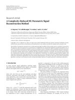
Red-eye artifact is caused by the flash light reflected off a
person’s retina (see Figure 1). This effect often occurs when
the flash light is very close to the camera lens, as in most
compact imaging devices. To reduce these artifacts, most
camerashaveared-eyeflashmodewhichfiresaseriesof
preflashes prior to picture capturing. Rapid preflashes cause
pupil contraction, thus, minimizing the area of reflection; it
does not completely eliminate the red-eye effect though it
reduces it. The major disadvantage of the preflash approach
is power consumption (e.g., flash is the most power-
consuming device of the camera). Besides, repeated flashes
usually cause uncomfortable feeling.
Alternatively, red eyes can be detected after photo acqui-
sition. Some photo-editing software makes use of red-eye
removal tools which require considerable user interaction.
To overcome this problem, different techniques have been
proposed in literature (see [1, 2] for recent reviews in
the field). Due to the growing interest of industry, many
automatic algorithms, embedded on commercial software,
have been patented in the last decade [3]. The huge variety of

approaches has permitted to explore different aspects of red-
eyes identification and correction. The big challenge now is
to obtain the best results with the minor number of visual
errors.
In this paper, an advanced pipeline for red-eyes detection
and correction is discussed. In the first stage, candidates rede-
yes patches are extracted from the input image through an
image filtering pipeline. This process is mainly based on a
statistical color model technique coupled with geometrical
constraints. In the second stage, a multimodal classifier,
obtained by using clustering and boosting on gray codes
features, is used to distinguish between true red-eyes patches
versus other patches. Once the red eyes are detected, a
correction technique based on desaturation and brightness
reduction is employed to remove the red-eyes artifact. The
proposed approach has been compared with respect to
existing solutions on proper collected dataset, obtaining
competitive results. One of the main contributions of the
2 EURASIP Journal on Image and Video Processing
α
β
Red eye cone
Eye
Figure 1: Flash-gun light cone generated by reflection off the retina.
If the angle α, representing the cone size, is greater than the angle β,
between the camera lens and the flash-gun, then the red-eye artifact
comes out.
present work is to demonstrate that better results are
achieved if the multimodally nature of candidates red-eyes as
well as the spatial information during classification task are

taken into account. To this aim, we have compared the pro-
posed cluster-based boosting, to standard boosting in both
cases, with and without considering spatial information.
The remainder of the paper is organized as follows.
Section 2 gives an overview of related works. Section 3
provides details of the proposed red-eyes removal pipeline.
Section 4 illustrates the experimental settings and the results
obtained using the presented technique. Finally, Section 5
concludes this paper with avenues for further research.
2. Related Works
Several studies have considered the problem of automatic
red-eyes removal. A pioneering technique for automatic red-
eye reduction was proposed by Patti et al. [4]. The technique
uses a nonstandard luminance-chrominance representation
to enhance the regions affected by the red-eye artifacts. After
the detection of an interesting block, thresholding operation
and a simple color replacement pipeline are employed to
remove the red eyes.
Battiato et al. [5] have proposed to deal with the problem
of red eye detection by using the bag-of-keypoints paradigm.
It involves extraction of local image features, quantization
of the feature space into a codebook through clustering,
and extraction of codeword distribution histograms. An
SVM classifier has been used to decide to which class each
histogram, thus each patch, belongs.
Gaubatz and Ulichney [6]proposedtoapplyaface
detector as first stage and then search for the eyes in the
candidate face regions by using constraints based on colors,
red variance, and glint. One of the drawbacks of such method
is the robustness with respect to the multimodality of the

face space with respect to poses (e.g., not always frontal and
upright). The redness of detected red eyes is attenuated with
a tapered color desaturation process.
Schildkraut and Gray [7] used an automatic algorithm
to detect pairs of eyes, which is restricted to near-frontal
face images. The pair verification technique was used to
reduce false positive. However, many photos have single
redeyes (e.g., face partially screened) that cannot be corrected
with this approach. Detected red eyes are removed blending
the corrected region with the neighborhood in order to
preserve the natural appearance of the eyes. Building on
[7], a combination of boosting classifiers has been proposed
by Ioffe[8]. Specifically, a boosting classifier was used to
discriminate between red-eyes versus other, and another
boosting classifier was used to detect faces in order to reduce
the false positives.
A two-stage algorithm was described by Zhang [9]. At the
first stage, red pixels are grouped, and a cascade of heuristic
algorithms to deal with color, size, and highlight is used to
decide whether the grouped region is red eye or not. At the
second stage, candidate red-eyes regions are checked by using
Adaboost classifier. Though highlight is useful for red-eyes
detection, some red eye with no highlight region may occur
when the eye direction does not face toward the camera/flash
light. Artifacts are corrected through brightness and contrast
adjustment followed by blending operation.
Luo et al. [10] proposed an algorithm that first uses
square concentric templates to assess the candidate red-eye
regions and then employs an Adaboost classifier coupled
with a set of adhoc selected Haar-like features for final

detection. Multiscale templates are used to deal with the scale
of red-eyes patches. For each scale, a thresholding process has
been used to determine which pixels are likely to be red-eye
pixels. The correction process is mainly based on adaptive
desaturation over the red-eye regions.
Petschnigg et al. [11] presented a red-eyes detection
technique based on changes of pupil color between the
ambient image and the flash image. The technique exploits
two successive photos taken with and without flash con-
sidered into YCbCr space to decorrelate luminance from
chrominance. The artifacts are detected by thresholding the
differences of the chrominance channels and using geometric
constraints to check size and shape of red regions. Detected
red eyes are finally corrected through thresholding operation
and the color replacement pipeline proposed in [4].
A wide class of techniques make use of geometric
constraints to restrict possible red-eye regions in com-
bination with reliable supervised classifiers for decision
making. Corcoran et al. [12] proposed an algorithm for
real-time detection of flash eye defects in the firmware of a
digital camera. The detection algorithm comprises different
substeps on Lab color space to segment artifacts regions that
are finally analyzed with geometric constraints.
The technique proposed by Volken et al. [13] detects the
eye itself by finding the suitable colors and shapes. They use
the basic knowledge that an eye is characterized by its shape
and the white color of the sclera. Combining this intuitive
approach with the detection of “skin” around the eyes, red-
eyes artifacts are detected. Correction is made through an
adhoc filtering process.

Safonov et al. [14] suggested a supervised approach
taking into account color information via 3D tables and
edge information via directional edge detection filters. In
the classification stage, a cascade of supervised classifiers has
been used. The correction consists in conversion of pixel to
gray color, darkening and blending with the initial image in
the YCbCr color space. The results were evaluated by using
an adhoc detection quality criterion.
Alternatively, an unsupervised method to discover red-
eye pixels was adopted by Ferman [15]. The analysis is
performed primarily in the hue-saturation-value (HSV)
EURASIP Journal on Image and Video Processing 3
color space. A flash mask, used to define the regions where
red-eye artifacts may be present, is first extracted from the
brightness component. Subsequent processing on the other
color components prunes the number of candidate regions
that may correspond to red eyes. Though the overall results
are satisfactory, this approach is not able to identify red-eyes
region outside the flash mask area (i.e.; a very common case).
The methods reviewed above comprise techniques pre-
sented in literature in the last decade. Other related
approaches are reviewed in [1–3].
3. Red-Eyes Detection and Correction
The proposed red-eyes removal pipeline uses three main
steps to identify and remove red-eyes artifacts. First, candi-
dates red-eyes patches are extracted, then they are they are
classified to distinguish between eyes and non-eyes patches.
Finally, correction is performed on detected red eyes. The
details of the three steps involved in the proposed pipeline
are detailed in the following subsections.

3.1. Red Patch Extraction. To extract the red-eyes candidates,
we first built a color model from the training set to detect pix-
els belonging to possible red-eyes artifacts. We constructed
red-eye-pixel and non-red-eye-pixel histogram models using
a set of pixels of the training images. Specifically, for each
image of the training set, the pixels belonging to red-eye
artifacts have been labeled as red-eye pixels (REP), whereas
the surrounding pixels within windows of fixed size have
been labeled as non-red-eye pixels (NREP). The labeled
pixels (in both RGB and HSV spaces) have been mapped
in a three-dimensional space C
1
× C
2
× C
3
obtained taking
into account the first three principal components of the
projection through principal component analysis [16]. By
using the principal component analysis, the original six-
dimensional space of each pixel, considered in both RGB and
HSV color domains, is transformed into a reduced three-
dimensional space maintaining as much of the variability
in the data as possible. This is useful to reduce the com-
putational complexity related to the space dimensionality.
We u sed a 3 D hi sto gr am w i th 6 4
× 64 × 64 bins in the
C
1
× C

2
× C
3
space. Since most of the sample pixels of
the training set lie within three standard deviations of the
mean, each component C
i
has been uniformly quantized in
64 values taking into account the range [
−3λ
i
,+3λ
i
], where
λ
i
is standard deviation of the ith principal component (i.e.,
the ith eigenvalue). The probability that a given pixel belongs
to the classes REP and NREP is computed as follows:
P
(
C
1
, C
2
, C
3
| REP
)
=

h
REP
[
C
1
, C
2
, C
3
]
T
REP
P
(
C
1
, C
2
, C
3
| NREP
)
=
h
NREP
[
C
1
, C
2

, C
3
]
T
NREP
(1)
where h
REP
[C
1
, C
2
, C
3
] is the red-eye-pixels count contained
in bin C
1
× C
2
× C
3
of the 3D histogram, h
NREP
[C
1
, C
2
, C
3
]is

the equivalent count for non-redeye pixels, T
REP
and T
NREP
are the total counts of red-eye pixels and non-red-eye pixels
respectively. We derive a red-eye-pixel classifier through the
standard likelihood ratio approach. A pixel is labeled red-eye
pixel if
P
(
C
1
, C
2
, C
3
| REP
)
>αP
(
C
1
, C
2
, C
3
| NREP
)
(2)
where α is a threshold which is adjusted to maximize correct

detection and minimize false positives. Note that a pixel is
assigned to NREP class when both probabilities are equal to
zero.
Employing such filtering, a binary map with the red
zones is derived. To remove isolated red pixels, a morphology
operation of closing is applied to this map. In our approach,
we have used the following 3
× 3 structuring element:
m
=
⎡
⎢
⎣
010
111
010
⎤
⎥
⎦
(3)
Once the closing operation has been accomplished, a search
of the connected components is achieved using a simple
scanline approach. Each group of connected pixels is ana-
lyzed making use of simple geometric constraints. As in
[13], the detected regions of connected pixels are classified
as possible red-eye candidates if the geometrical constraints
of size and roundness are satisfied. Specifically, a region of
connected red pixels is classified as possible red-eye candidate
if the following constraints are satisfied:
(i) the size S

i
of the connected region i is within the
range [Min
s
,Max
s
], which defines the allowable size
for eyes;
(ii) the binary roundness constraint R
i
of the connected
region i is verified as follows:
R
i
=
⎧
⎪
⎨
⎪
⎩
Tr ue ρ
i
∈

Min
ρ
,Max
ρ

; η

i
≤ Malx
η
; ξ
i
 0
False otherwise
(4)
where
(a) ρ
i
= (4π × A
i
)/P
2
i
is the ratio between the estimated
area A
i
and the perimeter P
i
of the connected region;
the more this value is near 1, the more the shape will
be similar to a circle;
(b) η
i
= max(Δ
(x
i
)

/Δ
(y
i
)
, Δ
(y
i
)
/Δ
(x
i
)
) is the distortion of
the connected region along the axes;
(c) ξ
i
= A
i
/(Δ
(x
i
)
Δ
(y
i
)
) is the filling factor; the more this
parameter is near 1, the more the area is filled.
The parameters involved in the aforementioned filtering
pipeline have been set through a learning procedure as

discussed in Section 4.
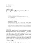
In Figure 2, all the involved steps in filtering pipeline
are shown. The regions of connected pixels which satisfy
the geometrical constraints are used to extract the red-eyes
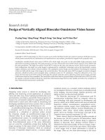
patches candidates from the original input image (Figure 3).
The derived patches are resembled to a fixed size (i.e., 30
×
30 pixels) and converted into gray code [17] for further
4 EURASIP Journal on Image and Video Processing
(a) Input image
(b) Red map
(c) Closing operation
(d) Final candidates
Figure 2: Filtering pipeline on (a)input image.
classification purpose (Figure 4). Gray code representation
allows to have a natural way (e.g., no strong transaction
between adjacent values) to pick up the underlying spatial
structures of a typical eye.
The gray levels of an m-bit gray-scale image (i.e., a color
channel in our case) are represented in the form of the base
2polynomial
a
m−1
2
m−1
+ a
m−2
2
m−2
+ ···+ a

1
2
1
+ a
0
2
0
(5)
Based on this property, a simple method of decomposing the
image into a collection of binary images is to separate the m
coefficients of the polynomial into m1-bit planes. The m-bit
Gray code (g
m−1
···g
2
, g
1
, g
0
) related to the polynomial in
(5) can be computed as follows:
g
i
=
⎧
⎨
⎩
a
i
⊕ a

i+1
0 ≤ i ≤ m − 2
a
m−1
i = m − 1
(6)
where
⊕ denotes the exclusive OR operation. This code has
the unique property that successive code words differ only
one bit position. Thus, small changes in gray level are less
likely to affect all m bit planes.
3.2. Red Patch Classification. The main aim of the classifi-
cation stage is the elimination of false positive red eyes in
the set of patches obtained performing the filtering pipeline
described in Section 3.1.
At this stage, we deal with a binary classification problem.
Specifically, we want to discriminate between eye versus
non-eye patches. To this aim, we employ an automatic
learning technique to make accurate predictions based on
past observations. The approach we use can be summarized
as follows: start by gathering as many examples as possible of
both eyes and non-eyes patches, next feed these examples,
together with labels indicating if they are eyes or not,
to a machine-learning algorithm which will automatically
produce a classification rule. Given a new unlabeled patch,
such a rule attempts to predict if it is eye or not.
Building a rule that makes highly accurate predictions
on new test examples is a challenging task. However, it is
not hard to come up with rough weak classifiers that are
only moderately accurate. An example of such a rule for the

problem under consideration is something like the following:
“If the pixel p located in the sclera region of the patch under
consideration is not white, then predict it is non-eye”. In
this case, such a rule is related to the knowledge that the
white region corresponding to the sclera should be present
in an eye patch. On the other hand, such a rule will cover
all possible non-eyes cases; for instance, it is correct to say
nothing about what to predict if the pixel p is white. Of
course, this rule will make predictions that are significantly
better than random guessing. The key idea is to find many
weak classifiers and combine them in a proper way deriving
a single strong classifier.
Among other, Boosting [18–20] is one of the most
popular procedures for combining the performance of weak
classifiers in order to achieve a better classifier. We use a
boosting procedure on patches represented as gray codes to
build a strong classifier useful to distinguish between eye
and non-eye patches. Specifically, boosting is used to select
the positions
{p
1
, , p
n
} corresponding to n gray code bits
that best discriminate between the classes eye versus non-eye,
together with n-associated weak classifiers of the following
form:
h
i


g

=
⎧
⎨
⎩
a
i
g
p
i
= 1
b
i
g
p
i
= 0
(7)
EURASIP Journal on Image and Video Processing 5
Figure 3: Examples of possible candidates after red patches extraction.
R
G
B
Figure 4: Example of gray code planes on the three RGB channels of a red-eye patch.
where g = [g
1
, g
2
, , g

D
] is the gray code vector (g
i
∈{0,1})
of size D
= 30 × 30 × 3 × 8 corresponding to a 30 × 30
patch extracted as described in the previous section. The
parameters a
i
and b
i
are automatically learned by Gentleboost
procedure [18] as explained in Section 3.3. The classification
is obtained considering the sign of the learned additive model
as follows:
H

g

=
n

i=1
h
i

g

(8)
where n

D indicates the number of weak classifiers involved
in the strong classifiers H.
The rationale beyond the use of gray code representation
is the following. In the gray code space, just a subset of
all possible bit combinations is related to the eyes patches.
We wish to select those bits that usually differ in terms of
binary value between eye and non-eye patches. Moreover, by
using gray code representation rather than classic bit planes
decomposition, we reduce the impact of small changes in
intensity of patches that could produce significant variations
in the corresponding binary code [17].
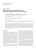
In Figure 5, an example of n
= 1000 gray code bits
selected with Gentleboost procedure is reported. Selected bits
are shown as black or white points on the different gray code
planes. This map indicates that a red-eye patch should have
1 in the position coloured in white and 0 in the positions
colored in black. Once gray code bits and the corresponding
weak classifiers parameters are learned, a new patch can be
classified by using the sign of (8).
The approach described above does not take into account
spatial relationship between selected gray code bits. Spatial
information is useful to make the classification task stronger
(e.g., pupil is surrounded of sclera). To overcome this
problem we coupled the gray codes bits selected at the
first learning stage using xor operator to obtain a new
set of n
2
binary features. We randomly select a subset
containing m of these features and performed a second round

of Gentleboost procedure to select the most discriminative
spatial relationship among the m randomly selected. This
new classifier is combined with the one learned previously
to perform final eye and non-eye patches classification.
Due to the multimodally nature of the patches involved
in our problem (i.e., colours, orientation, shape, etc.), a
single discriminative classifier could fail during classification
task. To get through this weakness, we propose to perform
first a clustering of the input space and then apply the two
stage boosting approach described above on each cluster.
More specifically, during the learning phase, the patches are
clustered by using K-means [16] in their original color space
producing the subsets of the input patches with the relative
prototypes; hence, the two stages of boosting described above
are performed on each cluster. During the classification stage,
a new patch is first assigned to a cluster according to the
closest prototype and then classified taking into account the
two additive models properly learned for the cluster under
consideration.
Experimental results reported in Section 4 confirm the
effectiveness of the proposed strategy.
3.3. Boosting for Binary Classification Exploiting Gray Codes.
Boosting provides a way to sequentially fit additive models of
the form in (8) optimizing the following cost function [18]:
J
= E

e
−yH(g)


(9)
where y
∈{−1, 1} is the class label associated to the feature
vector g. In this work, y
= 1 is associated to the eye class
whereas y
=−1 is the label associated to the non-eye class.
The cost function in the (9) can be thought as a differentiable
upper bound of the misclassification rate [19].
There are many ways to optimize this function. A simple
and numerical robust way to optimize this function is called
Gentleboost [18]. This version of boosting procedure out-
performs other boosting variants for computer vision tasks
(e.g., face detection) [21]. In Gentleboost, the optimization
6 EURASIP Journal on Image and Video Processing
Figure 5: Selected gray code bits.
of (9) is performed minimizing a weighted squared error at
each iteration [22]. Specifically at each iteration I, the strong
classifier H is updated as H(g):
= H(g)+h
best
(g)where
the weak classifier h
best
is selected in order to minimize the
second-order approximation of the cost function in (9)as
follows:
h
best
= argmin

h
d
J

H

g

+ h
d

g


argmin
h
d
E

e
−yH(g)

y − h
d

g

2

(10)

Defining as w
j
= e
−y
j
H(g
j
)
the weight for the training
sample j and replacing the expectation with an empirical
average over the training data, the optimization reduces in
minimizing the weighted squared error as follows:
J
wse
(
h
d
)
=
M

j=1
w
j

y
j
− h
d


g
j

2
(11)
where M is the number of samples in the training set.
The minimization of J
wse
depends on the specific form
of the weak classifiers h
d
. Taking into account the binary
representation of samples (i.e., the gray code of each patch),
in the present proposal we define the weak classifiers as
follows:
h
d

g

=
⎧
⎨
⎩
a
d
if g
d
= 1
b

d
if g
d
= 0
(12)
In each iteration the optimal a
d
and b
d
for each possible
h
d
can be obtained through weighted least squares as follows:
a
d
=

M
j
=1
w
j
y
j
δ

g
d
= 1



M
j=1
w
j
δ

g
d
= 1

b
d
=

M
j=1
w
j
y
j
δ

g
d
= 0


M
j

=1
w
j
δ

g
d
= 0

(13)
The best weak classifier h
best
is hence selected in each
iteration of the boosting procedure such that the cost of (11)
is the lowest as follows:
h
best
= argmin
h
d
J
wse
(
h
d
)
(14)
Finally, before a new iteration the boosting procedure
makes the following multiplicative update to the weights
corresponding to each training sample:

w
j
:= w
j
e
−y
j
h
best
(g
j
)
(15)
This update increases the weight of samples which are
misclassified (i.e., for which y
j
H(g
j
) < 0) and decreases the
weight of samples which are correctly classified.
The procedures employed for learning and classifica-
tion on the proposed representation are summarized in
Algorithm 1 and Algorithm 2. In the learning stage, we
initialize the weights corresponding to the elements of the
training set such that the number of the samples within each
classistakenintoaccount.Thisisdonetoovercomethe
problems that can occur due to the unbalanced number of
training samples within the considered classes.
3.4. Red-Eyes Correction. Once the red-eyes have been
detected, the correction step is performed. Usually the red-

eye artifact consists of a red pupil with a white glint. This
area is devoted to absorb light and thus should be dark.
To transform the red pupil to a dark region, a desaturation
and a brightness reduction is accomplished [1, 2]. The
region of connected red pixels is used to fix the area
that must be desaturated. To prevent unpleasant transition
from the iris to the pupil, red-eye artifact is replaced by
a mask with equal dimensions where each value is used
as weighted brightness/desaturation reduction factor. The
correction mask M isbasedona32
× 32 fixed point LUT
with Gaussian shape (Figure 6).Themaskisresizedthrough
a bilinear resampling to fit the dimension of the region of
connected red pixels under consideration.
EURASIP Journal on Image and Video Processing 7
Input:AsetofgraycodevectorsG ={g
1
, , g
M
}, and corresponding
labels Y
={y
1
, , y
M
}
Output: A strong classifier H(g) =

n
i

=1
h
i
(g)
begin
C
+
:={j | y
j
= 1};
C
−
:={j | y
j
=−1};
w
j∈C
+
:=
1
2|C
+
|
;
w
j∈C
−
:=
1
2|C

−
|
;
for i
= 1,2, , n do
for d
= 1,2, , D do
a
∗
d
:=

M
j
=1
w
j
y
j
δ(g
d
= 1)

M
j
=1
w
j
δ(g
d

= 1)
;
b
∗
d
:=

M
j
=1
w
j
y
j
δ(g
d
= 0)

M
j
=1
w
j
δ(g
d
= 0)
;
h
∗
d

(g):=

a
∗
d
if g
d
=1
b
∗
d
if g
d
=0
J
wse
(h
∗
d
):=

M
j
=1
w
j
(y
j
− h
∗

d
(g
j
))
2
;
p
i
:= argmin
d
J
wse
(h
∗
d
);
a
i
:= a
∗
p
i
;
b
i
:= b
∗
p
i
;

h
i
(g):=

a
i
if g
p
i
=1
b
i
if g
p
i
=0
w
j
:= w
j
e
−y
j
h
i
(g
j
)
;
H(g):

=

n
i
=1
h
i
(g)
end
Algorithm 1: Learning.
Input: The strong classifier H,andanewgraycodesampleg to be classified
Output: The inferred class y
∈{−1,1}
begin
y :
= sign(H(g));
end
Algorithm 2: Classification.
0
20
40
60
80
100
Figure 6: Brightness-saturation mask.
Let I
r
c
the channel c ∈{R,G, B}, of a region of interest r
within the image I. For each channel c

∈{R, G, B}, the pixels
(x, y) belonging to the region I
r
are corrected as follows:
I
r
c

x,y

=
⎧
⎪
⎪
⎪
⎨
⎪
⎪
⎪
⎩
I
r
c

x,y

I
r
R


x,y

, I
r
G

x,y

, I
r
B

x,y

∈W
I
r
G

x,y

M

x,y

otherwise
(16)
where W is a surrounding of the “white” color which can
slightly vary in terms of lightness, hue, and saturation. This
means that to prevent glint from disappearing only red

pixels are desatured (the whitish pixels are excluded from the
brightness processing).
8 EURASIP Journal on Image and Video Processing
Table 1: Estimated eye sizes taking into account the distance from the camera.
Distance from the sensor (m) 0.20 0.40 0.60 0.80 1.00 1.20 1.40 1.60 1.80 2.00 2.20 2.40 2.60 2.80 3.00
Pupil Diameter (pixels) 52 26 17 13 10 9776554443
Figure 7: Example of clusters prototypes obtained in an LOOCV run.
4. Experimental Settings and Results
The proposed red-eye removal pipeline has been tested
on a dataset of 390 images in which 1049 red eyes have
been manually labeled. The dataset has been collected
from various sources, including digital single-lens reflex
(DSLR) cameras, compact cameras, personal collections, and
internet photos. Single red eyes, as well as high variability
of red-eyes colors, poses, and shapes, have been considered
in building the dataset. In order to accurately assess the
proposed approach, the size of the eyes to be detected in
the collected images must be small enough to ensure that
also the smallest red eyes can be detected and corrected. The
basic requirement considered in our experimental phase is
that the red eyes must be accurately detected and corrected
up to three-meter distance from the camera. Tab le 1 presents
the estimated eye sizes, in pixels, for XGA image size (1024
×
768), with the assumption that the average eye is directed
to the camera. In this paper, the collected images have been
considered with an XGA image resolution, and the minimum
and maximum estimated pupil diameters (Ta bl e 1)have
been taken into account in building the dataset for testing
purposes.

For each image of the dataset, the pixels belonging to
red eyes artifacts have been manually labeled as red-eye
pixels. The parameters Min
h
,Max
h
, t
s
,Min
s
,Max
s
,Min
ρ
,
Max
ρ
,andMax
η
involved in the first stage of the proposed
approach (see Section 3.1) have been learned taking into
account the true and false red-eyes pixels within the labeled
dataset. To this aim, a full search procedure on a grid of
equispaced points in the eight- dimensional parameters’
space was employed. For each point of the grid, the correct
detection and false positives rates of the true red-eyes pixels
within the dataset were obtained. The tuple of parameters
with the best tradeoff between correct detection and the
false positives have been used to perform the final filtering
pipeline. A similar procedure was employed to determine the

subspace W of the RGB space involved in the correction step
to identify pixels belonging to the glint area.
In order to evaluate the classification performance of the
proposed method, the leave-one-out cross validation proce-
dure (LOOCV) has been employed. Each run of LOOCV has
involved a single image as test, and the remaining images as
training data. This is repeated to guarantee that each input
image is used once as test image. At each run of LOOCV, the
parameters of the filtering pipeline have been set to maximize
correct detection and minimize false positives. At each run of
LOOCV, the training images have been clustered, and then
the two-stage boosting approach described in Section 3.2 has
been performed on each cluster. Seven clusters (Figure 7)and
800 binary features for the additive classifiers corresponding
to the clusters have been used on each LOOCV run. The
maximum number of iterations used by boosting procedure
to obtain the 800 binary features was 1400. The final results
have been obtained averaging on the results of the overall
LOOCV runs.
Taking into account both, the filtering and the classifi-
cation stages, the hit rate of the proposed red-eyes detector
is 83.41%. This means that 875 red eyes have been correctly
detected with respect to the 1049 red eyes of the 390 input
images whereas only 34 false positives have been introduced.
In Figure 8, the training ability increasing the number of
bits is shown in terms of Hit Rates (Figure 8(a)) and False
Positives (Figure 8(b)).
In Figure 9, two examples of misclassified patches are
reported, in Figure 9(a), a “golden” eye is depicted (another
possible artifact due to similar acquisition problem). The

underlying structure in Figure 9(b) is probably the main
reason of misclassification.
In order to point out the usefulness of the proposed
cluster-based boosting, as well as the usefulness of the
spatial relationship introduced by using xor operation on
gray codes bits, we have repeated tests considering dif-
ferent configurations. Results reported in Ta bl e 2 confirm
the effectiveness of the rationale beyond the proposed
method.
To properly evaluate the overall red-eyes removal
pipeline, the qualitative criterion proposed in [14]was
adopted to compare the proposed solution with respect to
existing automatic solutions. According to [14], we divided
False Positive (FP) and False Negative (FN) to distinguish
different detection cases as follows:
FP
c
:criticalFP (e.g., visible FP on foreground, like
faces),
FP
n
: noncritical FP (e.g., undistinguishable FP on
foreground),
FN
m
: mandatory FN (e.g., red eyes well distinguish-
able),
FN
d
:desirableFN (e.g., small red eyes with low local

contrast).
EURASIP Journal on Image and Video Processing 9
72
74
76
78
80
82
84
(%)
200 400 600 800
(bit)
77.22%
76.84%
78.65%
83.41%
(a) Hit rates
0
10
20
30
40
50
60
70
80
200 400 600 800
(bit)
76
55

36
34
(b) False positives
Figure 8: Performances increasing number of bits.
(a) False negative (b) False positive
Figure 9: Examples of misclassified patches.
Table 2: Comparison of different configurations.
Configuration Hit Rate False Positives
Gray Codes 75.98% 47
Gray Codes + Clustering 77.51% 44
Gray Codes + XOR 79.31% 36
GrayCodes+Clustering+XOR 83.41% 34
The quality criterion proposed in [14] takes also into
account unwanted situation in which the automatic correc-
tion is performed on only one eye from pair. The number
of faces with one corrected eye from pair of red eyes
is indicated with N
p
. Regarding correction factors, two
cases are distinguished: corrected eyes that look worse of
original red eyes (C
i
) and situations when retouching is
noticeable, but it does not irritate strongly (C
n
). To obtain
a unique quality criterion (Q
c
), authors of [14] weighted the
aforementioned factors according to observers’ opinions as

follows:
Q
c
= 1 −
1
N
t
(
1.3
× FN
m
+0.7 × FN
d
)
−
1
N
t

3.6 × FP
c
+0.4 × FP
n
+1.6 × N
p

−
1
N
t

(
2.1
× C
i
+0.3 × C
n
)
(17)
where N
t
is the total number of red eyes within the test
dataset.
The proposed pipeline has been compared with respect
to the following automatic (mainly commercial) solutions:
Vo lk en et al . [ 13], NikonView V6.2.7, KodakEasyShare
V6.4.0, StopRedEye! V1.0, HP RedBot, Arcsoft PhotoPrinter
V5, and Cyberlink MediaShow. Experiments have been done
using effective commercial software and the implementation
of [13] provided by the authors. NikonView approach is
mainly based on [12].
As reported in Tab le 3 , the proposed approach has
obtained the best performances in terms of both, hit rate
and quality criterion. Moreover, the proposed approach
outperforms the method we have presented in [23]alsoin
terms of computational complexity. Despite the complete set
of images used in the experiments is not publicly available,
since most of the photos are taken from private collections,
some examples with corresponding results are available at the
following web address: />EurasipSpecialIssue2010.
4.1. Computational Complexity. To evaluate the complexity,

a deep analysis has been performed by running the proposed
pipeline on an ARM926EJ-S processor instruction set sim-
ulator. We have chosen this specific processor because it is
widely used in embedded mobile platforms. The CPU run
at 300 MHz and both data and instruction caches have been
fixed to 32 KB. The bus clock has been set to 150 MHz, and
the memory read/write access time is 9 ns. The algorithm has
been implemented using bitwise operators to work on colour
maps and fixed- point operations. Due to the dependence
of the operations to the number of red clusters found in
the image, we have analyzed a midcase, that is an image
containing around 40 potential red eye zones, but only 2 of
them are real eyes to be corrected.
Ta bl e 4 contains a report of the performances of the
main steps of the proposed pipeline, assuming to work
on an XGA version (scaled) of the image: the redness
detection (Color Map), the processing on the generated maps
(Morphological Operations), the candidate extraction, the
classification step, and finally the correction of the identified
10 EURASIP Journal on Image and Video Processing
Table 3: Quality score of different red-eyes removal approaches.
Method FN
m
FN
d
FP
c
FP
n
N

p
C
i
C
n
Q
c
Hit Rate
Cyberlink MediaShow 270 86 40 19 39 122 61 0.1423 66.06%
Volken et al. [13] 179 117 150 1540 83 17 79
−0.5851 71.78%
KodakEasyShare V6.4.0 194 99 5 20 5 104 100 0.4243 72.07%
HP RedBot 174 109 26 45 85 99 150 0.2345 73.02%
NikonView V6.2.7 143 116 6 29 88 124 129 0.2944 75.31%
StopRedEye! V1.0 124 125 8 12 83 81 91 0.4161 76.26%
Arcsoft PhotoPrinter V5 132 103 10 78 80 89 82 0.3800 77.60%
Battiato et al. [23] 122 85 2260 20 64 0.6346 80.26%
Proposed Pipeline 114 60 9 25 46 34 79 0.6174 83.41%
Table 4: Performances of the main steps of the proposed pipeline.
Color Map Morphological Operations Candidate Extraction Classification Correction
Instructions 19.845.568 22.990.051 9.418.650 4.446.349 1.698.946
Core cycles 28.753.276 30.489.180 16.407.293 5.668.496 2.390.279
D$ R Hits 4.722.760 2.903.178 2.504.092 945.959 205.188
D$ W Hits 97.636 261.213 428.924 135.634 94.727
D$ R Misses 75.495 6.293 5.666 3.450 244
D$ W Misses 2 193.891 3.290 24.069 1.133
SEQ 538.136 17.486.089 48.539 40.177 4.100
NON-SEQ 77.321 122.234 9.841 22.366 1.533
IDLE 16.282.401 7.325.256 10.345.379 3.203.188 1.372.407
Wait states 615.457 253.103 58.380 62.543 5.633

Total 17.513.316 16.208.789 10.462.139 3.328.274 1.383.673
Milliseconds 117 108 70 22 9
eyes. The performances information reported in Ta bl e 4 is
related to the following computational resources.
(i) Instructions: counts the executed ARM instructions.
(ii) Core cycles: core clock ticks needed to make the
Instructions.
(iii) Data (D$): Read/Write Hits and Misses, cache mem-
ory hits and misses.
(iv) Seq and Nonseq: sequential and nonsequential mem-
ory accesses.
(v) Idle: represents bus cycles when the instruction bus
and the data bus are idle, that is, when the processor
is running.
(vi) Busy: counts busy bus cycles, that is, when the data
are transferred from the memory into the cache.
(vii) Wait States: the number of bus cycles introduced
when waiting for accessing the RAM (is an indicator
of the impact of memory latencies).
(viii) Total: is the total number of cycles required by the
specific function, expressed in terms of bus cycles.
(ix) Milliseconds: time required by the specific function
expressed in milliseconds.
The overall time achieved on this midcase is 326 ms. The
table highlights the efficiency of the classifier because it is
mainly based on bit comparisons. Considering patches scaled
at 32
× 32 before the classification stage, the classifier is
essentially a comparison of 32
×32 bit words for each channel

with complexity in the range of one operation per pixel. For
this reason, it is very fast and light. Also the correction is very
light because, as explained in Section 3.4, it is based on the
resampling of a precomputed Gaussian function. The impact
on memory is valuable only on the map processing, where
data are processed several times, whereas in the remaining
steps of the pipeline the weight of the instructions determines
the main part of process timing.
We cannot compare the performances and complexity
of our methodology with other methods because the other
proposed methods are commercial ones; hence, the related
codes are not available for the analysis.
5. Conclusion and Future Works
In this paper, an advanced red-eyes removal pipeline has
been discussed. After an image filtering pipeline is devoted
to select only the potential regions in which red-eye artifacts
are likely to be, a cluster-based boosting on grey codes- based
features is employed for classification purpose. Red eyes are
then corrected through desaturation and brightness reduc-
tion. Experiments on a representative dataset confirm the
real effectiveness of the proposed strategy which also allows
to properly managing the multimodally nature of the input
EURASIP Journal on Image and Video Processing 11
space. The obtained results have pointed out a good trade-
off between overall hit rate and false positives. Moreover, the
proposed approach has shown good performance in terms of
quality measure. Future works will be devoted to include the
analysis of other eyes artifacts (e.g., “golden eyes”).
References
[1] F. Gasparini and R. Schettini, “Automatic red-eye removal for

digital photography,” in Single-Sensor Imaging: Methods and
Applications For Digital Cameras, R. Lukac, Ed., CRC Press,
Boca Raton, Fla, USA, 2008.
[2] G. Messina and T. Meccio, “Red eye removal,” in Image
Processing for Embedded De vices, S. Battiato, A. R. Bruna, G.
Messina, and G. Puglisi, Eds., Applied Digital Imaging Ebook
Series, Bentham Science, 2010.
[3] F. Gasparini and R. Schettini, “A review of redeye detection
and removal in digital images through patents,” Recent Patents
on Electrical Engineering, vol. 2, no. 1, pp. 45–53, 2009.
[4] A. Patti, K. Konstantinides, D. Tretter, and Q. Lin, “Automatic
digital redeye reduction,” in Proceedings of the International
Conference on Image Processing (ICIP ’98), pp. 55–59, October
1998.
[5] S. Battiato, M. Guarnera, T. Meccio, and G. Messina, “Red
eye detection through bag-of-keypoints classification,” in
Proceedings of the International Conference on Image Analysis
and Processing, vol. 5716 of Lecture Notes in Computer Science,
pp. 528–537, 2009.
[6] M. Gaubatz and R. Ulichney, “Automatic red-eye detection
and correction,” in Proceedings of the International Conference
on Image Processing (ICIP ’02), pp. I/804–I/807, September
2002.
[7] J. S. Schildkraut and R. T. Gray, “A fully automatic redeye
detection and correction algorithm,” in Proceedings of the
International Conference on Image Processing (ICIP ’02),pp.
I/801–I/803, September 2002.
[8] S. Ioffe, “Red eye detection with machine learning,” in
Proceedings of the International Conference on Image Processing
(ICIP ’03), pp. 871–874, September 2003.

[9] L. Zhang, Y. Sun, M. Li, and H. Zhang, “Automated red-
eye detection and correction in digital photographs,” in
Proceedings of the International Conference on Image Processing
(ICIP ’04), pp. 2363–2366, October 2004.
[10] H. Luo, J. Yen, and D. Tretter, “An efficient automatic redeye
detection and correction algorithm,” in Proceedings of the 17th
International Conference on Pattern Recognition (ICPR ’04),pp.
883–886, August 2004.
[11] G. Petschnigg, R. Szeliski, M. Agrawala, M. Cohen, H. Hoppe,
and K. Toyama, “Digital photography with flash and no-flash
image pairs,” ACM Transactions on Graphics,vol.23,no.3,pp.
664–672, 2004.
[12] P. Corcoran, P. Bigioi, E. Steinberg, and A. Pososin, “Auto-
mated in-camera detection of flash eye-defects,” in Proceedings
of the International Conference on Consumer Electronics (ICCE
’05), pp. 129–130, January 2005.
[13] F. Volken, J. Terrier, and P. Vandewalle, “Automatic red-
eye removal based on sclera and skin tone detection,” in
Proceedings of the European Conference on Color in Graphics,
Imaging and Vision, 2006.
[14] I. V. Safonov, M. N. Rychagov, K. Kang, and S. H. Kim,
“Automatic red eye correction and its quality metric,” in Color
Imaging XIII: Processing, Hardcopy, and Applications, vol. 6807
of Proceedings of SPIE, San Jose, Calif, USA, 2008.
[15] A. M. Ferman, “Automatic detection of red-eye artifacts in
digital color photos,” in Proceedings of the IEEE International
Conference on Image Processing (ICIP ’08), pp. 617–620,
October 2008.
[16] R.O.Duda,P.E.Hart,andD.G.Stork,Pattern Classification,
Wiley-Interscience, New York, NY, USA, 2nd edition, 2000.

[17] R. C. Gonzalez and R. E. Woods, Digital Image Processing,
Prentice-Hall, Englewood Cliff
s, NJ, USA, 2006.
[18] J. Friedman, T. Hastie, and R. Tibshirani, “Additive logistic
regression: a statistical view of boosting,” Annals of Statistics,
vol. 28, no. 2, pp. 337–407, 2000.
[19] R. E. Schapire, “The boosting approach to machine learning:
an overview,” in Proceedings of the MSRI Workshop on
Nonlinear Estimation and Classification, 2001.
[20] R. E. Schapire, “The strength of weak learnability,” Machine
Learning, vol. 5, no. 2, pp. 197–227, 1990.
[21] R. Lienhart, A. Kuranov, and V. Pisarevsky, “Empirical analysis
of detection cascades of boosted classifiers for rapid object
detection,” in Proceedings of the 25th Symposium of the German
Association for Pattern Recognition (DAGM ’03), vol. 2781, pp.
297–304, Magdeburg, Germany, September 2003.
[22] A. Torralba, K. P. Murphy, and W. T. Freeman, “Sharing visual
features for multiclass and multiview object detection,” IEEE
Transactions on Pattern Analysis and Machine Intelligence, vol.
29, no. 5, pp. 854–869, 2007.
[23] S. Battiato, G. M. Farinella, M. Guarnera, G. Messina, and
D. Rav
`
ı, “Red-eyes removal through cluster based linear
discriminat analysis,” in Proceedings of the IEEE International
Conference on Image Processing (ICIP ’10), pp. 2185–2188,
September 2010.