Báo cáo hóa học: " Research Article An MCMC Algorithm for Target Estimation in Real-Time DNA Microarrays Haris Vikalo and Mahsuni Gokdemir" ppt

Hindawi Publishing Corporation
EURASIP Journal on Advances in Signal Processing
Volume 2010, Article ID 736301, 8 pages
doi:10.1155/2010/736301
Research Article
An MCMC Algorithm for Target Estimation in
Real-Time DNA Microarrays
Haris Vikalo and Mahsuni Gokdemir
Department of Electrical and Computer Enginee ring, The University of Texas, Austin, TX 78712-0240, USA
Correspondence should be addressed to Haris Vikalo,
Received 1 February 2010; Accepted 15 July 2010
Academic Editor: Harri L
¨
ahdesm
¨
aki
Copyright © 2010 H. Vikalo and M. Gokdemir. This is an open access article distributed under the Creative Commons Attribution
License, which permits unrestricted use, distribution, and reproduction in any medium, provided the original work is properly
cited.
DNA microarrays detect the presence and quantify the amounts of nucleic acid molecules of interest. They rely on a chemical
attraction between the target molecules and their Watson-Crick complements, which serve as biological sensing elements (probes).
The attraction between these biomolecules leads to binding, in which probes capture target analytes. Recently developed real-
time DNA microarrays are capable of observing kinetics of the binding process. They collect noisy measurements of the amount
of captured molecules at discrete points in time. Molecular binding is a random process which, in this paper, is modeled by a
stochastic differential equation. The target analyte quantification is posed as a parameter estimation problem, and solved using a
Markov Chain Monte Carlo technique. In simulation studies where we test the robustness with respect to the measurement noise,
the proposed technique significantly outperforms previously proposed methods. Moreover, the proposed approach is tested and
verified on experimental data.
1. Introduction
Molecular biosensors [1] are devices that contain a biological
sensing element closely coupled with a transducer. They

measure interaction of biomolecules of interest (target ana-
lytes) with the biological sensing element, and generate signal
proportional to the amount of the analyte molecules. Detec-
tion in affinity biosensors [2] relies on chemical attraction
between target analytes and their molecular complements,
which serve as biological sensing elements (probes). The
attraction between these biomolecules (their affinity for
each other) leads to binding, in which probes capture
target analytes. For instance, nucleic acid probes (DNA,
RNA, or synthetic oligonucleotides) capture their Watson-
Crick complements, antibody probes capture antigens, cell
receptor probes capture ligands, and so forth. A transducer
then converts the number of complex molecular structures
that are formed due to the binding into a signal. Affinity
biosensors can be multiplexed, which led to the development
of microarrays—arrays of affinity biosensors capable of
testing a large number of analytes simultaneously. DNA
microarrays [3], in particular, are capable of screening tens
or even hundreds of thousands of different gene sequences
at the same time, revealing critical information about the
functionality of cells, effects of drugs on organisms, and
so forth. Microarrays are time- and cost-efficient, and may
enable exciting new applications in drug discovery, medicine,
defense systems, and environmental monitoring.
Despite their enormous potential, however, microarrays
have not fully met the expectations of the research com-
munity and industry. Although in principle reliable [4],
their performance still leaves something to be desired [5, 6].
Today, the sensitivity, dynamic range, and resolution of DNA
microarrays are limited by interference, noise, probe satu-

ration, and other sources of errors in the analyte detection
procedure. Several of these limitations stem from the fact that
the molecular binding is a stochastic process, which many of
the conventional affinity biosensors attempt to characterize
based on a single measurement of its equilibrium, that is,
by taking one sample from the steady-state distribution of
the binding process. On the other hand, real-time DNA
microarrays are capable of taking multiple temporal samples
2 EURASIP Journal on Advances in Signal Processing
of a binding process [7–9]. However, analyte estimation
therein is typically performed using only the data collected
in the equilibrium, and rarely relies on the kinetics [10].
In [11], analyte targets in real-time DNA microarrays
are estimated using the temporally sampled kinetics of
the binding process. However, the kinetics process there is
described using a deterministic model. In this paper, we
propose a comprehensive stochastic model of the binding
process and state a Markov Chain Monte Carlo (MCMC)
algorithm for the estimation of the target analytes. The
performance of the proposed algorithm is tested on both
synthetic and experimental data.
The paper is organized as follows. In Section 2,we
describe the stochastic differential equation modeling the
probe-target binding process. In Section 3, parameter esti-
mation in discretely sampled diffusionprocessesisdescribed,
assuming noiseless data acquisition. An MCMC algorithm
for the parameter estimation in the realistic noisy scenario
is discussed in Section 4. Section 5 shows simulation results,
while the experimental verification is provided in Section 6.
Section 7 concludes the paper and outlines future work.

2. Stochastic Model
Let n
t
denote the total number of analyte molecules, and let
n
c
(t) denote the number of those that are bound to their
corresponding probes at time t. For simplicity, let us assume
that the number of probe molecules, n
p
, is greater than n
t
.
Then the probability that a free analyte molecule becomes
captured during the (t, t + Δt) time interval is
p
b
= k
1

1 −
n
c
(
t
)
n
p

Δt,(1)

where k
1
denotes the association rate of the capturing process
assuming an unlimited amount of probe molecules, and
(1
− n
c
(t)/n
p
) is the fraction of the probe molecules that
are available. Assuming that the binding events are mutually
independent and that n
t
is large, the number of analyte
molecules captured during the (t, t+Δt) time interval follows
Binomial distribution with mean (n
t
−n
c
(t))p
b
and variance
(n
t
− n
c
(t))p
b
(1 − p
b

). For large n
t
(which in the biosensor
context is certainly the case), this Binomial distribution can
be approximated by a Gaussian
N

(
n
t
−n
c
(
t
))
p
b
,
(
n
t
−n
c
(
t
))
p
b

1 − p

b

. (2)
Following a similar argument, it can be shown that the
number of analyte molecules which are released during the
(t, t + Δt) time interval is distributed with
N

n
c
(
t
)
p
r
, n
c
(
t
)
p
r

1 − p
r

,(3)
where p
r
= k

−1
Δt is the probability of release of a captured
analyte molecule, and where k
−1
denotes the disassociation
rate (for more details see, e.g., [12]).
Now, n
c
(t) is a continuous-time Markov process. Its
states are discrete, but under some mild conditions [13] (the
transition probabilities do not change abruptly and n
c
(t)is
sufficiently large, both of which are readily satisfied in the
biosensor context), we can describe the dynamics of n
c
(t)by
the following stochastic differential equation (SDE)
n
c
(
t + dt
)
−n
c
(
t
)
= μ
(

n
c
, θ, t
)
dt + σ
(
n
c
, θ, t
)
dW,(4)
where θ
= [n
t
n
p
k
1
k
−1
], the drift μ(n
c
, θ, t) and diffusion
σ(n
c
, θ, t)coefficients are given by
μ
(
n
c

, θ, t
)
= k
1
n
p
−n
c
n
p
(
n
t
−n
c
)
−k
−1
n
c
,
σ
(
n
c
, θ, t
)
=

k

1
n
p
−n
c
n
p
(
n
t
−n
c
)
+ k
−1
n
c

1/2
,
(5)
and where W denotes the Wiener process (detailed deriva-
tion is in [12]).
Real-time DNA microarrays collect noisy observations
of the temporally sampled diffusion process (4). Ultimately,
we would like to use the collected observations to estimate
parameters of the model θ (including n
t
, the number of
target molecules). A survey of techniques for parameter

estimation of discretely observed diffusion processes is given
in [14]. These techniques include (i) estimating functions
[15]; (ii) indirect inference and efficient method of moments
[16]; (iii) Bayesian analysis and Markov Chain Monte Carlo
(MCMC) methods [17–20]; (iv) analytical and numerical
approximation of the likelihood function [21–23]. For
Bayesian analysis and the MCMC methods, the SDE is first
discretized in-sync with the measurements, using time incre-
ments equal to the sampling period of the measurements.
Additional time points are introduced between the samples
[24], and the corresponding values of n
c
(t)aretreatedas
missing data points. The MCMC techniques [25] are then
used to generate the missing data points. We should point
out that MCMC techniques may be employed to estimate
parameters in fairly general SDE models where the drift and
diffusion coefficients are allowed to be nonlinear functions of
diffusion process, or where parameters may enter into these
coefficients nonlinearly. This is the case for the SDE model of
real-time biosensor arrays (4).
In this paper, we rely on MCMC techniques to estimate
the parameters θ of the SDE model (4) observed at discrete
points in time and subject to measurement noise. In order to
derive suitable proposal densities in the MCMC algorithm,
we assume that the drift and diffusion coefficients satisfy the
Lipschitz and linear growth conditions




μ
(
x, θ, t
)
−μ

y, θ, t



+


σ
(
x, θ, t
)
−σ

y, θ, t



≤
C


x−y



,
(6)


μ
(
x, θ, t
)


2
+ |σ
(
x, θ, t
)
|
2
≤ C
2

1+|x|
2

(7)
for some positive constant C (see, e.g., [26]). For the sake of
clarity of presentation, in the next section we first consider
the noise-free case. Then, in the following section, we turn
our attention to the noisy case.
3. Parameter Estimation in the Noise-Free Case
Denote the set of N observations acquired over [0, T]by

O
= {n
c
(t
1
), n
c
(t
2
), , n
c
(t
i
), , n
c
(t
N
)},wheret
i
= iΔt
EURASIP Journal on Advances in Signal Processing 3
where Δt denotes the sampling (data acquisition) period. In
principle, we may try to use the observed data to form the
log-likelihood,
L
(
θ
| n
c
(

t
1
)
, , n
c
(
t
N
))
=
N

i=1
L
i
(
θ
)
,(8)
where L
i
(θ) = log{p(n
c
(t
i
), n
c
(t
i+1
); θ)}, and then find


θ by maximizing L(θ, ·). The challenge, however, is that
p(n
c
(t
i
), n
c
(t
i+1
); θ), a closed form expression for the transi-
tional density between two consecutive discrete observation
points is unavailable for the system in (4). Therefore,
the likelihood function is often approximated via various
numerical techniques [27, 28]. Here we describe the data
augmentation procedure.
Consider the SDE (4) over a time interval [0, T], and
assume that we uniformly sample n
c
(t)everyΔt = T/N.
Therefore, we assume that the value n
c
(t
i−1
) at the beginning
of the time interval (t
i−1
, t
i
) is known. For convenience,

denote x
i
= n
c
(t
i
). Finding exact analytical expression
for the transition density p(x
i
|x
i−1
, θ)appearsdifficult to
obtain. However, if Δt is very small, we could approximate
it by p(x
i
|x
i−1
, θ) ∼ N (μ
i
, σ
2
i
), where N (μ
i
, σ
2
i
) denotes the
normal distribution with mean μ
i

and variance σ
2
i
,andwhere
μ
i
= x
i−1
+ μ
(
x
i−1
, θ, t
i−1
)
Δt,
σ
2
i
= σ
2
(
x
i−1
, θ, t
i−1
)
Δt.
(9)
On the other hand, the sampling time Δt used for data

acquisition is typically not sufficiently small to justify the
approximation above. Therefore, we further discretize the
interval (t
i−1
, t
i
) dividing it into M subintervals, where each
subinterval is of the length Δτ
= Δt/M. Following [29], we
employ the Euler-Maruyama integration scheme to generate
points from a sample path of n
c
(t)on(t
i
, t
i
+(M − 1)Δτ).
[Note that t
i+1
= t
i
+ MΔτ.] Denote these points by z
j
,
j
= 0, 1, , M − 1, where z
0
= x
i
. We put all these latent

values between (t
i−1
, t
i
) into z = (z
1
, z
2
, , z
M−1
). The Euler-
Maruyama scheme generates z
j
by recursively computing
z
j
= z
j−1
+ μ

z
j−1
, θ, t
i
+

j − 1

Δτ


Δτ
+ σ

z
j−1
, θ, t
i
+

j − 1

Δτ

ΔW
j
,
(10)
j
= 1,2, , M −1, where ΔW
j
= W(t
i
+ jτ) − W(t
i
+(j −
1)τ) ∼ N (0,Δτ), and where W(0) = 0.
Now, we can form the joint distribution of latent values
z with x
i
given x

i−1
and θ and then integrate out the missing
values to find the transition density.
p
(
x
i
| x
i−1
, θ
)
=

p
(
x
i
, z | x
i−1
, θ
)
dz
=

M

m=1
p
(
z

m
| z
m−1
, θ
)
dz
(11)
where x
i
= z
M
and x
i−1
= z
0
and we use the Markov property
of diffusion process. However, this multidimensional integral
is not easy to evaluate. As a standard approach, we can
use Monte Carlo integration together with the importance
sampler to approximate this integral:
p
(
x
i
| x
i−1
, θ
)
=


p
(
x
i
, z | x
i−1
, θ
)
q
(
z
)
q
(
z
)
dz,

p
(
x
i
| x
i−1
, θ
)
=
1
K
K


k=1

M
m
=1
p
(
z
m
| z
m−1
, θ
)

M−1
m=1
q
(
z
m
| z
m−1
, θ
)
,
(12)
In this equations, we are using the fact that n
c
(t)isa

Markov process to write the joint distribution as a product
of marginal distributions. We are generating K sample paths
of the n
c
(t) on the time interval (t
i−1
, t
i
) to approximate
the transition density. Now, we must construct efficient
importance samplers to draw the missing samples z
j
.
The importance sampler that we consider draws z
j
from
the Euler approximation of the SDE ([24]). Then, since the
p(z
m
|z
m−1
, θ) is also approximated using this discrete model;
the first M
− 1 terms of the target density p(z
m
|z
m−1
, θ)
and the density of the importance sampler q(z
m

|z
m−1
, θ)
are identical and cancel each other and the only remaining
term is the p(x
i
|z
M−1
, θ). After this cancelation, we have the
following approximate transition density:

p
(
x
i
| x
i−1
, θ
)
=
1
K
K

k=1
p
(
x
i
| z

M−1
, θ
)
. (13)
Therefore, the last point obtained by the scheme (10)
is z
M−1
, which can be regarded as a sample of the process
n
c
(t)att
i−1
+(M − 1)Δτ. The Euler-Maruyama inte-
gration procedure is repeated K times, generating points
z
1
M
−1
, z
2
M
−1
, , z
K
M
−1
. The approximation converges weakly
to the desired process as M increases (see, e.g., [28]and
the references therein). Thus the transition density can be
approximated by

p
(
x
i
| x
i−1
, θ
)
≈

p
(
x
i
| x
i−1
, θ
)
∼
1
K
K

k=1
N

μ
k
i
,


σ
k
i

2

, (14)
where
μ
k
i
= z
k
M
−1
+ μ

z
k
M
−1
, t
i−1
+
(
M −1
)
Δτ, θ


Δτ,

σ
k
i

2
= σ
2

z
k
M
−1
, t
i−1
+
(
M −1
)
Δτ, θ

Δτ,
(15)
for each k
= 1, 2, , K
To summarize, in each time interval (t
i−1
, t
i

)weperform
the following steps.
(1) Starting from z
0
= x
i−1
= n
c
(t
i−1
), employ the Euler-
Maruyama technique (10) to generate K samples of
the process n
c
(t)att = t
i−1
+(M − 1)Δτ. These
samples are denoted by z
k
i
,1≤ k ≤ K.
(2) Use z
1
M
−1
, z
2
M
−1
, , z

K
M
−1
to estimate the transition
density according to (14).
The approximate transition density converges to the true
one as K
→∞. We repeat the above procedure to obtain
4 EURASIP Journal on Advances in Signal Processing
approximate transition densities

p(x
i
|x
i−1
, θ)foreachi =
1, 2, , N, and form the likelihood function

L
(
θ
)
=
N

i=1
log

p
(

x
i
| x
i−1
, θ
)
. (16)
Finally,

L(θ) is maximized over θ. For large M, K, the
resulting

θ approaches the true ML estimate of θ.
To lower the computational complexity of the approach
described in this section, various modifications have been
proposed. For instance, alternative importance samplers are
employed to accelerate the convergence of the Monte Carlo
integration, resulting in significant computational savings
(see, e.g., [30] and the references therein). We shall not
pursue these alternative importance samplers here. Instead,
we switch our attention to the estimation problem in the
noisy measurement case.
4. An MCMC Algorithm for Parameter
Estimation in Noisy Case
The technique described in the previous section assumes
noise-free data. In this section, we focus our attention on the
more realistic noisy scenario. We do not explicitly form the
likelihood function but instead rely on an MCMC technique
which alternates between drawing missing data conditioned
on parameters and observations, and the parameters con-

ditioned on the missing data and the observations. Assume
that the continuous diffusion (4) is sampled, and denote
the obtained noisy observations by y
iM
, that is, assume the
continuous-discrete model
dn
c
= μ
(
n
c
, θ, t
)
dt +

β
(
n
c
, θ, t
)
dW,
y
iM
= n
c
(
t
i

)
+ v
i
= n
c
(
iMΔτ
)
+ v
i
,
(17)
where v
i
denotes iid Gaussian noise N (0,
2
), and where
β(n
c
, θ, t) = σ
2
(n
c
, θ, t) is introduced for notational con-
venience. (Note that for the sake of simplicity we set the
transduction coefficient in the measurement equation to 1.)
Let O denote the set of collected noisy observations, O
=
{
y

0
, y
M
, , y
iM
, , y
K
},whereK = NM. Furthermore, we
denote z
i
= n
c
(iΔτ) and collect the points z
i
into Z =
{
z
0
, z
1
, , z
M
, , z
2M
, , z
K
}. (Note that y
iM
is a noisy
observation of z

iM
.)
Following [19], to enable estimation of the parameters
θ, we form the joint posterior density of the parameters and
simulated missing data
p
(
Z, θ
| O
)
∝ p
(
θ
)
p
(
z
0
)
K−1

i=0
p
(
z
i+1
| z
i
, θ
)

N

i=0
p

y
iM
| z
iM
, θ

,
(18)
where the transition density p(z
i+1
|z
i
, θ) and the measure-
ment density p(y
i
|z
i
, θ)aregivenby
p
(
z
i+1
| z
i
, θ

)
= N

z
i+1
; z
i
+ μ
i
Δτ, β
i
Δτ

,
p

y
i
| z
i
, θ

= N

y
i
; z
i
, 
2


(19)
and where μ
i
= μ(z
i
, θ, iΔτ), β
i
= β(z
i
, θ, iΔτ). We rely
on the Gibbs sampling technique to draw the missing data
conditioned on the current state of the parameters and
observations, and draw the parameters conditioned on the
simulated missing data and observations. This procedure
generates a Markov chain whose stationary distribution is
(18). Expressed algorithmically, we perform the following
steps.
(1) Initialize parameters and latent values. Use linear
interpolation between the measured points in O to
initialize Z. Set the iteration counter to s
= 1.
(2) In the iteration s,drawZ
s
∼ p(·|θ
s−1
, O).
(3) Draw θ
s
∼ p(·|Z

s
, O) via Gaussian random walk
update.
(4) Set s
= s +1andgotostep2.
Finding the analytical expressions of the distributions
in steps 2 and 3 appears infeasible. Hence, we employ
the Metropolis-Hasting (M-H) algorithm to compute them
numerically. In step 2, we generate a single component of Z
(i.e., z
i
) at a time (the so-called single site update), where
there are four different cases depending on the value of the
time index i.Case1 deals with drawing the missing data z
i
for which there are no corresponding noisy observations in
O (i.e., i is not an integer multiple of M). On the other hand,
Cases 2–4 deal with drawing the missing data z
i
for which
we do acquire noisy measurements. Among these, Cases 3
and 4 deal with the missing data at the start and at the end
of the binding process, respectively (i.e., the boundary points
corresponding to i
= 0andi = K). Case 2 deals with drawing
the remaining missing data z
i
(i.e., i is an integer multiple of
M, i
/

=0, K).
Case 1. i (is not an integer multiple of M). In this case, the
conditional distribution is given by
p
(
z
i
| z
i−1
, z
i+1
, θ
)
∝ p
(
z
i
| z
i−1
, θ
)
p
(
z
i+1
| z
i
, θ
)
. (20)

Direct sampling from this distribution is not feasible.
Therefore, we need to employ the M-H algorithm.
Following [17], when the drift and the diffusion coeffi-
cients are constant it holds that
p
(
z
i
| z
i−1
, z
i+1
, θ
)
∼ N

1
2
(
z
i−1
+ z
i+1
)
,
1
2
βΔτ

. (21)

However, we need to consider a more general case where drift
and diffusion coefficients are functions of parameters θ and
the diffusion process z (clearly, this is the case for our model).
Now, drift and diffusion coefficients have bounded
growth as stated in (7); moreover, sample paths of the
diffusion process (i.e., the molecular binding process) are
continuous since the sample paths of the underlying Brow-
nian motion are continuous. This implies that the drift and
diffusion coefficients are locally constant. Thus, for small
time interval Δτ the previous result stated for constant drift
and diffusion coefficients also holds for arbitrary drift and
EURASIP Journal on Advances in Signal Processing 5
diffusion. The rigorous proof is given in [17]. It follows that
a suitable proposal density q(z
∗
i
|z
i−1
, z
i+1
, θ)isgivenby
N

z
∗
i
;
1
2
(

z
i−1
+ z
i+1
)
,
1
2
β
(
z
i−1
, θ
)
Δτ

. (22)
It can be shown that
q

z
∗
i
| z
i−1
, z
i+1
, θ

−→

p
(
z
i
| z
i−1
, z
i+1
, θ
)
, (23)
as Δt
→ 0. The proposed data point
z
∗
i
∼ N

1
2
(
z
i−1
+ z
i+1
)
,
1
2
β

(
z
i−1
, θ
)
Δτ

(24)
is accepted with probability min(1, α), where
α
=
p

z
∗
i
| z
i−1
, θ

p

z
i+1
| z
∗
i
, θ

p

(
z
i
| z
i−1
, θ
)
p
(
z
i+1
| z
i
, θ
)
×
q
(
z
i
| z
i−1
, z
i+1
, θ
)
q

z
∗

i
| z
i−1
, z
i+1
, θ

.
(25)
Here, z
i−1
is the value at the iteration s and z
i+1
is the value
obtained at iteration s
−1 of the Gibbs Sampler.
Case 2 (i is an integer multiple of M, i
/
=0, K). In this case,
the conditional distribution is
p

z
i
| z
i−1
, z
i+1
, y
i

, θ

∝
p
(
z
i
| z
i−1
, θ
)
p
(
z
i+1
| z
i
, θ
)
p

y
i
| z
i
, θ

.
(26)
Starting from (22), we can form the joint density of z

i
and y
i
conditioned on z
i−1
, z
i+1
and as
N

1
2

z
i−1
+ z
i+1
z
i−1
+ z
i+1

,
1
2

β
i−1
Δτβ
i−1

Δτ
β
i−1
Δτβ
i−1
Δτ +2
2

. (27)
From this joint Gaussian density, it is straightforward to
obtain the conditional one
q

z
∗
i
| z
i−1
, z
i+1
, y
i
, θ

∼
N

z
∗
i

; ψ, γ

, (28)
where the mean and the variance are given by
ψ
=
(
z
i−1
+ z
i+1
)
2
+
Δτβ
i−1

y
i
−
(
1/2
)(
z
i−1
+ z
i+1
)



β
i−1
Δτ +2
2

,
γ
=
β
i−1
Δτ
2
−
1
2
Δτβ
i−1

1
2
β
i−1
Δτ + 
2

−1
β
i−1
1
2

Δτ.
(29)
The proposed value z
∗
i
is accepted with probability min(1, α),
where
α
=
p

y
i
| z
∗
i
, θ

p

z
∗
i
| z
i−1
, θ

p

z

i+1
| z
∗
i
, θ

p

y
i
| z
i
, θ

p
(
z
i
| z
i−1
, θ
)
p
(
z
i+1
| z
i
, θ
)

×
q

z
i
| z
i−1
, z
i+1
, y
i
, θ

q

z
∗
i
| z
i−1
, z
i+1
, y
i
, θ

.
(30)
Case 3 (i
= 0). The conditional distribution is given by

p

z
0
| z
1
, y
0
, θ

∝ p
(
z
0
)
p
(
z
1
| z
0
, θ
)
p

y
0
| z
0
, θ


. (31)
Using the Euler approximation, we can write:
z
0
= z
1
−μ
0
Δτ + β
1/2
0
ΔW. (32)
Since sample paths of the diffusion process are continuous,
and since drift and diffusion coefficients have bounded
growth by assumption given in (7), μ and β are locally
constant. Hence, we can approximate μ
0
by μ
1
and β
0
by β
1
which leads to
z
0
≈ z
1
−μ

1
Δτ + β
1/2
1
ΔW. (33)
Then,
p
(
z
0
| z
1
, θ
)
∼ N

z
0
; z
1
−μ
1
Δτ, β
1
Δτ

. (34)
Combining this density with the measurement error density
given by
p


y
0
| z
0
, θ

=
N

y
0
; x
0
, 
2

, (35)
we obtain the joint density of y
0
and z
0
conditioned on z
1
and θ as

z
0
y
0


∼
N

z
1
−μ
1
Δτ
z
1
−μ
1
Δτ

,

β
1
Δτβ
1
Δτ
β
1
Δτβ
1
Δτ + 
2

. (36)

By applying the relation between the joint Gaussian distri-
bution and its corresponding conditionals, we arrive to a
suitable proposal density for the M-H algorithm given by
q

z
∗
0
| z
1
, y
0
, θ

∼ N

z
∗
0
; ψ, γ

, (37)
where the mean and the variance are defined as
ψ = z
1
−μ
1
Δτ +
Δτβ
1


y
0
−

z
1
−μ
1
Δτ


β
1
Δτ + 
2

,
γ
= β
1
Δτ − Δτβ
1

β
1
Δτ + 
2

−1

β
1
Δτ.
(38)
The proposed value z
∗
0
is chosen with probability min(1, α),
where
α
=
p

z
∗
0

p

y
0
| z
∗
0
, θ

p

z
1

| z
∗
0
, θ

p
(
z
0
)
p

y
0
| z
0
, θ

p
(
z
1
| z
0
, θ
)
×
q

z

0
| z
1
, y
0
, θ

q

z
∗
0
| z
1
, y
0
, θ

.
(39)
Case 4 (i
= K). Now the conditional distribution is
p

z
K
| z
K−1
, y
K

, θ

∝
p
(
z
K
| z
K−1
, θ
)
p

y
K
| z
K
, θ

(40)
By using the Euler transition density p(z
k
|z
k
− 1,θ) and the
measurement error density p(y
k
|z
k
, θ), we can form the joint

density of z
k
and y
k
conditioned on z
k−1
and θ as

z
K
y
K

∼
N

μ
μ

,

β
K−1
Δτβ
K−1
Δτ
β
K−1
Δτβ
K−1

Δτ + 
2

, (41)
where μ
= z
K−1
−μ
K−1
Δτ. It follows that
p

z
K
| z
K−1
, y
K
, θ

∼ N

z
K
; ψ, γ

, (42)
6 EURASIP Journal on Advances in Signal Processing
where the mean and the variance are given by
ψ

= z
K−1
+ μ
K−1
Δτ +
Δτβ
K−1

y
K
−

z
K−1
+ μ
K−1
Δτ


β
K−1
Δτ + 
2

,
γ
= β
K−1
Δτ − Δτβ
K−1


β
K−1
Δτ + 
2

−1
β
K−1
Δτ.
(43)
In this case, we can directly sample from the above density,
so there is no need for the M-H algorithm.
On another note, in step 3 of the Gibbs sampling
algorithm we update θ as θ
∗
s
= θ
s
+ Ω,whereΩ ∼ N (0, Γ)
and Γ
= diag(γ
i
). (These variances determine the mixing
properties of the generated Markov chain.) We again use the
M-H algorithm and accept θ
∗
s
with probability min(1, α),
where

α
=
L

θ
∗
| Z, O

L
(
θ | Z,O
)
=


K−1
i=1
p

z
i+1
| z
i
, θ
∗



N
i=0

p

y
iM
| z
iM
, θ
∗




K−1
i=1
p
(
z
i+1
| z
i
, θ
)


N
i=0
p

y
iM

| z
iM
, θ


.
(44)
When the noise variance is known, p(y
|z, θ) is independent
of the parameters θ and thus we can simplify α to
α
=


K−1
i=1
p

z
i+1
| z
i
, θ
∗




K−1
i=1

p
(
z
i+1
| z
i
, θ
)

. (45)
5. Simulation Results
We simulate the reaction (4), where the parameters are set to
n
p
= 10
5
, n
t
= 10
3
, k
1
= 10
−3
,andk
−1
= 10
−3
. The signal
is sampled (N

= 300), where the samples are perturbed
by an additive Gaussian noise (zero-mean, variance ε
2
). In
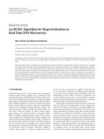
Figure 1, we compare the square root of the relative mean-
square error,

E{(n
t
− n
t
)
2
/n
2
t
}, of the MCMC algorithm
for stochastically modeled real-time microarrays and the
least-mean-squares estimation approach for deterministi-
cally modeled (by means of ordinary differential equations)
real-time microarrays (see [11] for details). (We assume that
all parameters other than n
t
are known.) The error is plotted
as a function of the observation noise variance (the error is
averaged over 100 trials). The simulation results indicate that
the proposed approach significantly outperforms the least-
mean-squares method over the broad range of parameters.
The Gibbs Sampler is performed with M
= 5andK =

1500. The burn-in period of the algorithm is 500 iterations,
while no more than 300-400 iterations are needed for the
convergence (see Figure 2).
6. Experimental Verification
To verify the proposed approach in experiments, we used
the real-time microarray data reported in [11]. In those
experiments, cDNA targets were generated from The RNA
Spikes, a commercially available set of 8 purified Esche richia
0 200 400 600 800 1000
0
0.02
0.04
0.06
0.08
0.1
0.12
0.14
0.16
0.18
√
RMSE
Noise variance
MCMC-stochastic model
LMS-deterministic model
Figure 1: The square root of the relative mean-square error,

E{(n
t
− n
t

)
2
/n
2
t
}, of the Gibbs Sampler and the least-mean-
squares estimation approach, as a function of the observation noise
variance of 100, 250, 500 and 1000.
0 100 200 300 400 500 600 700 800 900
0
1000
2000
3000
4000
5000
6000
7000
8000
9000
Number of target analytes
Number of iterations of Gibbs sampler
1000
Figure 2: The convergence of n
t
as a function of the number of
iterations.
Coli RNA transcripts purchased from Ambion Inc. Lengths
of the RNA sequences in the set are (750, 752, 1000, 1000,
1034, 1250, 1475, 2000), respectively. The RNA sequences
were reverse transcribed to obtain the cDNA targets, which

were then labeled with Cy5 dyes. Eight probes (25 mer
oligonucleotides) were designed and printed on slides, where
each probe was repeated in 6 different spots; hence, the
printed slides had 48 spots. We focus on two experiments,
one where the concentrations of the targets was 80ng/50 μL,
and the other where the concentrations of the targets was
16 ng/50 μl.
In order to mitigate the numerical problems caused
by large numbers (e.g., n
p
is on the order of 10
11
in the
experimental data), we scale down the variables in the SDE
(in particular, scaling factor k
= 10
6
was chosen). Then,
EURASIP Journal on Advances in Signal Processing 7
0
0.5
1
1.5
2
2.5
3
3.5
×10
8
0 1000 2000 3000 4000 5000

(a)
3.6
3.7
3.8
3.9
4
4.1
4.2
4.3
×10
11
0 1000 2000 3000 4000 5000
(b)
0
0.002
0.004
0.006
0.008
0.01
0.012
0.014
0 1000 2000 3000 4000 5000
(c)
0
1
2
3
4
5
6

×10
−3
0 1000 2000 3000 4000 5000
(d)
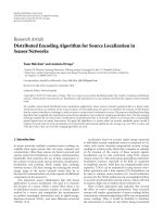
Figure 3: The convergence of parameter estimates n
t
(a), n
p
(b),

k
1
(c), and

k
−1
(d) as a function of the number of iterations of the Gibbs
sampler.
exploiting the linearity of our SDE model, the scaled down
continuous-discrete model is given by
d
n
c
(
t
)
= μ
(
n
c

, θ, t
)
dt + σ
(
n
c
, θ, t
)
dW,
y
(
t
)
= n
c
(
t
)
+
v
(
t
)
,
(46)
where
n
c
= n
c

/k, v = v/k, y = y/k,and
μ = k
1
n
p
−n
c
n
p
(
n
t
−n
c
)
−k
−1
n
c
,
σ =

k
1
n
p
−n
c
n
p

(
n
t
−n
c
)
+ k
−1
n
c

1/2
,
(47)
where
n
p
= n
p
/k and n
t
= n
t
/k.
Moreover, since the noise variance is generally unknown,
we add it to the vector of the unknown parameters, that is,
θ
= [n
t
n

p
k
1
k
−1
]. This requires slight modification in
the step 3 of the MCMC algorithm (as described previously).
We applied the proposed Gibbs Sampler to the estimation
of the parameters of the process which generated the
described experimental data. We run 5000 iterations of the
algorithm with M
= 5andK = 1500, and averaged its
performance over 50 trials. For the first experiment, we
obtained
n
t,1
= 3.3 × 10
8
, while in the second experiment
n
t,2
= 1.1 × 10
8
. Figure 3 and 4 show a sample convergence
of the parameter estimates as a function of the number of
iterations of the Gibbs sampler applied to the second data
0
2
4
6

8
10
12
14
16
18
×10
5
0 1000 2000 3000 4000 5000
Iteration number of Gibbs sampler
Variance of measurement noise
Figure 4: The convergence of the noise variance estimate as a
function of the number of iterations of the Gibbs sampler.
set. We note that the ratio of the estimated target amounts is
n
t,1
/n
t,2
= 3, which is close to the true ratio of 80ng/16ng =
5. On the other hand, unable to observe the kinetics of
the hybridization process conventional microarrays would
simply estimate the ratio of target molecules by the ratio of
captured molecules at the end of the experimental run. For
the experiments under consideration, this ratio is 2.77.
8 EURASIP Journal on Advances in Signal Processing
7. Summary and Conclusion
In this paper, we considered the problem of estimating
the number of target molecules in stochastically modeled
biomolecular sensors. We posed it as a parameter estima-
tion problem in systems modeled by stochastic differential

equations, where the noise-perturbed data is acquired at
discrete points in time. Since the problem is analytically
intractable, we employed MCMC techniques to obtain a
numerical solution. In particular, we relied on the use of
the Gibbs Sampler to alternate between drawing missing
data conditioned on parameters and observations, and
drawing parameters conditioned on the simulated missing
data and the observations. We used the Metropolis-Hastings
technique within the Gibbs Sampler to simulate analytically
untractable densities. Simulation results indicate that the
proposed algorithm significantly outperforms the existing
least-mean-squares approach, and that the algorithm is
robust with respect to the measurement noise. Moreover,
we applied the algorithm to experimental data to verify the
validity of the estimation algorithm in a realistic scenario.
There are several possible extensions of the current
work. For instance, the MCMC algorithm described in this
paper can also be applied to multivariate diffusion processes.
Such processes arise in the context of gene regulatory
network as well as in real-time biosensor arrays affected
by cross-hybridization. For this scenario, one may extend
the algorithm so that it handles unobserved parts of a
multivariate diffusion process. On another note, a variation
of the MCMC algorithm performs (random) block updating
(see, e.g., [19, 20]). It is worth pursuing this modification in
the context of parameter estimation in real-time biosensors.
References
[1] J. Cooper and T. Cass, Eds., Biosensors, Oxford University
Press, Oxford, UK, 2nd edition, 2004.
[2] K. R. Rogers and A. Mulchandani, Affinity Biosensors, Humana

Press, Totowa, NJ, USA, 1998.
[3] K.R.M.Schena,Microarray Analysis, John Wiley & Sons, New
York Ny, USA, 2003.
[4] L. Shi, L. H. Reid, W. D. Jones et al., “The MicroArray Quality
Control (MAQC) project shows inter- and intraplatform
reproducibility of gene expression measurements,” Nature
Biotechnology, vol. 24, no. 9, pp. 1151–1161, 2006.
[5] E. Marshall, “Getting the noise out of gene arrays,” Sc ience, vol.
306, no. 5696, pp. 630–631, 2004.
[6] S. Draghici, P.Khatri, A. C. Eklund, and Z. Szallasi, “Reliability
and reproducibility issues in DNA microarray measurements,”
Trends in Genetics, vol. 22, no. 2, pp. 101–109, 2006.
[7] D. I. Stimpson, J. V. Hoijer, W. Hsieh et al., “Real-time
detection of DNA hybridization and melting on oligonu-
cleotide arrays by using optical wave guides,” Proceedings of the
National Academy of Sciences of the United States of America,
vol. 92, no. 14, pp. 6379–6383, 1995.
[8] J. Bishop, A. M. Chagovetz, and S. Blair, “Kinetics of multiplex
hybridization: mechanisms and implications,” Biophysical
Journal, vol. 94, no. 5, pp. 1726–1734, 2008.
[9]M.R.Henry,P.W.Stevens,J.Sun,andD.M.Kelso,“Real-
time measurements of DNA hybridization on microparticles
with fluorescence resonance energy transfer,” Analytical Bio-
chemistry, vol. 276, no. 2, pp. 204–214, 1999.
[10] V. M. Mirsky, “Affinity sensors in non-equilibrium conditions:
highly selective chemosensing by means of low selective
chemosensors,” Sensors, vol. 1, no. 1, pp. 13–17, 2001.
[11] H. Vikalo, B. Hassibi, and A. Hassibi, “Modeling and estima-
tion for real-time microarrays,” IEEE Journal on Selected Topics
in Signal Processing, vol. 2, no. 3, pp. 286–296, 2008.

[12] S. Das, H. Vikalo, and A. Hassibi, “On scaling laws of
biosensors: a stochastic approach,” Journal of Applied Physics,
vol. 105, no. 10, Article ID 102021, 2009.
[13] E. Allen, Modeling with It
ˆ
oStochasticDifferential Equations,
Springer, New York, NY, USA, 2007.
[14] H. Sørensen, “Parametric inference for diffusion processes
observed at discrete points in time: a survey,” International
Statistical Review, vol. 72, no. 3, pp. 337–354, 2004.
[15] B. M. Bibby, “Estimating functions for discretely sampled dif-
fusion type models,” in Handbook of Financial Econometrics,
North-Holland, Amsterdam, The Netherlands, 2002.
[16] A. R. Gallant and J. R. Long, “Estimating stochastic differential
equations efficiently by minimum chi-squared,” Biometrika,
vol. 84, no. 1, pp. 125–141, 1997.
[17] B. Eraker, “MCMC analysis of diffusion models with appli-
cation to finance,” Journal of Business and Economic Statistics,
vol. 19, no. 2, pp. 177–191, 2001.
[18] G. O. Roberts and O. Stramer, “On inference for partially
observed nonlinear diff
usion models using the Metropolis-
Hastings algorithm,” Biometrika, vol. 88, no. 3, pp. 603–621,
2001.
[19] A. Golightly, Bayesian inference for nonlinear multivariate dif-
fusion processes, Ph.D. thesis, Newcastle University, Newcastle,
UK, 2006.
[20] O. Elerian, S. Chib, and N. Shephard, “Likelihood inference for
discretely observed nonlinear diffusions,” Econometrica, vol.
69, no. 4, pp. 959–993, 2001.

[21] Y. A
¨
ıt-Sahalia, “Maximum likelihood estimation of discretely
sampled diffusions: a closed-form approximation approach,”
Econometrica, vol. 70, no. 1, pp. 223–262, 2002.
[22] A. W. Lo, “Maximum likelihood estimation of generalized Ito
processes with discretely sampled data,” Econometric Theory,
vol. 4, pp. 231–247, 1988.
[23] R. Poulsen, “Approximate maximum likelihood estimation of
discretely observed diffusion processes,” Tech. Rep. 29, Centre
for Analytical Finance, University of Aarhus, 1999.
[24] A. R. Pedersen, “A new approach to maximum likelihood
estimation for stochastic differential equations based on
discrete observations,” Scandinavian Journal of Statistics, vol.
22, pp. 55–71, 1995.
[25] J. C. Spall, “Estimation via Markov chain Monte Carlo,” IEEE
Control Systems Magazine, vol. 23, no. 2, pp. 34–45, 2003.
[26] B. Oksendal, Stochastic Differential Equations: An Introduction
with Applications, Springer, Berlin, Germany, 2003.
[27] J. P. N. Bishwal, Parameter Estimation in Stochastic Differential
Equations, Springer, New York, NY, USA, 2007.
[28] P. Kloeden and E. Platen, Numeric Solutions of Stochastic
Differential Equations, Springer, New York, NY, USA, 1992.
[29] M. W. Brandt and P. Santa-Clara, “Simulated likelihood
estimation of diffusions with an application to exchange
rate dynamics in incomplete markets,” Journal of Financ ial
Economics, vol. 63, no. 2, pp. 161–210, 2002.
[30] G. B. Durham and A. R. Gallant, “Numerical techniques for
maximum likelihood estimation of continuous-time diffusion
processes,” Journal of Business and Economic Statistics, vol. 20,

no. 3, pp. 297–316, 2002.