Báo cáo hóa học: " Research Article Distributed Encoding Algorithm for Source Localization in Sensor Networks" potx

Hindawi Publishing Corporation
EURASIP Journal on Advances in Signal Processing
Volume 2010, Article ID 781720, 13 pages
doi:10.1155/2010/781720
Research Article
Distributed Encoding Algorithm for Source Localization in
Sensor Networks
Yo on Ha k Ki m
1
and Antonio Orteg a
2
1
System LSI Division, Samsung Electronics, Giheung campus, Gyeonggi-Do 446-711, Republic of Korea
2
Department of Electrical Engineering, Signal and Image Processing Institute, University of Southern California,
Los Angeles, CA 90089-2564, USA
Correspondence should be addressed to Yoon Hak Kim,
Received 12 May 2010; Accepted 21 September 2010
Academic Editor: Erchin Serpedin
Copyright © 2010 Y. H. Kim and A. Ortega. This is an open access article distributed under the Creative Commons Attribution
License, which permits unrestricted use, distribution, and reproduction in any medium, provided the original work is properly
cited.
We consider sensor-based distributed source localization applications, where sensors transmit quantized data to a fusion node,
which then produces an estimate of the source location. For this application, the goal is to minimize t he amount of information
that the sensor nodes have to exchange in order to attain a certain source localization accuracy. We propose a distributed encoding
algorithm that is applied after quantization and achieves significant rate savings by merging quantization bins. The bin-merging
technique exploits the fact that certain combinations of quantization bins at each node cannot occur because the corresponding
spatial regions have an empty intersection. We apply the algorithm to a system where an acoustic amplitude sensor model is
employed at each node for source localization. Our experiments demonstrate significant rate savings (e.g., over 30%, 5 nodes, and
4 bits per node) when our novel bin-merging algorithms are used.
1. Introduction

In sensor networks, multiple correlated sensor readings are
available from many sensors that can sense, compute and
communicate. Often these sensors are battery-powered and
operate under strict limitations on wireless communication
bandwidth. This motivates the use of data compression in
the context of various tasks such as detection, classification,
localization, and tracking, which require data exchange
between sensors. The basic strateg y for reducing the overall
energy usage in the sensor network would then be to
decrease the communication cost at the expense of additional
computation in the sensors [1].
One important sensor collaboration task with broad
applications is source localization. The goal is to estimate
the location of a source within a sensor field, where a set
of distributed sensors measures acoustic or seismic signals
emitted by a source and manipulates the measurements
to produce meaningful information such as signal energy,
direction-of-arrival (DOA), and time difference-of-arrival
(TDOA) [2, 3].
Localization based on acoustic signal energy measured
at individual acoustic amplitude sensors is proposed in [4],
where each sensor transmits unquantized acoustic energy
readings to a fusion node, which then computes an estimate
of the location of the source of these acoustic signals.
Localization can be also performed using DOA sensors
(sensor arrays) [5]. The sensor arrays generally provide better
localization accuracy, especially in far field, as compared
to amplitude sensors, while they are computationally more
expensive. TDOA can b e estimated by using various corre-
lation operations and a least squares (LS) formulation can

be used to estimate source location [6]. Good localization
accuracy for the TDOA method can be accomplished if there
is accurate synchronization among sensors, which will tend
to require a hig h cost in wireless sensor networks [3].
None of these approaches take explicitly into account
the effect of sensor reading quantization. Since practical
systems will require quantization of sensor readings before
transmission, estimation algorithms will be run on quantized
sensor readings. Thus, it would be desirable to minimize
the information in terms of rate before being transmitted
2 EURASIP Journal on Advances in Signal Processing
z
1
Q
1
Q
1
Q
1
E
N
C
ENC
Node 1
z
M
Q
M
Q
M

Q
M
Node M
.
.
.
x
x
Decoder
Fusion node
Localization
algorithm
System for localization in sensor networks
z
1
= f (x, x
1
, P
1
)+ω
1
z
M
= f (x, x
M
, P
M
)+ω
M
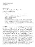
Figure 1: Block diagram of source localization system. We assume that the channel between each node and fusion node is noiseless and each

node sends its quantized (Quantizer, Q
i
) and encoded (ENC block) measurement to the fusion node, where decoding and localization are
conducted in a distributed manner.
to a fusion node. It is noted that there exists some degree
of redundancy between the quantized sensor readings since
each sensor collects information (e.g., signal energy or direc-
tion) regarding a source location. Clearly, this redundancy
can be reduced by adopting distributed quantizers designed
to maximize the localization accuracy by exploiting the
correlation between the sensor readings (see [7, 8]).
In this paper, we observe that the redundancy can be
also reduced by encoding the quantized sensor readings
for a situation, where a set of nodes (Each node may
employ one sensor or an array of sensors, depending on the
applications) and a fusion node wish to cooperate to estimate
a source location (see Figure 1). We assume that each
node can estimate noise-corrupted source charac teristics (z
i
in Figure 1), such as signal energy or DOA, using actual
measurements (e.g., time-series measurements or spatial
measurements). We also assume that there is only one way
communication from nodes to the fusion node; that is, there
is no feedback channel, the nodes do not communicate
with each other (no relay between nodes), and these various
communication links are reliable.
In our problem, a source signal is measured and quan-
tized by a series of distributed nodes. Clearly, in order to
make localization possible, each possible location of the
source produces a different vector of sensor readings at the

nodes. Thus, the vector of the readings (z
1
, , z
M
) should
uniquely define the localization. Quantization of the readings
at each node reduces the accuracy of the localization. Each
quantized value (e.g., Q
i
at node i) of a sensor reading can
then be linked to a region in space, where the source can be
found. For example, if distance information is provided by
Q
j−1
2
Q
j
2
Q
j+1
2
Q
k
3
Q
i−1
1
Q
i
1

Q
i+1
1
Node 1
Node 2
Node 3
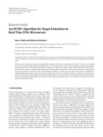
Figure 2: Simple example of source localization, where an acoustic
amplitude sensor is employed at each node. The shaded regions
refer to nonempty intersections, where the source can be found.
sensor readings, the regions corresponding to sensor read-
ings will be circles centered on the nodes and thus quantized
values of those readings will then be mapped to “rings”
centered on the nodes. Figure 2 illustrates the case, where
3 nodes equipped with acoustic amplitude sensors measure
EURASIP Journal on Advances in Signal Processing 3
the distance information for source localization. Denote
Q
j
i
the jth quantization bin at node i; that is, whenever
sensor reading z
i
at node i belongs to jth bin, the node
will transmit Q
j
i
to the fusion node. From the discussion,
it should be clear that since each quantized sensor reading
Q
i

can be associated with the corresponding ring, the fusion
node can locate the source by computing the intersection
of those 3 rings from the combination (Q
1
, Q
2
, Q
3
)received
from the 3 nodes. (In a noiseless case, there always exists
a nonempty intersection corresponding to each received
combination, where a source i s located. However, empty
intersections may be constructed in a noisy case. In Figure 2,
suppose that node 2 transmits Q
j−1
2
instead of Q
j
2
due
to measurement noise. Then, the fusion node will receive
(Q
i
1
, Q
j−1
2
, Q
k
3

) which leads to an empty intersection. Prob-
abilistic localization methods should be employed to handle
empty intersections. For further details, see [ 9].) Therefore,
the combinations such as (Q
i
1
, Q
j+1
2
, Q
k
3
)or(Q
i
1
, Q
j
2
, Q
k
3
)
transmitted from the nodes will tend to produce nonempty
intersections (the shaded regions in Figure 2, resp.) while
numerous other combinations randomly collected may lead
to empty intersections, implying that such combinations
are very unlikely to be transmitted from the nodes (e.g.,
(Q
i+1
1

, Q
j−1
2
, Q
k
3
), (Q
i−1
1
, Q
j−1
2
, Q
k
3
), and many others). In this
work, we focus on developing tools that allow us to exploit
this observation in order to eliminate the redundancy. More
specifically, we consider a novel way of reducing the effective
number of quantization bins consumed by all the nodes
involved while preserving localization performance. Suppose
that one of the nodes reduces the number of bins that
are being used. This will cause a corresponding increase
of uncertainty. However, the fusion node that receives a
combination of the bins from all the nodes should be able to
compensate for the increase by using the data from the other
nodes as side information.
We propose a novel distributed encoding algorithm that
allows us to achieve significant rate savings [8, 10]. With
our method, we merge (non-adjacent) quantization bins in

a given node whenever we determine that the ambiguity
created by this merging can be resolved at the fusion node
once information from other nodes is taken into account.
In [11], the authors focused on encoding the correlated
measurements by merging the adjacent quantization bins at
each node so as to achieve rate savings at the expense of
distortion. Notice that they search the quantization bins to be
merged that show redundancy in encoding perspective while
we find the bins for merging that produce redundancy in
localization perspective. In addition, while in their approach
each computation of distortion for pairs of bins will be
required to find the bins for merging, we develop simple
techniques that choose the bins to be merged in a systematic
way.
It is noted that our algorithm is an example of binning
as can be found in Slepian-Wolf and Wyner-Ziv techniques
[11, 12]. In our approach, however, we achieve rate savings
purely through binning and provide several methods to
select candidate bins for merging. We apply our distributed
encoding algorithm to a system, where an acoustic amplitude
sensor model proposed in [4] is considered. Our experiments
show rate savings (e.g., over 30%, 5 nodes, and 4 bits per
node) when our novel bin-merging algorithms are used.
This paper is organized as follows. The terminologies
and definitions are given in Section 2, and the motivation
is explained in Section 3.InSection 4,weconsiderquan-
tization schemes that can be used with the encoding at
each node. An iterative encoding algorithm is proposed in
Section 5. For a noisy situation, we consider the modified
encoding algorithm in Section 6 and describe the decoding

process and how to handle decoding errors in Section 7.In
Section 8, we apply our encoding algorithm to the source
localization system, where an acoustic amplitude sensor
model is employed. Simulation results are given in Section 9 ,
and the conclusions are found in Section 10.
2. Terminologies and Definitions
Within the sensor field S of interest, assume that there are
M nodes located at known spatial locations, denoted x
i
, i =
1, , M,wherex
i
∈ S ⊂ R
2
. The nodes measure signals
generated by a source located at an unknown location x
∈ S.
Denote by z
i
the measurement (equivalently, sensor reading)
at the ith node over a time interval k
z
i
(
x, k
)
= f
(
x, x
i

, P
i
)
+ w
i
(
k
)
∀i = 1, , M,(1)
where f (x, x
i
, P
i
) denotes the sensor model employed at
node i and the measurement noise w
i
(k) can be approxi-
mated using a normal distribution, N(0, σ
2
i
). (The sensor
models for acoustic amplitude sensors and DOA sensors
can be expressed in this form [4, 13].) P
i
is the parameter
vector for the sensor model (an example of P
i
for an acoustic
amplitude sensor case is given in Section 8). It is assumed
that each node measures its sensor reading z

i
(x, k)attime
interval k, quantizes it and sends it to a fusion node, where
all sensor readings are used to obtain an estimate
x of the
source location.
At node i, we use a R
i
-bit quantizer with a dynamic range
[z
i,min
z
i,max
]. We assume that the quantization range can be
selected for each node based on desirable properties of their
respective sensing ranges [14]. Denote by α
i
(·) the quantizer
with quantization level L
i
at node i,whichgeneratesa
quantization index Q
i
∈ I
i
={1, ,2
R
i
= L
i

}. In what
follows, Q
i
will be also used to denote the quantization bin
to which m easurement z
i
belongs.
This formulation is general and captures many scenarios
of practical interest. For example, z
i
(x, k) could be the energy
captured by an acoustic amplitude sensor (this will b e the
case study presented in Section 8), but it could also be a
DOA measurement. (In the DOA case, each measurement
at a given node location will be provided by an array of
collocated sensors.) Each scenario will obviously lead to a
different sensor model f (x, x
i
, P
i
). We assume that the fusion
node needs measurements, z
i
(x, k), from all nodes in order to
estimate the source location.
4 EURASIP Journal on Advances in Signal Processing
Let S
M
= I
1

×I
2
×···×I
M
be the cartesian product of the
sets of quantization indices. S
M
contains |S
M
|=(

M
i
L
i
) M-
tuples representing all possible combinations of quantization
indices
S
M
={
(
Q
1
, , Q
M
)
|Q
i
=1, , L

i
, i = 1, , M}. (2)
We denote S
Q
the subset of S
M
that contains all the
quantization index combinations that can occur in a real
system, that is, all those generated as a source moves around
the sensor field and produces readings at each node
S
Q
={
(
Q
1
, , Q
M
)
|∃x ∈ S, Q
i
=α
i
(
z
i
(
x
))
, i

=1, , M}.
(3)
For example, assuming that each node measures noiseless
sensor readings (i.e., w
i
= 0), we can construct the
set S
Q
by collecting only the combinations that lead to
nonempty intersections. (The combinations (Q
i
1
, Q
j+1
2
, Q
k
3
),
(Q
i
1
, Q
j
2
, Q
k
3
) corresponding to the shaded regions in Figure 2
will belong to S

Q
.) In a noisy situation, how to construct S
Q
will be further explained in Section 6.
We den ote S
j
i
the subset of S
Q
that contains all M-tuples
in which the ith node is assigned the jth quantization bin
S
j
i
=

(
Q
1
, , Q
M
)
∈ S
Q
| Q
i
= j

,
i

= 1, , M, j = 1, , L
i
.
(4)
This set will provide all possible combinations of (M
− 1)
tuples that can be transmitted from other nodes when the
jth bin at node i was actually transmitted. In other words,
the fusion node will be able to identify which bin actually
occurred at node i by exploiting the set as side information,
when there is uncertainty induced by merging bins at node i.
Since (M
− 1) quantized measurements out of each M-
tuple in S
j
i
are used in actual process of encoding, it would
be useful to construct the set of (M
− 1) tuples generated
from S
j
i
. We denote by S
j
i
the set of (M − 1)-tuples obtained
from M-tuples in S
j
i
, where only the quantization bins at

positions other than position i are stored. That is, if Q
=
(Q
1
, , Q
M
) = (a
1
, , a
M
) ∈ S
j
i
, then we always have
(a
1
, , a
i−1
, a
i+1
, , a
M
) ∈ S
j
i
. Clearly, there is one to one
correspondence between the elements in S
j
i
and S

j
i
, so that
|S
j
i
|=|S
j
i
|.
3. Motivation: Identifiability
In this section, we assume that Pr[(Q
1
, , Q
M
) ∈ S
Q
] = 1;
that is, only combinations of quantization indices belonging
to S
Q
can occur and those combinations belonging to S
M
−
S
Q
never occur. These sets can be easily obtained when
there is no measurement noise (i.e., w
i
= 0) and no

parameter mismatches. As discussed in the introduction,
there will be numerous elements in S
M
thatarenotinS
Q
.
Therefore, simple scalar quantization at each node would be
inefficient because a standard scalar quantizer would allow
us to represent any of the M-tuples in S
M
. What we would
like to determine now is a method such that independent
quantization can still be performed at each node, while at the
same time, we reduce the redundancy inherent in allowing all
the combinations in S
M
to be chosen. Note that, in general,
determining that a specific quantizer assignment in S
M
does
not belong to S
Q
requires having access to the whole vector,
which obviously is not possible if quantization has to be
performed independently at each node.
In our design, we will look for quantization bins in a
given node that can be merged without affecting localization.
As will be discussed next, this is because the ambiguity
created by the merger can be resolved once information
obtained from the other nodes is taken into account. Note

that this is the basic principle behind distributed source
coding techniques: binning at the encoder, which can be
disambiguated once side information is made available at the
decoder [11, 12, 15] (in this case, quantized values from other
nodes).
Merging of bins results in bit rate savings because fewer
quantization indices have to be transmitted. To quantify the
bit rate savings, we need to take into consideration that
quantization indices will be entropy coded (in this paper,
Huffman coding is used). Thus, when evaluating the possible
merger of two bins, we will compute the probability of the
merged bin as the sum of the probabilities of the bins merged.
Suppose that Q
j
i
and Q
k
i
are merged into Q
min( j,k)
i
. Then, we
can construct the set S
min(j,k)
i
and compute the probability for
the merged bin as follows:
S
min(j,k)
i

= S
j
i
∪ S
k
i
,
P
min(j,k)
i
= P
j
i
+ P
k
i
,
(5)
where P
j
i
=

x∈A
j
i
p(x)dx, p(x) is the pdf of the source
position and A
j
i

is given by
A
j
i
=

x|
(
Q
1
=α
1
(
z
1
(
x
))
, , Q
M
=α
M
(
z
M
(
x
)))
∈S
j

i

. (6)
Since the encoder at node i merges Q
j
i
and Q
k
i
into Q
l
i
with l = min(j, k), it sends the corresponding index, l to
the fusion node whenever the sensor reading belongs to Q
j
i
or Q
k
i
. The decoder will try to determine which of the two
merged bins (Q
j
i
or Q
k
i
in this case) actually occurred at node
i. To do so, the decoder will use the information provided by
the other nodes, that is, the quantization indices Q
m

(m
/
= i).
Consider one particular source position x
∈ S for which
node i produces Q
j
i
and the remaining nodes produce a
combination of M
−1 quantization indices Q ∈ S
j
i
. (To avoid
confusion, we denote Q avectorofM quantization indices
and
Q avectorofM-1 quantization indices, resp.) Then, for
this x there would be no ambiguity at the decoder, even if bins
Q
j
i
and Q
k
i
were to be merged, as long as Q
/
∈ S
k
i
. This follows

because if Q
/
∈ S
k
i
the decoder would be able to determine
that only Q
j
i
is consistent with receiving Q. With the notation
adopted earlier this leads to the following definition:
EURASIP Journal on Advances in Signal Processing 5
P(S
Q
) = p
Simple example of merging process (3 nodes, R
i
= 2 bits)
Q
1
Q
2
Q
3
Q
1
Q
2
Q
3

Q
1
Q
2
Q
3
Pr
1
2
2
2
2
2
22
2
2
22
2
2
2
2
3
3
3
33
3
3
3
3
333

3
33
3
3
3
3
3
333
1
P
1
21
4
4
14
1
1
1
1
1
1
1
11
1
1
1
4
4
4
44

4
4
4
4
4
4
4
44
4
4
P
2
.
.
.
.
.
.
.
.
.
.
.
.
.
.
.
.
.
.

K +1
P
K+1
Pr(Q
1
, Q
2
, Q
3
) = 1 − p
63 1 1 1 P
63
64 1 1 2
P
64
K combinations of
quantization indices
are rearranged
Canbemerged
≥ identifiable
Send quantization index 1 whenever z
1
belongs to the
first bin or the fourth bin. −→ rate saving achieved
Sorted by its probability
in a descending order: P
i
≥ P
j
if i <j

S
1
1
S
1
1
∪
S
4
1
S
4
1
= ∅
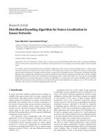
Figure 3: Simple example of m erging process, where there are 3 nodes and each node uses a 2 bit quantizer (Q
i
∈{1, 2, 3,4}). In this case, it
is assumed that Pr(S
M
− S
Q
) = 1 − p ≈ 0.
Definition 1. Q
j
i
and Q
k
i
are identifiable, and therefore can be
merged, if and only if

S
j
i
∩ S
k
i
=∅.
Figure 3 illustrates how to merge quantization bins for
a simple case, where there are 3 nodes deployed in a sensor
field. It is noted that the first bin Q
1
1
(equivalently, Q
1
= 1)
and the fourth bin Q
4
1
at node 1 can be merged since the
sets
S
1
1
and S
4
1
have no elements in common. This merging
process will be repeated in the other nodes until there are no
quantization bins that can be merged.
4. Quantization Schemes

As mentioned in the previous section, there will be
redundancy in M-tuples after quantization which can be
eliminated by our merging technique. However, we can
also attempt to reduce the redundancy during quantizer
design before the encoding of the bins is performed. Thus,
it would be worth considering the effect of selection of a
given quantization scheme on system performance when the
merging technique is employed. In this section, we consider
three schemes as follows.
(i) Uniform quantizers. Since they do not utilize any statistics
about the sensor readings for quantizer design, there will
be no reduction in redundancy by the quantization scheme.
Thus only the merging technique plays a role in improving
the system performance.
(ii) L1oyd quantizers. Using the statistics about the sensor
reading z
i
available at node i, the ith quantizer α
i
is designed
using the generalized L1oyd algor i thm [16] with the cost
function
|z
i
− z
i
|
2
which is minimized in an iterative fashion.
Since each node consider only the information available

to it during quantizer design, there will still exist much
redundancy after quantization which the merging technique
can attempt to reduce.
(iii) Localization specific quantizers (LSQs) proposed in [7].
While desig ning a quantizer at node i, we can take into
account the effect of quantized sensor readings at other
nodes on the quantizer design by introducing the localization
error in a new cost function, which will be minimized in an
iterative manner. ( The new cost function to be minimized
is expressed as the Lagrangian functional
|z
i
− z
i
|
2
+ λx −

x
2
. The topic of quantizer design in distributed setting
goes beyond the scope of this work. See [7, 8]fordetailed
information.) Since the correlation between sensor readings
is exploited during quantizer design, LSQ along with our
merging technique will show the best performance of all.
We will discuss the effect of quantization and encoding
on the system performance based on experiments for an
acoustic amplitude sensor system in Section 9.1.
5. Proposed Encoding Algorithm
In general, there will be multiple pairs of identifiable

quantization bins that can be merged. Often, all candidate
6 EURASIP Journal on Advances in Signal Processing
identifiable pairs cannot be merged simultaneously; that
is, after a pair has been merged, other candidate pairs
may become nonidentifiable. In what follows, we propose
algorithms to determine in a sequential manner which pairs
should be merged.
In order to minimize the total rate consumed by
M nodes, an optimal merging technique should attempt to
reduce the overall entropy as much as possible, which can be
achieved by (1) merging high probability bins together and
(2) merging as many bins as possible. It should be observed
that these two strategies cannot be pursued simultaneously.
This is because high probability bins (under our assumption
of uniform distribution of the source position) are large and
thus merging large bins tends to result in fewer remaining
merging choices (i.e., a larger number of identifiable bin
pairs may become nonidentifiable after two large identifiable
bins have been merged). Conversely, a strategy that tries to
maximize the number of merged bins will tend to merge
many smal l bins, leading to less significant reductions in
overall entropy. In order to strike a balance between these
two strategies, we define a metric, W
j
i
, attached to each
quantization bin
W
j
i

= P
j
i
− γ



S
j
i



,(7)
where γ
≥ 0. This is a weighted sum of the bin probability
and the number of the combinations of M-tuples that
include Q
j
i
. If P
j
i
is large the corresponding bin would be a
good candidate for merging under criterion (1) whereas a
small value of
|S
j
i
| will indicate a good choice under criterion

(2). In our proposed procedure, for a suitable value of γ,
we will seek to prioritize the merging of those identifiable
bins having the largest total weighted metric. This will be
repeated iteratively until there are no identifiable bins left.
The selection of γ can be heuristically made so as to minimize
the total rate. For example, several different γ’s could be
evaluated in (7) to first determine its applicable range which
will be then searched to find a proper value of γ. Clearly, γ
depends on the application.
The proposed global merging algorithm is summarized as
follows.
Step 1. Set F(i, j)
= 0, where i = 1, , M; j = 1, , L
i
,
indicating that none of the bins, Q
j
i
,havebeenmergedyet.
Step 2. Find (a, b)
= arg max
(i, j)|F(i, j)=0
(W
j
i
), that is, we
search over all the nonmerged bins for the one with the
largest metric W
b
a

.
Step 3. Find Q
c
a
, c
/
= b such that W
c
a
= max
j
/
= b
(W
j
a
), where
the search for the maximum is done only over the bins
identifiable with Q
b
a
at node a and go to Step 4. If there
are no bins identifiable with Q
b
a
,setF(a, b) = 1, indicating
the bin Q
b
a
is no longer involved in the merging process. If

F(i, j)
= 1, for all i, j, stop; otherwise, go to Step 2.
Step 4. Merge Q
b
a
and Q
c
a
to Q
min(b,c)
a
with S
min(b,c)
a
= S
b
a
∪ S
c
a
.
Set F(a,max(b, c))
= 1. Go to Step 2.
In the proposed algorithm, the search for the maximum
of the metric is done for the bins of all nodes involved.
However , different approaches can be considered for the
search. These are explained as follows.
Method 1 (Complete sequential merging). In this method, we
process one node at a time in a specified order. For each node,
we merge the maximum number of bins possible before

proceeding to the next node. Merging decisions are not
modified once made. Since we exhaust all possible mergers
in each node, after scanning al l the nodes no more additional
mergers are possible.
Method 2 (Partial sequential merging). In this method, we
again process one node at a time in a specified order. For
each node, among all possible bin mergers, the best one
according to a criterion is chosen (the criterion could be
entropy based and e.g., (7) is used in this paper) and after
the chosen bin is merged we proceed to the next node. This
process is continued until no additional mergers are possible
in any node. This may require multiple passes through the
set of nodes.
These two methods can be easily implemented with
minor modifications to our proposed algorithm. Notice that
the final result of the encoding algorithm will be M merging
tables, each of which has the information about which bins
canbemergedateachnodeinrealoperation.Thatis,each
node will merge the quantization bins using the merging
table s tored at the node and will send the merged bin to the
fusion node which then tries to determine which bin actually
occurred via the decoding process using M merging tables
and S
Q
.
5.1. Incremental Merging. The complexity of the above
procedures is a function of the total number of quantization
bins, and thus of the number of the nodes involved.
These approaches could potentially be complex for large
sensor fields. We now show that incremental merging is

possible; that is, we can start by performing the merging
based on a subset consisting of N sensor nodes, N <
M, and it can be guaranteed that the merging decisions
that were valid when N nodes were considered will remain
validevenwhenallM nodes are taken into account. To
see this, suppose that Q
j
i
and Q
k
i
are identifiable when
only N nodes are considered. From Definition 1,
S
j
i
(N) ∩
S
k
i
(N) =∅,whereN indicates the number of nodes
involved in the merging process. Note that since every
element Q
j
(M) = (Q
1
, , Q
N
, Q
N+1

, , Q
M
) ∈ S
j
i
(M)(In
thissection,wedenotebyQ
j
(M) an element (Q
1
, , Q
i
=
j, , Q
M
) ∈ S
j
i
(M). Later, it will be also used to denote
an jth element in S
Q
in Section 8 without confusion) is
constructed by concatenating M
− N indices Q
N+1
, , Q
M
with the corresponding element, Q
j
(N) = (Q

1
, , Q
N
) ∈
S
j
i
(N), we have that Q
j
(M)
/
= Q
k
(M)ifQ
j
(N)
/
= Q
k
(N). By
the property of the intersection operator
∩, we can claim
that
S
j
i
(M) ∩ S
k
i
(M) =∅for all M ≥ N, implying that Q

j
i
and Q
k
i
are still identifiable even w hen we consider M nodes.
EURASIP Journal on Advances in Signal Processing 7
Thus, we can start the merging process with just two nodes
and continue to do further merging by adding one node (or
a few) at a time without change in previously merged bins.
When many nodes are involved, this would lead to significant
savings in computational complexity. In addition, if some of
the nodes are located far away from the nodes being added
(i.e., the dynamic ranges of their quantizers do not overlap
with those of the nodes being added), they can be skipped
for further merging without loss of merging performance.
6. Extension of Identifiability:
p-Identifiability
Since for real operating conditions, there exist measurement
noise (w
i
/
= 0) and/or parameter mismatches, it is com-
putationally impractical to construct the set S
Q
satisfying
the assumption of Pr[Q
∈ S
Q
] = 1 under which the

merging algorithm was derived in Section 3.Instead,we
construct S
Q
(p) such that Pr[Q ∈ S
Q
(p)] = p( 1) and
propose an e xtended version of identifiability thatallowsus
to still apply the merging technique under noisy situations.
With this consideration, Definition 1 can be extended as
follows.
Definition 2. Q
j
i
and Q
k
i
are p-identifiable, and therefore
can be merged, if and only if
S
j
i
(p) ∩ S
k
i
(p) =∅,where
S
j
i
(p)andS
k

i
(p)areconstructedfromS
Q
(p)asS
j
i
from S
Q
in
Section 2. Obviously, to maximize the rate gain achie v able
by the merging technique, we need to construct S
Q
(p)
as small as possible given p. Ideally, we can build the set
S
Q
(p) by collecting the M-tuples with high probability
although it would require huge computational complexity
especially when many nodes are involved at high rates. In
this work, we suggest following the procedure stated below
for construction of S
Q
(p) with reduced complexity.
Step 1. Compute the interval I
z
i
(x) such that P(z
i
∈ I
z

i
(x) |
x) = p
1/M
= 1 − β,foralli. Since z
i
∼ N(f
i
, σ
2
i
), where
f
i
= f (x, x
i
, P
i
)in(1), we can construct the interval
that is symmetr ic w ith respect to f
i
; that is, I
z
i
(x) =
[ f
i
− z
β/2
f

i
+ z
β/2
], so that

M
i
Pr(z
i
∈ I
z
i
(x) | x) = p.
Notice that z
β/2
is determined by σ
i
and β (not a function of
x). For example, if (1
− β) = 0.99, z
β/2
is given by 3σ
i
and
p
= (1 − β)
M
= 0.95 with M = 5.
Step 2. From M intervals I
z

i
(x), i = 1, , M, we generate
possible M-tuples Q
= [Q
1
, , Q
M
] satisfying that Q
i

I
z
i
/
=∅,foralli. Denote by S
Q
(x) a set containing such M
tuples. It is noted that the process of generating M-tuples
from M intervals is deterministic, given M quantizers.
(Simple programming allows us to generate M-tuples
from M intervals. For example, suppose that M
= 3and
I
z
1
= [1.22.3], I
z
2
= [2.73.3], and I
z

3
= [1.83.1] are
computed given x in Step 1.PickanM-tuple Q
∈ S
M
with
Q
1
= [1.52.2], Q
2
= [2.53.1], and Q
3
= [2.12.8].
Then, we determine whether or not Q
∈ S
Q
(x) by
checking Q
i

I
z
i
/
=∅,foralli. In this example, we have
Q
∈ S
Q
(x).)
Step 3. Construct S

Q
(p) =

x∈S
S
Q
(x). We have Pr(Q ∈
S
Q
(p)) = E
x
[Pr(Q ∈ S
Q
(p) | x)] ≈ E
x
[

M
i
Pr(z
i
∈ I
z
i
(x) |
x)] = p.
As β approaches 1, S
Q
(p) will be asymptotically reduced
to S

Q
, the set constructed in a noiseless case. It should be
mentioned that this procedure provides a tool that enables us
to change the size of S
Q
(p) by simply adjusting β. Obviously,
computation of Pr(Q
| x) is unnecessary.
Notice that all the merged bins are p-identifiable (or
identifiable) at the fusion node as long as the M-tuple to be
encoded belongs to S
Q
(p)(orS
Q
). In other words, decoding
errors will be generated when elements in S
M
− S
Q
(p)occur
and there will be tradeoff between rate savings and decoding
errors. If we choose p to be as small as possible, yielding
a small set S
Q
(p), we can achieve good rate savings at the
expense of large decoding error (equivalently, Pr[Q
∈ S
M
−
S

Q
(p)] large), which could lead to degradation of localization
performance. Handling of decoding errors will be discussed
in Section 7 .
7. Decoding of Merged Bins and
Handling Decoding Errors
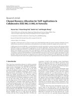
In the decoding process, the fusion node will first decom-
pose the received M-tuple Q
r
into the possible M-tuples,
Q
D
1
, , Q
D
K
by using the M merging tables (see Figure 4).
Note that the merging process is done offline in a centralized
manner. In real operation, each node stores its merging table
which is constructed from the proposed merging algorithm
and used to perform the encoding and the fusion node uses
S
Q
(p)andM merging tables to do the decoding. Revisit
the simple case in Figure 3. According to node 1’s merging
table, Q
1
1
and Q
4

1
can b e merged into Q
1
1
, implying that
node 1 will transmit Q
1
1
to the fusion node whenever z
1
belongs to Q
1
1
or Q
4
1
. Suppose that the fusion node receives
Q
r
= (1,2,4). Then, it decomposes (1, 2, 4) into (1, 2,4) and
(4, 2, 4) by using node 1’s merging table. This decomposition
will be performed for the other M
− 1 merging tables. Note
that (1, 2, 4) is discarded since it does not belong to S
Q
(p),
implying that Q
4
1
actually occurred at node 1.

Suppose that we have a set of K M-tuples, S
D
=
{
Q
D
1
, , Q
D
K
} decomposed from Q
r
via M merging tables.
Then, clearly, Q
r
∈ S
D
and Q
t
∈ S
D
,whereQ
t
is the
true M-tuple before encoding (see Figure 4). Notice that if
Q
t
∈ S
Q
(p), then all merged bins would be identifiable at

the fusion node; that is, after decomposition, there is only
one decomposed M-tuple, Q
t
belonging to S
Q
(p), (As the
decomposition is processed, all the decomposed M-tuples
except Q
t
will be discarded since they do not belong to
S
Q
(p).) and we declare decoding successful. Otherwise, we
declare decoding errors and a pply the decoding rules which
will be explained in the following subsections, to handle
those errors. Since the decoding error occurs only when
Q
t
/
∈ S
Q
(p), the decoding error probability will be less than
1
− p.
It is observed that since the decomposed M-tuples are
produced via the M merging tables from Q
t
,itisverylikely
that Pr(Q
D

k
)  Pr(Q
t
), where Q
D
k
/
= Q
t
, k = 1, , K.
8 EURASIP Journal on Advances in Signal Processing
f
1
Q
1
ENC
ENC
f
M
Q
M
M encoders
x
ZQ
t
Q
E
Q
r
= Q

E
.
.
.
.
.
.
.
.
.
.
.
.
Noiseless
channel
Recoding
rule
decompo-
sition via
merging
tables
Q
D
Q
D
1
Q
D
K
One decoder at fusion node

Figure 4: Encoder-decoder diagram: the decoding process consists of decomposition of the encoded M-tuple Q
E
and decoding rule of
computing the decoded M-tuple Q
D
which will be forwarded to the localization routine.
In other words, since the encoding process merges the
quantization bins whenever any M-tuples that contain either
of them are very unlikely to happen at the same time, the M-
tuples Q
D
k
(
/
= Q
t
) tend to take very low probability.
7.1. Decoding Rule 1: Simple Maximum Rule. Since the
received M-tuple Q
r
has ambiguity produced by encoders at
each node, the decoder at fusion node should be able to find
the true M-tuple by using appropriate decoding rules. As a
simple rule, we can take the M-tuple (out of Q
D
1
, , Q
D
K
)

that is m ost likely to happen. Formally,
Q
D
= arg max
k
Pr

Q
D
k

, k = 1, , K,(8)
where Q
D
is the decoded M-tuple which will be forwarded to
the localization routine.
7.2. Decoding Rule 2: Weighted Decoding Rule. Instead of
choosing only one decoded M-tuple, we can treat each
decomposed M-tuple as a candidate for the decoded M-
tuple, Q
D
with its corresponding weight obtained from the
likelihood. That is, we can view Q
D
k
as one decoded M-tuple
with weight W
k
= Pr[Q
D

k
]/

K
l
Pr[Q
D
l
] k = 1, , K. It
should be noted that the weighted decoding rule should be
used along with the localization routine as follows:
x =
K

k=1
x
k
W
k
k = 1, , K,(9)
where
x
k
is the estimated source location assuming Q
D
=
Q
D
k
. For simplicity, we can take a few dominant M-tuples

5 6 7 8 9 1011121314
Total rate consumed by 5 nodes
0
2
4
6
8
10
12
14
Average localization error (m
2
)
Uniform Q
Lloyd Q
LSQ
Figure 5: Average localization error versus total rate R
M
for
three different quantization schemes with distributed encoding
algorithm. Average rate savings is achieved by the distributed
encoding algorithm (global merging algorithm).
for the weighted decoding and localization
x =
L

k
x
(k)
W

(k)
k = 1, , L, (10)
EURASIP Journal on Advances in Signal Processing 9
2 2.5 3 3.5 4
16
18
20
22
24
26
28
30
32
34
36
Number of bits assigned to each
node, R
i
with M = 5
Averate rate savings
(a)
Averate rate savings
3 3.5 4 4.5 5
10
12
14
16
18
20
22

24
26
28
Number of nodes involved,
M with R
i
= 3
(b)
Figure 6: Average rate savings achieved by the distributed encoding algorithm (g lobal merging algorithm) versus number of bits, R
i
with
M
= 5 (left) and number of nodes with R
i
= 3(right).
where W
(k)
is the weight of Q
D
(k)
and Pr[Q
D
(i)
] ≥ Pr[Q
D
(j)
]
if i < j. Typically, L(<K) is chosen as a small number (e.g.,
L
= 2 in our experiments). Note that the weighted decoding

rule with L
= 1 is equivalent to the simple maximum rule in
(8).
8. Application to Acoustic Amplitude
Sensor Case
As an example of the application, we consider the acoustic
amplitude sensor system, where an energy decay model
of sensor signal readings proposed in [4]isusedfor
localization. The energy decay model was verified by the field
experiment in [4] and was also used in [9, 13, 17].) This
model is based on the fact that the acoustic energy emitted
omnidirectionally from a sound source will attenuate at
a rate that is inversely proportional to the square of the
distance in free space [18]. When an acoustic sensor is
employed at each node, the signal energy measured at node
i over a given time interval k, and denoted by z
i
,canbe
expressed as follows:
z
i
(
x, k
)
= g
i
a
x − x
i


α
+ w
i
(
k
)
, (11)
where the parameter vector P
i
in (1) consists of the gain
factor of the ith node g
i
,anenergydecayfactorα,which
is approximately equal to 2 in free space, and the source
signal energy a. The measurement noise term w
i
(k)can
be approximated using a normal distribution, N(0, σ
2
i
). In
(11), it is assumed that the signal energ y, a, is uniformly
distributed over the range [a
min
a
max
].
In order to perform distributed encoding at each node,
we first need to obtain the set S
Q

, which can be constructed
from (3) as follows:
S
Q
=

(
Q
1
, , Q
M
)
|∃x ∈ S, Q
i
= α
i

g
i
a
x − x
i

α
+ w
i

,
(12)
where the i th sensor reading z

i
(x) is expressed by the sensor
model g
i
(a/x − x
i

α
), and the measurement noise, w
i
.
When the signal energy a is known, and there is no
measurement noise (w
i
= 0), it would be straightforward to
construct the set S
Q
. That is, each element in S
Q
corresponds
to one region in sensor field which is obtained by computing
the intersection of M ring-shaped areas (see Figure 2). For
example, using an j th element Q
j
= (Q
1
, , Q
M
)inS
Q

,we
can compute the corresponding intersection A
j
as follows:
A
i
=

x | g
i
a
x − x
i

α
∈ Q
i
,x∈ S

, i = 1, , M,
A
j
=
M

i
A
i
.
(13)

10 EURASIP Journal on Advances in Signal Processing
40 50 60 70 80 90 100
SNR (R
i
= 3) with M = 5(σ = 0.5)
(σ ≈ 0)
0
5
10
15
20
25
30
35
Rate savings (%)
Pr [decoding error] = 0.0498
Pr [decoding error] = 0.0202
Pr [decoding error] = 0.0037
Rate savings (%) versus SNR w hen R
i
= 3 bits with M = 5
Figure 7: Rate savings achieved by the distributed encoding
algorithm (global merging algorithm) versus SNR (dB) with R
i
= 3
and M
= 5.σ
2
= 0, ,0.5
2

.
Table 1: Total rate, R
M
in bits (rate savings) achieved by various
merging techniques.
R
i
Method 1 M ethod 2 Method 3
2 9.4 (8.7%) 9.4 (8.7%) 9.10 (11.6%)
3 11.9 (20.6%) 12.1 (19.3%) 11.3 (24.6%)
4 13.7 (31.1%) 14.1 (29.1%) 13.6 (31.6%)
Since the nodes involved in localization of any given source
generate the same M-tuple, the set S
Q
will be computed
deterministically and we have Pr[Q
∈ S
Q
] = 1. Thus, using
S
Q
, we can apply our merging technique to this case and
achieve significant rate savings without any degradation of
localization accuracy (no decoding error).
However, measurement noise and/or unknown signal
energy will make this problem complicated by allowing
random realizations of M-tuples generated by M nodes for
any given source location. For this case, we construct S
Q
(p)

by following the procedure in Section 6 and apply our
decoding rules explained in Section 7 to handle decoding
errors.
9. Experimental Results
The distributed encoding algorithm described in Section 5 is
applied to the system, where each node employs an acoustic
amplitude sensor model given by (11) for source localization.
The experimental results are provided in terms of average
localization error. (Clearly, the localization error would be
affected by the estimators employed at the fusion node. The
estimation algorithms go beyond the scope of this work. For
detailed information, see [9].) E
x−x
2
and rate savings (%)
computed by ((R
T
− R
M
)/R
T
) × 100, where R
T
is the rate
Table 2: Total rate R
M
in bits (rate savings) achieved by distributed
encoding algorithm (global merging technique). The rate savings
is averaged over 20 different node configurations, where each node
uses LSQ with R

i
= 3.
M Tot a l rate R
M
in bits (rate savings)
12 17.3237 (51.56%)
16 20.7632 (56.45%)
20 23.4296 (60.69%)
consumed by M nodes when only the independent entropy
coding (Huffman coding) is used after quantization and
R
M
is the rate by M nodes when the merging technique
is applied to quantized data before the entropy coding. We
assume that each node uses LSQ described in Section 4 (for
further details, refer to [7]) except for the experiments where
otherwise stated.
9.1. Distributed Encoding Algorithm: Noiseless Case. It is
assumed that each node can measure the known signal
energy without measurement noise. Figure 5 shows the over-
all performance of the system for each quantization scheme.
In this experiment, 100 different 5-node configurations were
generated in a sensor field 10
×10 m
2
. For each configuration,
a test set of 2000 random source locations was used to obtain
sensor readings, which are then quantized by three different
quantizers, namely, uniform quantizers, L1oyd quantizers,
and LSQs. The average localization error and total rate R

M
are averaged over 100 node configurations. As expected,
the overall performance for LSQ is the best of all since
the total reduction in redundancy can be maximized when
the application-specific quantization such as LSQ and the
distributed encoding are used together.
Our encoding algorithm with the different merging
techniques outlined in Section 5 is applied for comparison,
and the results are provided in Ta ble 1. Methods 1 and 2 are
as described in Section 5, and Method 3 is the global merging
algorithm discussed in that section. We can observe that even
with relative low rates (4 bits per node) and a small number
of nodes (only 5) significant rate gains (over 30%) can be
achieved with our merging technique.
The encoding algorithm was also applied to many dif-
ferent node configurations to characterize the performance.
In this experiment, 500 different node configurations were
generated for each M(
= 3,4, 5) in a sensor field 10 × 10 m
2
.
The global merging technique has been applied to obtain
the rate savings. In computing the metric in (7), the source
distribution is assumed to be uniform. The average rate
savings is plotted by varying M and R
i
in Figure 6. Clearly,
the better rate savings is achieved with larger M and/or at
higher rate since there exists more redundancy expressed as
|S

M
− S
Q
|, as more nodes become involved at higher rate.
Since there are a large number of nodes in typical sensor
networks, our distributed algorithms h ave been applied to
the system in a larger sensor field (20
× 20 m
2
). In this
experiment, 20 different node configurations are generated
for each M(
= 12, 16,20). Note that the node density for
M
= 20 in 20 × 20 m
2
is equal to 20/(20 × 20) = 0.05 which
EURASIP Journal on Advances in Signal Processing 11
8.5 9 9.5 10
1.3
1.4
1.5
1.6
1.7
1.8
1.9
2
2.1
Total rate (bits) consumed by 5 sensors
Localization error (m

2
)
σ = 0.05
σ
= 0
R
i
= 2
(a)
Total rate (bits) consumed by 5 sensors
Localization error (m
2
)
11.5 12 12.5 13 13.5
0.4
0.5
0.6
0.7
0.8
0.9
1
1.1
σ
= 0.05
σ
= 0
R
i
= 3
(b)

Figure 8: Average localization error versus total rate R
M
achieved by the distributed encoding algorithm (global merging algorithm) with
simple maximum decoding and weighted decoding, respectively. Total rate increases by changing p from 0.8to0.95 and weighted decoding
is conducted with L
= 2. Solid line +  : weighted decoding. Solid line + ∇ : simple maximum decoding.
is also the node density for the case of M = 5in10× 10 m
2
.
In Ta ble 2, it is worth noting that the system with a larger
number of nodes outperforms the system with a smaller
number of nodes (M
= 3, 4, 5) although the node density
is kept the same. This is because the incremental property
of the merging technique allows us to find more identifiable
bins at each node.
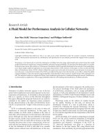
9.2. Encoding with p-Identifiability and Decoding Rules:
Noisy Case. The distributed encoding algorithm with p-
identifiability described in Section 6 was applied to the case,
where each node collects noise-corrupted measurements of
unknown source signal energy. First, assuming known signal
energy, we checked the effect of measurement noise on the
rate savings, and thus the decoding error by varying the size
of S
Q
(p). Note that as p becomes increased, the total rate R
M
tends to be increased since small rate gain is achieved with
S
Q

(p) large. In this experiment, the variance of measurement
noise, σ
2
,variesfrom0to0.5
2
and for each σ
2
, a test set of
2000 source locations was generated with a
= 50. Figure 7
illustrates that good rate savings can be still achieved in a
noisy situation by allowing small decoding errors. It can be
noted that better rate savings can be achieved at higher SNR
(Note that for practical vehicle target, the SNR is often much
higher than 40 dB and a typical value of the variance of
measurement noise σ
2
is 0.05
2
[4, 13].) and/or with larger
decoding errors allowed (Pr [decoding error]< 0.05 in this
experiments).
For the case of unknown signal energy, where we assume
that a
∈ [a
min
a
max
] = [0 100], we constructed S
Q

(p) =

L
a
k=1
S
Q
(a
k
)withΔa = a
k+1
− a
k
= (a
max
− a
min
)/L
a
= 0.5
by varying p
= 0.8, ,0.95, where S
Q
(a
k
)isconstructed
when a
= a
k
using the procedure in Section 6. Using S

Q
(p),
we applied the merging technique with p-identifiability to
evaluate the performance (rate savings versus l ocalization
error). In the experiment, a test set of 2000 samples is
generated from uniform priors for p(x) and p(a)with
each noise variance (σ
= 0and0.05). In order to deal
with decoding errors, two decoding rules in Section 7
were applied. In Figure 8, the performance curves for two
decoding rules were plotted for comparison. As can be seen,
the weighted decoding rule performs better than the simple
maximum rule since the former takes into account the effect
of the other decomposed M-tuples on localization accuracy
by adjusting their weights. It is also noted that when decoding
error is very low (equivalently, p
≈ 1), both of them show
almost the same performance.
To see how much gain we can obtain from the encoding
under noisy situations, we compared this to the system which
uses only the entropy coding without applying the merging
12 EURASIP Journal on Advances in Signal Processing
8 9 10 11 12 13 14 15 16
Total rate consumed by 5 sensors
G1
G2
R
i
= 2
R

i
= 3
0.4
0.6
0.8
1
1.2
1.4
1.6
1.8
2
2.2
R-D w/o ENC for σ
= 0.05
R-D w/o ENC for σ
= 0
R-D w/ ENC for σ = 0.05, p = 0.85, 0.9, 0.95
R-D w/ ENC for σ = 0, p = 0.85, 0.9, 0.95
G1 Gain by ENC with σ
= 0.05, R
i
= 3
G2 Gain by ENC with σ
= 0, R
i
= 3
Localization error (m
2
)
Figure 9: Average localization error versus total rate, R

M
achieved
by the distributed encoding algorithm (global merging algorithm)
with R
i
= 3andM = 5.σ = 0, 0.05.S
Q
(p) is varied from p =
0.85, 0.9, 0.95. Weighted decoding with L = 2 is applied in this
experiment.
technique. In Figure 9, the performance curves (R-D curves)
are plotted with p
= 0.85, 0.9and0.95 for σ = 0and0.05.
It should be noted that we can determine the size of S
Q
(p)
(equivalently, p) that provides the best performance from
this experiment.
9.3. Performance Comparison. For the purpose of evaluation,
it would be meaningful to compare our encoding technique
with LSQ algorithm since both of them are optimized for
source localization and can be viewed as DSC (distributed
source coding) techniques which are developed as a tool to
reduce the rate required to transmit data from all nodes to
the sink. In Figure 10, the R-D curve for LSQ only (without
our encoding technique) is plotted for comparison. It should
be observed that at high rate, the encoding technique will
outperform LSQ since the better rate savings will be achieved
as the total rate increases.
We address the question of how our technique compares

with the best achievable performance for this source localiza-
tion scenario. As a bound on achievable performance we con-
sider a system where (i) each node quantizes its measurement
independently and (ii) the quantization indices generated by
all nodes for a given source location are jointly coded (in our
case, we use the joint entropy of the vector of measurements
as the rate estimate).
Note that this is not a realistic bound because joint
coding cannot be achieved unless the nodes are able to
8 101214161820
0
0.5
1
1.5
2
2.5
3
3.5
4
4.5
5
Average localization error (m
2
)
Uniform Q + ENC
LSQ only
Total rate consumed by 5 sensors
Figure 10: Performance comparison: Uniform quantizer equipped
with distributed encoding algorithm versus LSQ only. Average
localization error and total rate, R

M
are averaged for 100 different
5-node configurations.
communicate before encoding. In order to approximate the
behavior of the joint entropy coder via DSC techniques one
would have to transmit multiple sensor readings of the source
energy from each node, as the source is moving around the
sensor field. Some of the nodes could send measurements
that are directly encoded, while others could transmit a
syndrome produced by an error correcting code based on the
quantized measurements. Then, as the fusion node receives
all the information from the various nodes it would be
able to exploit the correlation from the measurements and
approximate the joint entropy. This method would not be
desirable, however, because the information in each node
depends on the location of the source and thus to obtain
a reliable estimate of the measurement a t all nodes one
would have to have measurements a t a s ufficient number of
positions of the source. Thus, instantaneous localization of
the source would not be possible. The key point here, then,
is that the randomness between measurements across nodes
is based on the localization of the source, which is precisely
what we wish to observe.
For a 5-node configuration, the average rate per node was
plotted with respect to the localization error in Figure 11,
with assumption of no measurement noise (w
i
= 0) and
known signal energy. For this particular configuration we can
observe a gap of less than 1bit/node, at high rates, between

the performance achieved by the distributed encoding and
that achievable by the joint entropy coding when the same
quantizers (LSQ) are employed. In summary, our merging
technique provides substantial gain which comes close to the
optimal achievable performance.
EURASIP Journal on Advances in Signal Processing 13
Localization error (m
2
), E(|x − x|
2
)
0 0.2 0.4 0.6 0.8 1 1.2 1.4
1
2
3
4
5
6
7
8
9
10
Average rate (bits) per node
Uniform Q
LSQ
LSQ + distributed encoding
Uniform Q + joint entropy coding
LSQ + joint entropy coding
Rate savings achieved by
distributed encoding algorithm

Figure 11: Performance comparison: distributed encoding algo-
rithm is lower bounded by joint entropy coding.
10. Conclusion and Future Works
Using the distributed property of the quantized sensor
readings, we proposed a novel encoding algorithm to achieve
significant rate savings by merging quantization bins. We also
developed decoding rules to deal with the decoding errors
which can be caused by measurement noise and/or parame-
ter mismatches. In the experiment, we showed that the sys-
tem equipped with the distributed encoders achieved sig nif-
icant data compression as compared with standard systems.
So far, we have considered encoding algorithms by fixing
quantizers. However, since there exists dependency between
quantization and encoding of quantized data which can be
exploited to obtain better performance gain, it would be
worth considering a joint design of quantizers and encoders.
Acknowledgments
The authors would like to thank the anonymous reviewers
for their careful reading of the paper and useful suggestions
which led to significant improvements in the paper. This
research has been funded in part by the Pratt & Whitney
Institute for Collaborative Engineering (PWICE) at USC,
and in part by NASA under the Advanced Information Sys-
tems Technology (AIST) program. The work was presented
in part in IEEE International Symposium on Information
Processing in Sensor Networks (IPSN), April 2005.
References
[1] F. Zhao, J. Shin, and J. Reich, “Information-driven dynamic
sensor collaboration,” IEEE Signal Processing Magazine, vol.
19, no. 2, pp. 61–72, 2002.

[2] J. C. Chen, K. Yao, and R. E. Hudson, “Source localization and
beamforming,” IEEE Signal Processing Magazine,vol.19,no.2,
pp. 30–39, 2002.
[3] D. Li, K. D. Wong, Y. H. Hu, and A. M. Sayeed, “Detection,
classification, and tracking of targets,” IEEE Signal Processing
Magazine, vol. 19, no. 2, pp. 17–29, 2002.
[4] D. Li and Y. H. Hu, “Energy-based collaborative source local-
ization using acoustic microsensor array,” EURASIP Journal on
Applied Signal Processing, vol. 2003, no. 4, pp. 321–337, 2003.
[5] J. C. Chen, K. Yao, and R. E. Hudson, “Acoustic source
localization and beamforming: theory and practice,” EURASIP
Journal on Applied Signal Processing, vol. 2003, no. 4, pp. 359–
370, 2003.
[6] J. C. Chen, L. Yip, J. Elson et al., “Coherent acoustic array
processing and localization on wireless sensor networks,”
Proceedings of the IEEE, vol. 91, no. 8, pp. 1154–1161, 2003.
[7] Y. H. Kim and A. Ortega, “Quantizer design for source
localization in sensor networks,” in Proceedings of the IEEE
International Conference on Acoustics, Speech, and Signal
Processing (ICASSP ’05), pp. 857–860, March 2005.
[8] Y. H. Kim, Distrbuted algorithms for source localization using
quantized sensor readings, Ph.D. dissertation, USC, December
2007.
[9] Y. H. Kim and A. Ortega, “Maximum a posteriori (MAP)-
based algorithm for distributed source localization using
quantized acoustic s ensor readings,” in Proceedings of the
IEEE International Conference on Acoustics, Speech and Signal
Processing (ICASSP ’06), pp. 1053–1056, May 2006.
[10] Y. H. Kim and A. Ortega, “Quantizer design and distributed
encoding algorithm for source localization in sensor net-

works,” i n Proceedings of the 4th International Symposium on
Information Processing in Sensor Networks (IPSN ’05), pp. 231–
238, April 2005.
[11] T. J. Flynn and R. M. Gray, “Encoding of correlated observa-
tions,” IEEE Transactions on Information Theory,vol.33,no.6,
pp. 773–787, 1988.
[12] P. Ishwar, R. Puri, K. Ramchandran, and S. S. Pradhan, “On
rate-constrained distributed estimation in unreliable sensor
networks,” IEEE Journal on Selected Areas in Communications,
vol. 23, no. 4, pp. 765–774, 2005.
[13] J. Liu, J. Reich, and F. Zhao, “Collaborative in-network
processing for target tracking,” EURASIP Journal on Applied
Signal Processing, vol. 2003, no. 4, pp. 378–391, 2003.
[14] H. Yang and B. Sikdar, “A protocol for tracking mobile targets
using sensor networks,” in Proceedings of IEEE Workshop on
Sensor Network Protocols and Applications (SNPA ’03), pp. 71–
81, Anchorage, Alaska, USA, May 2003.
[15] T. M. Cover and J. A. Thomas, Elements of Information Theory,
Wiley-Interscience, New York, NY, USA, 1991.
[16] K. Sayood, Introduction to Data Compression,MorganKauf-
mann Publishers, San Fransisco, Calif, USA, 2nd edition, 2000.
[17] A. O. Hero III and D. Blatt, “Sensor network source localiza-
tion via projection onto convex sets (PO CS),” in Proceedings
of the IEEE International Conference on Acoustics, Speech, and
Signal Processing (ICASSP ’05), pp. 689–692, March 2005.
[18] T. S. Rappaport, Wireless Communications:Principles and Prac-
tice, Prentice-Hall, Upper Saddle River, NJ, USA, 1996.