Báo cáo hóa học: " Research Article Convergence Analysis of a Mixed Controlled l2 − l p Adaptive Algorithm" potx

Hindawi Publishing Corporation
EURASIP Journal on Advances in Signal Pr ocessing
Volume 2010, Article ID 893809, 10 pages
doi:10.1155/2010/893809
Research Ar ticle
Convergence Analysis of a Mixed Controlled l
2
− l
p
Adaptive Algorithm
Abdelmalek Zidour i
Electrical Engineering Department, King Fahd University of Petroleum and Minerals, Dhahran 31261, Saudi Arabia
Correspondence should be addressed to Abdelmalek Zidouri,
Received 17 June 2010; Accepted 26 October 2010
Academic Editor: Azzedine Zerguine
Copyright © 2010 Abdelmalek Zidouri. This is an open access article distributed under the Creative Commons Attribution
License, which permits unrestricted use, distribution, and reproduction in any medium, provided the original work is pr operly
cited.
A newly developed adaptive scheme for system identification is proposed. The proposed algorithm is a mixture of two norms,
namely, the l
2
-norm and the l
p
-norm (p ≥ 1), where a controlling parameter in the range [0, 1] is used to control the mixture of
the two norms. Existing algorithms based on mixed norm can be considered as a special case of the proposed algorithm. Therefore,
our algorithm can be seen as a generalization to these algorithms. The derivation of the algorithm and its convexity property are
reported and detailed. Also, the first moment behaviour as well as the second moment behaviour of the weights is studied. Bounds
for the step size on the convergence of the proposed algorithm are derived, and the steady-state analysis is carried out. Finally,
simulation results are performed and are found to corroborate with the theory developed.
1. Introduction
The least mean square (LMS) algorithm [1]isoneofthe

most widely used adaptive schemes. Several works have been
presented using the LMS or its variants [2–14], such as signed
LMS [8], the least mean fourth (LMF) algorithm and its
variants [15], or the mixed LMS-LMF [16–18] all of which
are intuitively motivated.
The LMS algorithm is optimum only if the noise statistics
are Gaussian. Ho wever, if these statistics are different from
Gaussian, other criteria, such as l
p
-norm (p
/
=2), perform
better than the LMS algorithm. An alternative to the LMS
algorithm which performs well when the noise statistics are
not Gaussian is the LMF algorithm. A further improvement
is possible when using a mixture of both algorithms, that is,
the LMS and the LMF algorithms [16].
In this respect, existing algorithms based on mixed-norm
(MN) criteria have been used in system identification behav-
ing robustly in Gaussian and non-Gaussian environments.
These algorithms are based on a fixed combination of the
LMS and the LMF algorithms or a time varying combination
of them. The time variation is used in adapting the
mixed control parameter to compensate for nonstationarities
and time-varying environments. The combination of error
norms governed by a mixture parameter is introduced to
yield a better performance than algorithms derived from a
single error norm. Ve ry attractive results are found through
the use of mixed-norm algorithms [16–18]. These are based
on the minimization of a mixed norm cost function in a

controlled fashion, that is [16–18],
J
n
= αE

e
2
n

+
(
1 −α
)
E

e
4
n

,(1)
where the error is defined as
e
n
= d
n
+ w
n
− c
T
n

x
n
,(2)
d
n
is the desired value, c
n
is the filter coefficient of the
adaptive filter, x
n
is the input vector, w
n
is the additive
noise, and α is the mixing parameter between zero and one
and set in this range to preserve the unimodal character of
the cost function. It is c lear from (1)thatifα
= 1the
algorithm reduces to the LMS algorithm; if, however, α
= 0
the algorithm is the LMF. A careful choice for α in the interval
(0,1) will enhance the performance of the algorithm. The
algorithm for adjusting the tap coefficients, c
n
,isgivenby
the following recursion:
c
n+1
= c
n
+ μ


α +2
(
1 −α
)
e
2
n

e
n
x
n
. (3)
2 EURASIP Journal on Advances in Signal Processing
Adaptive filter algorithms designed through the minimiza-
tion of equation (1) have a disadvantage when the absolute
value of the error is greater than one. This makes the
algorithm go unstable unless either a small value of the
step size or a large value of the controlling parameter is
chosen such that this unwanted instability is eliminated.
Unfortunately, a small value of the step size will make
the algorithm converge very slowly, and a l arge value of
the controlling parameter will make the LMS algorithm
essentially dominant.
The rest of the paper is organized as follows. In Section 2,
the description of the proposed algorithm is addressed, while
Section 3 deals with the convergence analysis. Section 4
details the derivation of the excess mean-square-error. The
simulation results are reported in Section 5, and finally

Section 6 concludes the main findings of the paper and
outlines possible further work.
2. Proposed Algor ithm
To overcome the above-mentioned problem, a modified
approach is proposed where both constraints of the step
size and the control parameter are eliminated. The proposed
criterion consists of the cost function (1)wherethel
p
-
norm is substituted for the l
4
-norm. Ultimately, this should
eliminate the instability in the l
4
-norm and retains the good
features of (1), that is, the mixed nature of the criterion if
p<4. The proposed scheme is defined as,
J
n
= αE

e
2
n

+
(
1 −α
)
E


|
e
n
|
p

, p ≥ 1. (4)
If p
= 2, the cost function defined by (4) reduces to the
LMS algorithm whatever the value of α in the range [0, 1] for
which the unimodality of the cost function is preserved.
For α
= 0, the algorithm reduces to the l
p
-norm adaptive
algorithm, and moreover if p
= 1 results in the familiar
signed LMS algorithm [ 14].
The value range of the lower-order p is selected to be
[1, 2] because
(1) for p>2, the cost function may easily become large
valued when the magnitude of the output error e
n

1, leading to a potentially considerable enhancement
of noise, and
(2) for p<1, the gradient decreases in a positive direc-
tion, resulting in an obviously undesirable attribute
for being used as a cost function. Setting the value of

p within the range [1, 2] provides a situation where
the g radient at e
n
 1 is very much lower than that
for the cases with p
= 2. This means that the resulting
algorithm can be less sensitive to noise.
For p<2, l
p
gives less weight for larger error and this
tends to reduce the influence of aberrant noise, while it gives
relatively larger weight to smaller errors and this will improve
the tracking capability of the algorithm [19].
2.1. Convex Property of Cost Function. The cost function
J(c)
= αE[ e
2
n
]+(1− α)E[|e
n
|
p
]isaconvexfunctiondefined
on R
(N
1
+N
2
)
for p ≥ 1, where N

1
and N
2
are the dimensions
of c
1
and c
2
, respectively.
Proof.
α




y
n
− x
T
n
[
ac
1
+
(
1 −a
)
c
2
]




2
+
(
1 −α
)




y
n
− x
T
n
[
ac
1
+
(
1 −a
)
c
2
]




p
= α



a


y
n
− x
T
n
c
1

+
(
1 −a
)


y
n
− x
T
n
c
2





2
+
(
1 −α
)



a


y
n
− x
T
n
c
1

+
(
1 − a
)


y
n

− x
T
n
c
2




p
≤ a

α


y
n
−x
T
n
c
1

2
+
(
1 −α
)



y
n
− x
T
n
c
1

p

+
(
1 −a
)
×

α


y
n
−x
T
n
c
1

2
+
(

1 −α
)


y
n
−x
T
n
c
1

p

, p ≥ 1.
(5)
Let f
yx
(y
n
, x
n
) be the joint probability density function of
y
n
and x
n
. Taking the expectation value of the above, after
multiplying its both sides by f
yx

(y
n
, x
n
), one obtains the
following:
J
(
ac
1
+
(
1 − a
)
c
2
)
≤ aJ
(
c
1
)
+
(
1
−a
)
J
(
c

2
)
. (6)
This shows that the cost function J is convex.
2.2. Analysis of the Error Surface
Case 1. Let the input autocorrelation matrix be R
= E[x
n
x
T
n
],
and the cross-correlation vector that describes the cross-
correlation between the received signal (x
n
) and the desired
data (d
n
) p = E[x
n
d
n
]. The error function can be more
conveniently expressed as follows:
J
n
= σ
2
x
− 2c

T
n
p + c
T
n
Rc
n
. (7)
It is c lear from (7) that the mean-square-error (MSE) is
precisely a quadratic function of the components of the
tap coefficients, and the shape associated with it is hyper-
paraboloid. The adaptive process continuously adjusts the
tap coefficients, seeking t he bottom of this hyperpar aboloid.
c
opt
= R
−1
p. (8)
Case 2. It can be shown as well that the error function for
the feedback section will have a global minimum since the
latter one is a convex function. As in the feedforward section,
the adaptive process w ill continuously seek the bottom of the
error function of the feedback section.
2.3. The Updating Scheme. The updating scheme is given by,
c
n+1
= c
n
+ μ


αe
n
+ p
(
1 − α
)
|e
n
|
(p−1)
sign
(
e
n
)

x
n
,(9)
and sufficient condition for convergence in the mean of the
proposed algorithm can be shown to be given by:
0 <μ<
2

α + p

p − 1

(
1

− α
)
E

|
w
n
|
p−2

tr{R}
, (10)
EURASIP Journal on Advances in Sig nal Processing 3
where tr
{R} is the trace operation of the autocorrelation
matrix R.
In general, the step size is chosen small enough to ensure
convergence of the iterative procedure and produce less
misadjustment error.
3. Convergence Analysis
In this section, the convergence analysis of the proposed
algorithm is detailed. The following assumptions which are
quite similar to what is usually assumed in literature and
which can also be justified in several practical instances
are used during the conver thegence analysis of the mixed
controlled l
2
− l
p
algorithm. For example, these are quite

similar to what is usually assumed in the literature [14, 15,
20–22], and which can also be justified in several practical
instances.
(A1) The input signal x
n
is zero mean and having variance
σ
2
x
.
(A2) The noise w
n
is a zero-mean independent and
identically distributed process and is independent of
the input signal and having zero odd moments.
(A3) The step-size is small enough for the independence
assumption [14]tobevalid.Asaconsequence,the
weight-error vector is independent of the input x
n
.
Whileassumptions(A1-A2)canbejustifiedinseveral
practical instances, assumption (A3) can only be attained
asymptotically. The independence assumption [14]isvery
common in the literature and is justified in several practical
instances [21]. The assumption of small step size is not
necessarily t rue in practice but has been commonly used to
simplify the analysis [14].
During the convergence analysis of the proposed algo-
rithm only the case of p
= 1isconsideredasitiscarriedout

for the first time. Cases for p
= 4 can be found, for example,
in [16–18].
The weight error is defined to be
v
n
= c
n
− c
opt
. (11)
3.1. First Moment Behavior of the Weight Error Vector. We
start by evaluating the statistical expectation of both sides of
(9) which looks after subtracting c
opt
of both sides to give
v
n+1
= v
n
+ μ

αe
n
+
(
1 −α
)
sign
(

e
n
)

x
n
. (12)
After substituting the error e
n
defined by (2)intheabove
equation and taking the expectation of its both sides, this
results in:
E
[
v
n+1
]
=

I − αμR

E
[
v
n
]
+ μ
(
1
− α

)
E

x
n
sign
(
e
n
)

. (13)
Here at this point, we have to evaluate the expression
E[sign(e
n
)x
n
]usingPrice’stheorem[20] in the following
way:
E

x
n
sign
(
e
n
)

=


2
π
1
σ
n
E
[
e
n
x
n
]
=

2
π
1
σ
n
E

w
n
x
n
− x
n
x
T

n
v
n

=−

2
π
1
σ
n
RE
[
v
n
]
;
(14)
note that in the second step of this equation the error e
n
has
been substituted.
Now, we are ready to evaluate expression (13), and it is
given by,
E
[
v
n+1
]
=

⎧
⎨
⎩
I − μ
⎡
⎣
α +
(
1 − α
)

2
π
1
σ
n
⎤
⎦
R
⎫
⎬
⎭
E
[
v
n
]
. (15)
It is to show that the mis-alignment vector will converge to
the zero vector if the step-size, μ,isgivenby

0 <μ<
2

α +
(
1 −α
)

(
2/π
)(
1/σ
n
)

tr{R}
. (16)
A more restrictive, but sufficient and simpler, condition for
convergence of (12)inthemeanis
0 <μ<
2

α +
(
1 − α
)

(
2/πJ
min

)

λ
max
, (17)
where λ
max
is the largest eigenvalue of the autocorrelation
matrix R, since in general tr
{R}λ
max
,andJ
min
is the
minimum MSE.
An inspection of (16) will immediately show that if the
convergence d oes occur, the root mean-squared estimation
error σ
n
at time n is such that
σ
n
>

2
π

μ
(
1 − α

)
λ
max
2 − μαλ
max

, (18)
where the mean-square value of the estimation error can be
shown to be
σ
n
2
= E

e
2
n

=
E


w
n
− v
T
n
x
n


w
n
− v
T
n
x
n

T

=
J
min
+ E

v
T
n
x
n
x
T
n
v
n

=
J
min
+tr

[
RK
n
]
.
(19)
(a) Discussion. It can be seen from (18)that,asufficient
condition for the algorithm to converge in the mean, the
following must hold:
0 <μ<
2
αλ
max
. (20)
Consequently, when α
= 1, the convergence for the LMS
algorithm is proved.
4 EURASIP Journal on Advances in Signal Processing
3.2. Second Moment Behavior of the Weight Error Vector.
From (12) we get the following expression for v
n+1
v
T
n+1
:
v
n+1
v
T
n+1

= v
n
v
T
n
+ μ

αe
n
+
(
1 − α
)
sign
(
e
n
)


v
n
x
T
n
+ x
n
v
T
n


+ μ
2

α
2
e
2
n
+2α
(
1 − α
)
|e
n
| +
(
1 − α
)
2

x
n
x
T
n
.
(21)
Let K
n

= E[ v
n
v
T
n
] define the second moment of the
misalignment vector therefore, the above equation becomes,
after taking the expectation of both of its sides, the following:
K
n+1
= K
n
+ μα

E

v
n
x
T
n
e
n

+ E

x
n
v
T

n
e
n

+ μ
(
1 − α
)

E

v
n
x
T
n
sign
(
e
n
)

+ E

x
n
v
T
n
sign

(
e
n
)

+ μ
2

α
2
E

x
n
x
T
n
e
2
n

+2α
(
1 −α
)
E

x
n
x

T
n
|e
n
|

+
(
1 −α
)
2
R

.
(22)
Before finalizing the above expression, let us evaluate the
following quantities taking into account that they are
Gaussian and zero mean [20]:
E

x
n
v
T
n
sign
(
e
n
)


=−

2
π
1
σ
n
RK
n
, (23)
E

v
n
x
T
n
sign
(
e
n
)

=−

2
π
1
σ

n
K
n
R, (24)
E

x
n
v
T
n
e
n

=−
RK
n
, (25)
and finally,
E

v
n
x
T
n
e
n

=−

K
n
R. (26)
Substituting expressions (23)–(26)in(22) results in the
following:
K
n+1
= K
n
⎧
⎨
⎩
I − μ
⎡
⎣
α +
(
1 − α
)

2
π
1
σ
n
⎤
⎦
R
⎫
⎬

⎭
+ μ
2
R
⎧
⎨
⎩
(
1
−α
)
2
+
⎡
⎣
α
2
− 2α
(
1 − α
)

2
π
1
σ
n
⎤
⎦
×

[
J
min
+tr
(
RK
n
)]
⎫
⎬
⎭
−
μ
⎡
⎣
α +
(
1 − α
)

2
π
1
σ
n
⎤
⎦
RK
n
.

(27)
During the derivation of the above equation, expressions
E[x
n
x
T
n
e
2
n
]andE[x
n
x
T
n
|e
n
|] are evaluated, respectively, as
follows:
E

x
n
x
T
n
e
2
n


=
E

x
n
x
T
n

ω
n
− v
T
n
x
n

2

=
R{J
min
+tr
[
RK
n
]
},
(28)
and

E

x
n
x
T
n
|e
n
|

=
E

x
n
x
T
n
e
n
sign
(
e
n
)

=−

2

π
1
σ
n
E

x
n
x
T
n
e
2
n

=−

2
π
1
σ
n
R{J
min
+tr
[
RK
n
]
}.

(29)
Both of these expressions are substituted in (22)toresultin
its simplified form (27).
Now , denote b y σ
∞
and K
∞
the limiting values of σ
n
and K
n
, respectively; then closed-form expressions for the
limiting (steady-state) values of the second moment matrix
and error power are derived next.
It is assumed that the autocorrelation matrix, R,is
positive definite [23] with eigenvalues, λ
i
;hence,itcanbe
factorized as;
R
= QΛQ
T
, (30)
where Λ is the diagonal matrix of eigenvalues
Λ
= diag
(
λ
1
, λ

2
, , λ
N
)
, (31)
and Q is the orthonormal matrix whose ith column is the
eigenvector of R associated with the ith eigenvalue, that is,
Q
T
Q = I, (32)
which results in
G
n
= Q
T
K
n
Q, (33)
hence (27)canbewrittenas
G
n+1
= G
n
⎧
⎨
⎩
I − μ
⎡
⎣
α +

(
1 −α
)

2
π
1
σ
n
⎤
⎦
Λ
⎫
⎬
⎭
+ μ
2
Λ
⎧
⎨
⎩
(
1
− α
)
2
+
⎡
⎣
α

2
− 2α
(
1 − α
)

2
π
1
σ
n
⎤
⎦
×
[
J
min
+tr
(
ΛG
n
)]
⎫
⎬
⎭
−
μ
⎡
⎣
α +

(
1 −α
)

2
π
1
σ
n
⎤
⎦
ΛG
n
.
(34)
We are now ready to decompose the above matrix equation
into its scalar form as:
g
i, j
n+1
=
⎧
⎨
⎩
1 − μ
⎡
⎣
α +
(
1 − α

)

2
π
1
σ
n
⎤
⎦

λ
i
+ λ
j

⎫
⎬
⎭
g
i, j
n
+ μ
2
λ
i
⎧
⎨
⎩
(
1

− α
)
2
+
⎡
⎣
α
2
− 2α
(
1 − α
)

2
π
1
σ
n
⎤
⎦
×
⎡
⎣
J
min
+
N

i=1
λ

i
g
i,i
n
⎤
⎦
⎫
⎬
⎭
δ
i, j
,
(35)
EURASIP Journal on Advances in Sig nal Processing 5
where
δ
i, j
=
⎧
⎨
⎩
1ifi = j,
0, otherwise,
(36)
and g
i, j
n
is the (i, j)th scalar element of the matrix G
n
.

Two cases can be considered for the step size μ so that the
weight vector conv erges in the mean square sense.
(1) Case i
/
= j. In this c ase, ( 35) consists of the off-diagonal
elements of matrix G
n
and will look like the following:
g
i, j
n+1
=
⎧
⎨
⎩
1 − μ
⎡
⎣
α +
(
1 −α
)

2
π
1
σ
n
⎤
⎦


λ
i
+ λ
j

⎫
⎬
⎭
g
i, j
n
; (37)
consequently, the range of the step size parameter is dictated
by
0 <μ<
2

α +
(
1 −α
)

(
2/π
)(
1/σ
n
)


λ
i
+ λ
j

. (38)
Asitwasinthecaseofthemeanconvergence,asufficient
condition for mean square convergence is
0 <μ<
1

α +
(
1 −α
)

2/πJ
min

tr{R}
. (39)
(2) Case i
= j. In this case, (35) consists of only the diagonal
elements of matrix G
n
and will look like the following:
g
i,i
n+1
=

⎧
⎨
⎩
1 − 2μ
⎡
⎣
α +
(
1 − α
)

2
π
1
σ
n
⎤
⎦
λ
i
+μ
2
⎡
⎣
α
2
− 2α
(
1 −α
)


2
π
1
σ
n
⎤
⎦
λ
2
i
⎫
⎬
⎭
g
i,i
n
+ μ
2
λ
i
⎧
⎨
⎩
(
1
− α
)
2
+

⎡
⎣
α
2
− 2α
(
1 − α
)

2
π
1
σ
n
⎤
⎦
×
⎡
⎣
J
min
+
N

j=1,j
/
=i
λ
j
g

j, j
n
⎤
⎦
⎫
⎬
⎭
;
(40)
correspondingly, the range of the step size parameter for
convergence in the mean square sense is given by
0 <μ<
2

α +
(
1 − α
)
√
2/π
(
1/σ
n
)


α
2
− 2α
(

1 − α
)

√
2/π
(
1/σ
n
)

λ
i
. (41)
(b) Discussion. Note that α
= 0 will result in zero in the
denominator of expression (41) and therefore will make
μ take any value in the range of positive numbers, a
contradiction with the ranges of values for the step sizes of
LMS and LMF algorithms. Moreover, any value for α in ]0, 1]
will make of the step size μ set by (41) less than zero, also
this condition is discarded. This concludes that it is safer to
use the more realistic bounds of (39) which will guarantee
stability regardless of the value of α, and therefore will be
considered here.
Once again, it is easy to see that if the convergence in the
mean-square occurs, consequently the following occurs
σ
n
>


2
π

μ
(
1 −α
)
λ
max
1 − μαλ
max

. (42)
4. Derivation of the Excess
Mean-Square-Error (EMSE)
In this section, the derivation of the EMSE will be performed
for the general case of p. First, let us define the apriori
estimation error e
an
e
an
= v
T
n+1
x
n
. (43)
Second, the following assumption is to be used in the follow-
ing ensuing analysis:
(A4) The aprioriestimation error e

an
with zero-mean is
independent of
{w
n
}.
The updating scheme of the proposed algorithm defined in
(9) can be set up into the following recursion:
c
n+1
= c
n
+ μg
(
e
n
)
x
n
, (44)
where the error function g(e
n
)isgivenby
g
(
e
n
)
= αe
n

+ pα|e
n
|
p−1
sign
(
e
n
)
, (45)
where
α = (1 −α).
In order to find the expression of the EMSE of the
algorithm (defined as ζ
EMSE
= E[e
2
an
]), we need to evaluate
the following relation:
2E

e
an
g
(
e
n
)


=
μ Tr
(
R
)
E



g
(
e
n
)


2

. (46)
Taking the left-hand side of (46), we can write
2E

e
an
g
(
e
n
)


=
2E

e
an

αe
n
+ pα|e
n
|
p−1
sign
(
e
n
)

(47)
At this point, we make use of the Taylor series expansion to
expand g(e
n
)withrespecttoe
n
around w
n
as
g
(
e

n
)
= g
(
w
n
)
+ g
(1)
e
(
w
n
)
e
an
+
1
2
g
(2)
e
(
w
n
)
e
2
an
+ O

(
e
an
)
, (48)
where g
(1)
e
(w
n
)andg
(2)
e
(w
n
) are, respectively, the first-order
and second-order derivatives of g(e
n
)withrespecttoe
n
evaluated around w
n
,andO(e
an
) denotes the third, and
higher-order terms of e
an
.
Using (45), we can write
g

(1)
e
(
w
n
)
= α + p

p − 1

α|w
n
|
p−2

sign
(
w
n
)

2
+ pα|w
n
|
p−1
· 2δ
(
w
n

)
= α + p

p − 1

α|w
n
|
p−2
.
(49)
6 EURASIP Journal on Advances in Signal Processing
Similarly, we can obtain
g
(2)
e
(
w
n
)
= p

p − 1

p − 2

α|w
n
|
p−3

sign
(
w
n
)
(50)
Substituting (48)in(47)weget
2E

e
an
g
(
e
n
)

=
2E

g
(
w
n
)
e
an
+ g
(1)
e

(
w
n
)
e
2
an
+ O
(
e
an
)

(51)
Using (A4) and ignoring O(e
an
), we obtain
2E

e
an
g
(
e
n
)

≈
2E


g
(1)
e
(
w
n
)
e
2
an

(52)
Using (49), we get
2E

e
an
g
(
e
n
)

=
2

α + p

p − 1


αE

|
w
n
|
p−2

ζ
EMSE
(53)
Using the Price’s t heorem to evaluate the expectation
E[
|w
n
|
p−2
sign(w
n
)] as
E

|
w
n
|
p−2
sign
(
w

n
)

=

2
π
1
σ
w
ψ
p−1
w
, (54)
where E[
|w
n
|
p
] = ψ
p
w
.So(53) becomes
2E

e
an
g
(
e

n
)

=
2
⎧
⎨
⎩
α + p

p − 1

α

2
π
1
σ
w
ψ
p−1
w
⎫
⎬
⎭
ζ
EMSE
. (55)
No w taking the right-hand side of (46), we require
|g(e

n
)|
2
.So,wewrite


g
(
e
n
)


2
= α
2
e
2
n
+ p
2
α
2
|e
n
|
2p−2
+2pαα|e
n
|

p
sign
(
e
n
)
. (56)
Therefore,
μ Tr
(
R
)
E



g
(
e
n
)


2

=
μ Tr
(
R
)

E



g
(
w
n
)


2
+



g
(1)
e
(
w
n
)



2
e
an
+

1
2



g
(2)
e
(
w
n
)



2
e
2
an
+ O
(
e
an
)

(57)
Using (A2) and (A4) and ignoring O(e
an
), we write (57)as
μ Tr

(
R
)
E



g
(
e
n
)


2

=
μ Tr
(
R
)

E


g
(
w
n
)



2
+
1
2
E



g
(2)
e
(
w
n
)



2
e
2
an

.
(58)
By using (56), we can evaluate
|g
(2)

e
(w
n
)|
2
as



g
(2)
e
(
e
n
)



2
= 2α
2
+

2p − 2

2p − 3

p
2

α
2
|e
n
|
2p−4
+2p
2

p − 1

αα|e
n
|
p−2
sign
(
e
n
)
.
(59)
Therefore, using (56)and(59), we can evaluate

E


g
(
w

n
)


2
+
1
2
E



g
(2)
e
(
w
n
)



2
e
2
an

=
α
2

σ
2
w
+ p
2
α
2
ψ
2p−2
w
+2

2
π
1
σ
w
pααψ
p+1
w
+
⎡
⎣
α
2
+

p − 1

2p − 3


p
2
α
2
ψ
2p−4
w
+

2
π
1
σ
w
p
2

p − 1

ααψ
p−1
w
⎤
⎦
ζ
EMSE
.
(60)
Now letting

A
= α
2
σ
2
w
+ p
2
α
2
ψ
2p−2
w
+2

2
π
1
σ
w
pααψ
p+1
w
, (61)
B
= α + p

p −1

α


2
π
1
σ
w
ψ
p−1
w
, (62)
C
= α
2
+

p − 1

2p − 3

p
2
α
2
ψ
2p−4
w
,
+

2

π
1
σ
w
p
2

p − 1

ααψ
p−1
w
,
(63)
we can write (58)as
μ Tr
(
R
)
E



g
(
e
n
)



2

=
μ Tr
(
R
)[
A + Cζ
EMSE
]
, (64)
and subsequently (46) can be concisely expressed as
2Bζ
EMSE
= μ Tr
(
R
)[
A + Cζ
EMSE
]
, (65)
and the EMSE can be evaluated as
ζ
EMSE
=
μA Tr
(
R
)

2B − μC Tr
(
R
)
. (66)
5. Simulation Results
In this section, the performance analysis of the proposed
mixed controlled l
2
− l
p
adaptive algorithm is investigated
in an unknown system identification problem for different
values of p and different values of the mixing parameter α.
The simulations reported here are based on an FIR channel
system identification defined by t he following channel:
c
opt
=
[
0.227, 0.460, 0.688, 0.460, 0.227
]
T
. (67)
Three different noise environments have been considered
namely, Gaussian, uniform, and Laplacian. The length of the
adaptive filter is the same as that of the unknown system. The
learning curves are obtained by averaging 600 independent
runs. Two scenarios are considered for the case of the value
of p,thatis,p

= 1andp = 4. The performance measure
considered here is the excess mean-square-error (EMSE).
Figures 2, 3,and4 depict the convergence behavior
of the proposed algorithm for different values of α in
EURASIP Journal on Advances in Sig nal Processing 7
x
n
y
n
e
n
d
n
w
n

Unknown
system
Adaptive
filter
y
n
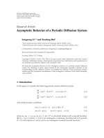
Figure 1: Block diagram representation for the proposed algorithm.
0 50 100 150 200 250 300 350 400 450 500
−30
−25
−20
−15
−10
−5

0
Iterations
EMSE (dB)
α = 0.4 α = 0.6 α = 0.8α = 0.2
Figure 2: Effect of α on the learning curves of the proposed
algorithminanAWGNnoiseenvironmentscenarioforp
= 1.
0 50 100 150 200 250 300 350 400 450 500
−30
−25
−20
−15
−10
−5
0
Iterations
EMSE (dB)
α = 0.4 α = 0.6 α = 0.8α = 0.2
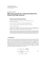
Figure 3: Effect of α on the learning curves of the proposed
algorithm in a Laplacian noise environment scenario for p
= 1.
0 50 100 150 200 250 300 350 400 450 500
−30
−25
−20
−15
−10
−5
0
Iterations

EMSE (dB)
α = 0.4 α = 0.6 α = 0.8α = 0.2
Figure 4: Effect of α on the learning curves of the proposed
algorithm in a uniform noise environment scenario for p
= 1.
0 500 1000 1500 2000 2500 3000 3500 4000 4500
5000
−25
−20
−15
−10
−5
0
Iterations
EMSE (dB)
Laplacian Gaussian Uniform
Figure 5: Learning curves of the proposed algorithm in different
noise environments scenarios for α
= 0.2andSNRof0dB.
a white Gaussian noise, Laplacian noise, and uniform noise,
respectively, for the case of p
= 1. As can be depicted from
thesefiguresthebestperformanceisobtainedwhenα
= 0.8.
More importantly, the best noise statistics for this scenario
is when the noise is Laplacian distributed. An enhancement
in performance is obtained, and about a 2 dB improvement
is achieved for all values of α. Also, one can notice that the
worst performance is obtained when the noise is uniformly
distributed.

Figures 5, 6, 7, 8, 9 and 10 report the performance of the
proposed algorithm for an SNR of 0 dB, 10 dB and 20 dB,
respectively, for the case of p
= 4. Figures 5 and 6 are
the result of the simulations for α
= 0.2andα = 0.8,
respectively. A consistency in performance of the proposed
algorithm in these scenarios f or the uniform noise as far
as the lowest EMSE is reached by the proposed algorithm.
8 EURASIP Journal on Advances in Signal Processing
0 500 1000 1500 2000 2500 3000 3500 4000 4500
5000
Iterations
EMSE (dB)
Laplacian Gaussian Uniform
−30
−25
−20
−15
−10
−5
0
5
Figure 6: Learning curves of the proposed algorithm in different
noise environments scenarios for α
= 0.8andSNRof0dB.
0 500 1000 1500 2000 2500 3000 3500 4000 4500
5000
Iterations
EMSE (dB)

Laplacian Gaussian Uniform
−35
−30
−25
−20
−15
−10
−5
0
Figure 7: Learning curves of the proposed algorithm in different
noise environments scenarios for α
= 0.2andSNRof10dB.
0 500 1000 1500 2000 2500 3000 3500 4000 4500
5000
Iterations
EMSE (dB)
Laplacian Gaussian Uniform
−35
−30
−25
−20
−15
−10
−5
0
Figure 8: Learning curves of the proposed algorithm in different
noise environments scenarios for α
= 0.8andSNRof10dB.
−50
−45

−40
−35
−30
−25
−20
−15
−10
−5
0
0 500 1000 1500 2000 2500 3000 3500 4000 4500
5000
Iterations
EMSE (dB)
Laplacian Gaussian Uniform
Figure 9: Learning curves of the proposed algorithm in different
noise environments scenarios for α
= 0.2andSNRof20dB.
−45
−40
−35
−30
−25
−20
−15
−10
−5
0
0 500 1000 1500 2000 2500 3000 3500 4000 4500 5000
Iterations
EMSE (dB)

Laplacian
Gaussian Uniform
Figure 10: Learning curves of the proposed algorithm in different
noise environments scenarios for α
= 0.8andSNRof20dB.
Similar behaviour is obtained by the proposed algorithm in
Figures 7 and 8 where Figures 7 and 8 report the simulations
results of the proposed algorithm for α
= 0.2andα = 0.8,
respectively, for an SNR of 10 dB.
InthecaseofanSNRof20dB,Figures9 and 10 depict
the results. The case of α
= 0.2isshowninFigure9 while
that of α
= 0 .8isshowninFigure10.Onecanseethat,even
though the proposed algorithm is still performing better in
the uniform noise environment, as shown in Figure 9,for
α
= 0.2, however, identical performance is obtained by the
different noise environments when α
= 0.8asreportedin
EURASIP Journal on Advances in Sig nal Processing 9
Table 1: Theoretical and s imulation EMSE for p = 4, α = 0.2.
Gaussian Laplacian Uniform
Theoretical Simulation Theoretical Simulation Theoretical Simulation
0dB −16.9 −16.85 −9.62 −9.82 −22.81 −22.6
10 dB
−26.02 −26.53 −19.33 −19.99 −31.64 −31.29
20 dB
−44.14 −43.93 −40.34 −40.55 −45.14 −45.43

Table 2: Theoretical and s imulation EMSE for p = 4, α = 0.8.
Gaussian Laplacian Uniform
Theoretical Simulation Theoretical Simulation Theoretical Simulation
0dB −22.47 −22.6 −14.26 −16.02 −27.65 −26.59
10 dB
−28.7 −28.64 −26.41 −26.32 −29.15 −29.57
20 dB
−39.28 −39.87 −39.24 −39.58 −39.28 −39.92
0 1000 2000 3000 4000 5000 6000 7000 8000 9000 10000
−35
−30
−25
−20
−15
−10
−5
0
Iterations
EMSE (dB)
Laplacian Gaussian Uniform
Figure 11: Learning behavior of the proposed algorithm in the
different noise environments scenarios for p
= 4andα = 0.2.
Figure 10. The theoretical findings confirm these results as
will be seen later.
From the above results, one can conclude that when
α
= 0.2 the proposed algorithm is biased towards the LMF
algorithm, in contrast to the case when α
= 0.8, the proposed

algorithm is biased towards the LMS algorithm.
Ne xt, to assess further the performance of the proposed
algorithm for the same steady-state value, two different cases
for α are considered, that is, α
= 0.2andα = 0.8. Figures
11 and 12 illustrate the learning behavior of the proposed
algorithm for α
= 0.2andα = 0.8, respectively, both
are for p
= 4. As can be seen from these figures that the
best p erformance i s obtained with uniform noise while the
worst performanc e is obtained with Laplacian. The mixing
variable α had little effect on the speed of convergence of
the proposed algor ithm when the noise is uniformly and
Gaussian distributed. Ho wever, as can be seen from Figure 12
in the case of Laplacian noise, α
= 0.8hasdecreasedthe
speed of convergence of the proposed algorithm from 55000
iterations (in the case of α
= 0.2) to almost 2000 iterations.
−35
−30
−25
−20
−15
−10
−5
0
Iterations
EMSE (dB)

Laplacian Gaussian Uniform
0 500 1000 1500 2000 2500 3000 3500 4000
Figure 12: Learning behavior of the proposed algorithm in the
different noise environments scenarios for p
= 4andα = 0.8.
A gain of 3500 iterations in favor of the proposed algorithm
when the noise is Laplacian distributed.
Finally, the analytical results for the steady-state EMSE
derived for the proposed algorithm given in (66)arecom-
pared with the ones obtained from simulation for Gaussian,
Laplacian, and uniform noise environments with an SNR
of 0 dB, 10 dB, and 20 dB. This comparison is reported in
Tab l e s 1-2, and as can be seen from these tables, a close
agreement exists between theory and the simulation results
as mentioned earlier, for the case of p
= 4andα = 0.8, that
similar performance by the d ifferent noise environments is
obtained for and SNR of 20 dB as shown in Table 2.
6. Conclusion
A new adaptive scheme for system identification has been
introduced, where a controlling parameter in the range
[0, 1] is used to control the mixture of the two norms. The
derivation of the algorithm is worked out, and the convexity
property is proved for this algorithm. Existing algorithms,
10 EURASIP Journal on Advances in Signal Processing
for example [16–18] can be considered as a special case of the
proposed algorithm. Also, the first moment behaviour as well
as the second moment behaviour of the weights are studied.
Bounds for the step size on the convergence of the proposed
algorithm are derived. Finally, the steady-state analysis was

carried out; simulation results performed for t he purpose of
validating theory are found to be in good agreement with the
theory developed.
The proposed algorithm has been applied so far to a
system identification scenario, for example, echo cancella-
tion. As a future extension, recent work is going on the
application of the proposed algorithm to mitigate the effects
of intersymbol interference in a communication system.
Acknowledgment
The author would like to acknowledge the support of King
Fahd University of Petroleum and Minerals to carry out this
research.
References
[1] B. Widrow and S. D. Stearns, Adaptive Signal Processing,
Prentice-Hall, Englewood Cliffs, NJ, USA, 1985.
[2] S. Sherman, “Non-mean-square error criteria,” IRE Transac-
tions on Information Theory, vol. 4, no. 3, pp. 125–126, 1958.
[3] J. I. Nagumo and A. Noda, “A learning m ethod for sys-
tem identification,” IEEE Transactions on Automatic Control,
vol. 12, pp. 282–287, 1967.
[4] T. A. C. M. Claasen and W. F. G. M ecklenbraeuker , “Com-
parisons of the convergence of two algorithms for adaptive
FIR digital filters,” IEEE Transactions on Circuits and Systems,
vol. 28, no. 6, pp. 510–518, 1981.
[5] A. Gersho, “Adaptive filtering with binary reinforcement,”
IEEE Transactions on Information Theory,vol.30,no.2,
pp. 191–199, 1984.
[6] A. Feuer and E. Wei nstein, “Convergence analysis of LMS
filters with uncorrelated data,” IEEE Transactions on Acoustics,
Speech, and Signal Processing, vol. 33, no. 1, pp. 222–230, 1985.

[7]N.J.Bershad,“Behaviorofthee-normalizedLMSalgorithm
with Gaussian inputs,” IEEE Transactions on Acoustics, Speech,
and Signal Processing, vol. 35, no. 5, pp. 636–644, 1987.
[8] E. Eweda, “Convergence of the sign algorithm for adaptive fil-
tering with correlated data,” IEEE Tr ansactions on Information
Theory, vol. 37, no. 5, pp. 1450–1457, 1991.
[9]S.C.DouglasandT.H.Y.Meng,“Stochasticgradient
adaptation under general error criteria,” IEEE Transactions on
Signal Processing, vol. 42, no. 6, pp. 1335–1351, 1994.
[10] T. Y. Al-Naffouri, A. Zerguine, and M. Bettayeb, “A unifying
view of error nonlinearities in LMS adaptation,” in Proceedings
of the IEEE International Conference on Acoustics, Speech and
Signal Processing (ICASSP ’98), pp. 1697–1700, May 1998.
[11] H. Zhang and Y. Peng, “l
p
-norm based minimisation algo-
rithm for signal parameter estimation,” Electronics Letters,
vol. 35, no. 20, pp. 1704–1705, 1999.
[12] S. Siu and C. F. N. Cowan, “Performance analysis of the lp
norm back propagation algorithm for adaptive equalisation,”
IEE Proceedings, Part F: Radar and Signal Processing, vol. 140,
no. 1, pp. 43–47, 1993.
[13] R. A. Vargas and C. S. Burrus, “The direct design of recursive
or IIR digital filters,” in P roceedings of the 3r d International
Symposium on Communications, Control, and Signal Processing
(ISCCSP ’08), pp. 188–192, March 2008.
[14] S. Haykin, Adaptive Filter Theory, Prentice-Hall, Upper -Saddle
River, NJ, USA, 4th edition, 2002.
[15] E. Walach and B. Widrow, “The least mean fourth (LMF)
adaptive algorithm and its family,” IEEE Transactions on

Information Theory, vol. 30, no. 2, pp. 275–283, 1984.
[16] O. Tanrikulu and J. A. Chambers, “Convergence and steady-
state properties of the least-mean mixed-norm (LMMN)
adaptive algorithm,” IEE Proceedings Vision, Image & Signal
Processing, vol. 143, no. 3, pp. 137–142, 1996.
[17] A. Zerguine, C. F. N. Cowan, and M. Bettayeb, “LMS-LMF
adaptive scheme for echo cancellation,” Electronics Letters,
vol. 32, no. 19, pp. 1776–1778, 1996.
[18] A.Zerguine,C.F.N.Cowan,andM.Bettayeb,“Adaptiveecho
cancellation using least mean mixed-norm algorithm,” IEEE
Transactions on Signal Processing, vol. 45, no. 5, pp. 1340–1343,
1997.
[19] S. Siu, G. J. Gibson, and C. F. N. Cowan, “Decision feedback
equalisation using neural network structures and p erformance
comparison with standard architecture,” IEE Proceedings, Part
I: Communications, Speech and Vision, vol. 137, no. 4, pp. 221–
225, 1990.
[20] R. Price, “A useful theorem for non-linear devices having
Gaussian inputs,” IEEE Transactions on Information Theory,
vol. 4, pp. 69–72, 1958.
[21] J. E. Ma zo, “On the independence theory of equalizer con-
vergence,” The Bell System Technical Journal, vol. 58, no. 5,
pp. 963–993, 1979.
[22] O. Macchi, Adaptive Processing: The Least Mean Squares
Approach with Applications in Transmission,JohnWiley&
Sons, West Sussex, UK, 1995.
[23] A. H. Sayed, Fundamentals of Adaptive Filtering,Wiley-
Interscience, New York, NY, USA, 2003.