Báo cáo hóa học: " Research Article Automatic IP Generation of FFT/IFFT Processors with Word-Length Optimization for MIMO-OFDM Systems" doc

Hindawi Publishing Corporation
EURASIP Journal on Advances in Signal Pr ocessing
Volume 2011, Article ID 136319, 15 pages
doi:10.1155/2011/136319
Research Ar ticle
Automatic IP Generation of FFT/IFFT Processors with
Word-Length Optimization for MIMO-OFDM Systems
Pei-Yun Tsai, Chia-Wei Chen, and Meng-Yuan Huang
Department of Electrical Engineering, National Central University, Jhongli 32001, Taiwan
Correspondence should be addressed to P ei-Yun Tsai,
Received 26 May 2010; Revised 18 October 2010; Accepted 11 November 2010
Academic Editor: Juan A. L
´
opez
Copyright © 2011 Pei-Yun Tsai et al. This is an open access article distributed under the Creative Commons Attribution License,
which permits unrestricted use, distribution, and reproduction in any medium, provided the original work is properly cited.
A systematic approach is presented for automatically generating variable-size FFT/IFFT soft intellectual property (IP) cores
for MIMO-OFDM systems. The finite-precision effect in an FFT processor is first analyzed, and then an effective word-length
searching algorithm is proposed and incorporated in the proposed IP generator. From the comparison, we show that our analysis
of the finite precision effect in FFT is much more accurate than the previous work. With the flexible architecture a nd the effective
word-length searching techniques, we can strike a good balance for the performance and the hardware cost of the generated IP
cores. The generated FFT soft IP cores are portable and independent of the silicon technology, which helps to greatly reduce
the design time. Experimental results demonstrate that the proposed IP generator indeed provides FFT IPs which meet the
requirements and are more suitable in recent MIMO-OFDM communication standards/drafts than some conventional FFT IP
generators.
1. Introduction
Orthogonal frequency-division multiplexing (OFDM) is one
of the most popular modulation schemes in recent wireless
communication systems. In OFDM transceivers, discrete
Fourier transform (DFT) operation plays an important role
to modulate data onto each subcarrier. With the fast Fourier

transform (FFT) algorithm, hardware implementation of
DFT, which is not only computation intensive but also
communication intensive, becomes feasible.
Different OFDM systems use various FFT sizes to accom-
modate time-selective and/or frequency-selective channel
environments. Even in one system, FFT operations of
variable sizes are mandatory to offer the scalability for perfor-
mance considerations. In addition, multiple-input multiple-
output (MIMO) antenna configuration is a widely adopted
technique recently, which needs a multichannel FFT/IFFT
processor in a transmitter/receiver. An extensive literature
exists, which reports the lower-power/small-area/high-speed
implementation of the dedicated FFT processors for cer-
tain single-input single-output (SISO) wireless communi-
cation standards/specifications [1–5] and for multiple-input
multiple-output OFDM systems [6, 7].
However, it is a time-consuming work if a dedicated FFT
processor is redesigned each time for every communication
system. In the past, several general-purpose FFT IP core
generators have also been developed [8–11] including the
state-of-the-art spiral program [12, 13]. On the other hand,
FFT/IFFT core generators specific for OFDM systems can
be seen in [14, 15]. In [11, 12, 15], the generated hardware
employs the radix-2 FFT algorithm and different degrees
of parallelism are exploited, either using multiple butterfly
stages or multiple butterfly units inside a butterfly stage,
to tradeoff throughput requirements and hardware costs.
Radix-2 and radix-4 pipelined multipath delay commutator
architectures have been used in [8, 9]. Higher radix algo-
rithm (radix-2/4/8) was first utilized in [14], which adopts

memory-based architecture and pipelined single-path delay
feedback architecture. Note that the FFT/IFFT core generator
in [15–17] is capable of generating an FFT IP that handles
variable-size FFT/IFFT operations and satisfies the signal-to-
quantization-noise-ratio (SQNR) constraint.
In this paper we propose an IP generator to offer user-
specific FFT processors targeting at the requests in recent and
emerging MIMO-OFDM communication systems. However,
2 EURASIP Journal on Advances in Signal Processing
different from previous works, we try to analyze the finite
precision effect in FFT processors and aim to offer an FFT
IP generator that has the capability of automatic word-
length optimization to achieve hardware efficiency. The IP
generator can generate the hardware description language
of an FFT processor according to the constraints set by
users and therefore speed up the process for implementing
a new OFDM transceiver. Its features can be summarized as
follows.
(i) Parallel processing and multiple channels are taken
into consideration, either to increase throughput or
to support MIMO configurations.
(ii) The word lengths are optimized, which can be shown
to provide more efficient hardware design under the
constraint of SQNR values than some conventional
works [15, 16].
(iii) Insertion of pipeline registers mainly depends on the
requirement of operating frequency to ensure the
necessity of flip-flop instantiation.
From the experimental results, we can see that these
improvements are effective to generate FFT IPs that strike a

good balance between complexity and performance.
The rest of the paper is organized as follows. In Section 2,
the generic FFT architecture adopted by the proposed FFT
IP generator is illustrated. In Section 3,wediscussthefinite
precision effect in FFT operation. The work flow of the IP
generator and the word-length optimization procedure are
delineated in Section 4. Experimental results and compar-
isons are shown in Section 5. Finally, Section 6 gives a brief
conclusion.
2. Architecture of FFT Processors with MIMO
Configuration and Parallel Processing
In Ta ble 1 , we have listed some essential parameters in several
recent OFDM standards/drafts. Note that in UWB using
MB-OFDM modulation scheme, we show its one-channel
sampling rate. It is clear that the needed FFT processor
must support variable sizes as well as parallel processing for
either high throughput or multiple channels. In addition,
the FFT sizes mainly range from 64 points to 8192 points,
and the operating frequency covers from tens to hundreds
of mega Hz. To facilitate automatic generation of the FFT
processors fulfilling the above requirements, we resort to
exploit the mapping of its recursive nature to the pipelined
architecture. However, to accomplish parallel processing
with the high-radix algorithm, we proposed to combine two
well-known p ipelined architectures, namely, the single-path
delay feedback (SDF) architecture and the multipath delay
commutator (MDC) architecture.
Figure 1 shows our adopted architecture that is able to
support the parallelism degree of two or four by utilizing
the property of the multipath delay commutator architecture

in parallel processing. If the parallelism degree of p is
desired, where p
= 2or4,aradix-p MDC stage is
first employed. Thereafter, for the p parallelpaths,we
cascade p-channel N/p-point FFT processors implemented
Radix-2
butterfly
PE6
Commutator
MDC SDF
2-channel
N/2
N/2-point FFT
(a)
Radix-4
butterfly
PE4
Commutator
4-channel
MDC
SDF
3N/4
2N/4
N/4
N/4-point FFT
(b)
Figure 1: (a) Architecture of an FFT processor with parallelism
degree of two. (b) Architecture of an FFT processor with parallelism
degree of four.
by the radix-2/2

2
/2
3
single-path delay feedback architecture.
If parallel processing to enhance the throughput is not
necessary, the generated FFT pr ocessor is reduced to the
conventional SDF architecture.
Tabl e 2 compares the hardware complexity of the pro-
posed architecture and several conventional works with par-
allelism [3, 18–24]. However, those works may be designed
for specific applications such as UWB and may have special
optimization at certain stages. Here, we simply consider their
extensions to an N-point FFT processor. Note that hardware
complexity and architecture flexibility are essential concerns.
In our adopted architecture of parallelism degree of two,
one complex multiplier is required in the first radix-2 MDC
processing element and 2(log
8
(N/2)−1) complex multipliers
are used in the remaining two sets of radix-2
3
N/2-point
SDF architecture. Similarly, if the parallelism degree is four,
3 + 4(log
8
(N/4) − 1) complex multipliers are needed in our
architecture instead of 3(log
4
N − 1) complex multipliers in
the conventional radix-4 MD C architecture. Although the

higher radix-2
4
architecture [20, 23]caneffectively reduce
the number of complex multipliers, the constant multipliers
increase. Special scheduling for some specific FFT size can
help to decrease the complexity of the constant multipliers
[19]. Nevertheless it is not easily provided in an IP generator
offering diverse user-specific parameters. Also the folding
scheme (SDF-kR) is not appropriate because higher and
EURASIP Journal on Advances in Sig nal Processing 3
Table 1: FFT parameters in several OFDM systems
FFT size Sampling rate (MHz) MIMO channels
DVB-T/H 2048–8192 9 —
802.11a 64 20 —
802.11n 64–128 40 Up to 4
UWB (MB-OFDM) 128 528 2
802.16e (OFDM) 256 32.7 —
802.16e (OFDMA) 128–2048 20 Up to 4
3GPP-LTE 128–2048 30.7 Up to 4
802.20 512–2048 20 Up to 4
Table 2: Complexity comparison of several FFT processors with parallelism.
Parallelism Architecture Complex m ultipliers Constant multipliers Storages Clock rate Throughput
2Radix-2MDClog
2
N − 1—
3N
2
− 2R 2R
2Radix-2
2

MDF [18]log
2
N − 2—N − 2R 2R
2Radix-2
4
MDF [19, 20]
1
2
log
2
N − 22log
2
N
3N
2
− 2R 2R
2Thiswork
2
3
log
2
N −
5
3
2
3
log
2

N

2

3N
2
− 2R 2R
1Radix-2
3
SDF-4R [21]
1
3
log
2
N − 1
1
3
log
2
N 4(N − 1) 4R 4R
4Radix-4MDC
3
2
log
2
N − 3—
5N
2
− 4R 4R
4Radix-2
3
MDF [3]

4
3
log
2
N − 4
4
3
log
2
N
5N
2
− 4R 4R
4Radix-2
· 4 ·2MDC[22]log
2
N − 4
9
4
log
2
N
5N
2
− 4R 4R
4Radix-2
4
MDF [23]log
2
N − 44log

2
N
5N
2
− 4R 4R
4Thiswork
4
3
log
2
N −
11
3
4
3
log
2
N −
2
3
5N
2
− 4R 4R
higher sampling frequency is used in advanced systems.
With our proposed architecture, the advantage is twofold.
On one hand, the same control flow as the one needed
for generation of multiple-channel FFT processors can be
shared. On the other hand, we still exploit the radix-2
3
algorithm in hardware reduction. From the table, it is clear

that our architecture is flexible and hardware efficient.
Basic arithmetic processing elements (PEs) are shown in
Figure 2 for constructing various FFT processors. While PE1,
PE2, and PE3 are used in the SDF architecture, PE4, PE5,
and PE6 are instantiated in case parallel processing is needed.
PE3 and PE6 compute the radix-2 butterfly operation. PE1
and PE4 handle the extra complex multiplication of
−j.PE2
and PE5 deal with the trivial multiplications of W
1
8
as well
as W
3
8
by shifters and adders. PE4 and PE5 are only utilized
when the deg ree of par allelism is four. The delay buffer with a
size greater than 16 is made up of a memory array addressing
by an incrementer whose current value and previous value
are adopted as the read and write addresses to guarantee the
read operation done before the write operation at the same
address.
The variable FFT sizes are achieved by the alternative data
paths controlled by the multiplexers as shown in Figure 3,
which is an example of 64-point to 4096-point variable-size
single-channel FFT processor. For N
= 2
K
, there are total
K stages. To perform the 2

3n
-point FFT operation, where
3n
≤ K, the signal directly enters the PE1 at the (K −3n+1)th
stage. When 2
· 2
3n
-point FFT is desired, the signal feeds
directly to PE3 at stage ( K
− 3n). If (2
2
· 2
3n
)-point FFT is
executed, we will route the signal going through PE1 at stage
(K
−3(n + 1) + 1), bypassing the next PE2 and entering into
PE3 and its successive stages. Meanwhile, the delay buffer of
4 EURASIP Journal on Advances in Signal Processing
MUXMUX
MUXMUX
MUX
MUXMUX
MUX
MUXMUX
Delay buffer Delay buffer Delay buffer
1
− j
− j
− j

− j
PE1 PE2
PE3
W
1
8
W
1
8
W
3
8
W
3
8
−
−
−
−
−
+
+
+
+
+
+
+
+
+
+

1
PE4
PE5
PE6
S & A
−−
−
−
−
+
+
+
+
−
−
Figure 2: Block diagram of basic arithmetic processing elements.
2048 1024 512
PE1
PE2 PE3
PE1
PE2 PE3
PE1
PE2 PE3
PE1
PE2 PE3
MUL1
MUX1
Stage 1 Stage 2 Stage 3
Stage 4
Stage 5

Stage 6
Stage 7
Stage 8
Stage 9
Stage 10
Stage 11 Stage 12
ROM
ROM
ROM
256 128 64
MUL2
MUL3
MUX3
MUX2
32 16 8
MUX4
42 1
Figure 3: Architecture of the generated SISO variable-length radix-2
3
FFT processor.
PE1 will be programmed to use only one half of its original
size,whichcanbedonebysimplyusingthearithmeticshift
of the counter output to the l eft by 1 bit without changing
the memory array. The gray vertical lines along the data path
denotethepossiblepipeline-register insertion positions. If
the required operating frequency is not high, then according
to the information in the timing library, only parts of these
pipeline registers are instantiated. On the contrary, all of
them will exist if the clock frequency needs to be raised to
over 100 MHz.

As to automatic generation of multichannel FFT IP, it
basically can be regarded as constructing a two-dimensional
PE array. The number of columns in the PE array relates
to the number of stages. On the other hand, the number
EURASIP Journal on Advances in Sig nal Processing 5
PE1 PE1PE2 PE3
PE1 PE2 PE3
PE1 PE2 PE3
PE1 PE2 PE3
32 16 8
32 16 8
32 16 8
32 16 8
4
PE1
4
PE1
4
PE1
4
Stage K-3
Stage K-2
Stage K-1 & K
PE5
Commutator
Commutator
Modified constant multiplier
ROM
···
···

···
···
Figure 4: Architecture of a MIMO FFT processor with 4 channels.
Q
Q
Q
Q
Q
Q
Q
Q
Q
Q
Q
Q
Q
Q
Q
Q
Q
Q
Q
Q
Q
Q
Q
Q
Q
Q
Q

Q
Q
Q
Q
Q
Q
Q
Q
Q
Q
Q
Q
Q
Radix-4
Radix-2
W
0n
N
W
4n
N
W
2n
N
W
6n
N
W
1n
N

W
5n
N
W
3n
N
W
7n
N
y
p
(n)
x
s−1
(n)
x
s−1
(m)
x
s
(n)
− j
− j
− j
W
1
8
W
3
8

−
−
−
−
−
−
−
−
−
−
−
−
σ
2
PE,s
−1
σ
2
PE,s
σ
2
CM,p
Figure 5: Signal flow graph of the radix-2
3
algorithm.
of rows corresponds to the number of channels. However,
if we simply duplicate the single-channel FFT processor
several times to obtain a multichannel FFT processor, the
hardware redundancy exists. Therefore, the hardware sharing
techniques are employed in the generated IP core. Generally,

in M-channel FFT processors, because independent M data
streams are processed simultaneously, only one ROM table
will be generated and its output is connected to M twiddle-
factor multipliers. The ROM table saves only twiddle factors
in [0, π/4], and we use the symmetry of sine/cosine wave-
forms to derive the values of the remaining twiddle factors.
In the special case of a four-channel FFT processor in MIMO
systems, a modified constant multiplication module and PE5
are adopted to save hardware complexity in the tail stages as
shown in Figure 4 [3]. The modified constant multiplication
module contains eight sets of shifters and adders for the
twiddle factors W
n
64
, n = 1, 2, , 8, which can have 38%
complexity reduction compared to four complex multipliers
according to [3 ]. An extra commutator is required to reorder
the four-channel signals so that different sets of shifters and
adders can be used by the four data paths without conflict.
As a result, for 4-channel FFT handling more than 64 points,
architecture in Figure 4 is employed. If an FFT processor
dealing with more than 256 points with parallelism level of 4
is required, architectures of Figures 1 and 4 will be combined
and generated.
By adopting the radix-2
3
algorithm and the flexible
architecture that utilizes both SDF and MD C, t he proposed
IP generator thus supports multichannel as well as parallel
processing, one fixed-size or multiple variable-size, and user-

specified operating frequency with reduced complexity.
3. Finite Precision Effect and
Word-Length Optimization
To design a proper word-length searching procedure, we
need to realize the mean squared quantization error due
to the finite precision effect. Observe the signal flow graph
of the radix-2
3
FFT operation as given in Figure 5.Itis
clear that only two types of arithmetic computations are
involved, that is, complex addition/subtraction and complex
multiplication. In addition, the twiddle factors are all pure
fractional numbers except for
±1 and 0. Obviously they cause
a long word length in the fractional part after multiplication.
Hence, to avoid rapid growth in hardware complexity, trun-
cation is ne cessary. In Figure 5,thecirclewith“Q” denotes
the introduction of the probable quantization effect due to
truncation. In the following, the mean squared quantization
errors resulted from these two types of arithmetic operations
and the truncation are analyzed. Note that these analyses are
also applicable to radix-2 and radix-4 algorithms.
3.1. Quantization Error after Complex Addition/Subtraction.
Assume that two input signals to be summed are denoted as
6 EURASIP Journal on Advances in Signal Processing
x
s
(n)aswellasx
s
(m), where x

s
(n)isthenth signal at the
sth stage, the notation (
·) indicates the quantized version
of the signal, and m
= n + N/2
s
. The output after complex
addition/subtraction is given by
x
s+1
(
n
)
=

x
r,s+1
(
n
)
+ j
x
i,s+1
(
n
)
=

x

r,s+1
(
n
)
+ δ
r,s+1
(
n
)

+ j

x
i,s+1
(
n
)
+ δ
i,s+1
(
n
)

=

x
r,s
(
n
)

+ x
r,s
(
m
)
+ δ
r,s
(
n
)
+ δ
r,s
(
m
)

+ j

x
i,s
(
n
)
+ x
i,s
(
m
)
+ δ
i,s

(
n
)
+ δ
i,s
(
m
)

,
x
s+1
(
m
)
=

x
r,s
(
n
)
− x
r,s
(
m
)
+ δ
r,s
(

n
)
− δ
r,s
(
m
)

+ j

x
i,s
(
n
)
− x
i,s
(
m
)
+ δ
i,s
(
n
)
− δ
i,s
(
m
)


,
(1)
where x
r,s
(n)andx
i,s
(n) denote the real part and imaginary
part of x
s
(n)andδ
r,s
(n)andδ
i,s
(n) represent the real part
and the imaginary part of the quantization error, which may
have nonzero mean. Assume the mean square error at the sth
PE stage due to δ
r,s
(n)andδ
i,s
(n)asσ
2
PE,s
. Note that one half
of the signals at the (s + 1)th stage is computed by addition
while the other half is computed by subtraction. Therefore,
the mean of the quantization error (
x
s+1

(n) − x
s+1
(n)) with
n
= 0, 1, , N − 1atstage(s +1)isgivenby
μ
PE,s+1
= E

δ
r,s
(
n
)

+ jE

δ
i,s
(
n
)

=
μ
PE,s
. (2)
The mean squared quantization error after addition and
subtraction can be calculated respectively as
E






x
r,s+1
(
n
)
− x
r,s+1
(
n
)

+ j


x
i,s+1
(
n
)
− x
i,s+1
(
n
)




2

=
E



δ
r,s
(
n
)
+ δ
r,s
(
m
)


2

+ E



δ
i,s
(

n
)
+ δ
i,s
(
m
)


2

,
E





x
r,s+1
(
m
)
−x
r,s+1
(
m
)

+ j



x
i,s+1
(
m
)
− x
i,s+1
(
m
)



2

=
E



δ
r,s
(
n
)
− δ
r,s
(

m
)


2

+ E



δ
i,s
(
n
)
− δ
i,s
(
m
)


2

.
(3)
With the assumption of uncorrelated quantization errors, the
mean squared error at stage (s + 1) becomes
σ
2

PE,s+1
= 2σ
2
PE,s
. (4)
Details are shown in Appendix A.
3.2. Quantization Error after Complex Multiplication.
Assume that W
r,p
(m)andW
i,p
(m) indicate the real part
and the imaginary part of the mth twiddle factor at the
pth complex multiplication block. The nth quantized signal
y
p
(n)afterthepth complex multiplication takes the form of
y
p
(
n
)
=

y
r,p
(
n
)
+ j

y
i,p
(
n
)
=

x
r,s
(
n
)
+ δ
r,s
(
n
)

+ j

x
i,s
(
n
)
+ δ
i,s
(
n
)


·

W
r,p
(
m
)
+

r,p
(
m
)

+ j

W
i,p
(
m
)
+

i,p
(
m
)

≈


x
r,s
(
n
)
W
r,p
(
m
)
− x
i,s
(
n
)
W
i,p
(
m
)

+

W
r,p
(
m
)
δ

r,s
(
n
)
− W
i,p
(
m
)
δ
i,s
(
n
)

+

x
r,s
(
n
)

r,p
(
m
)
− x
i,s
(

n
)

i,p
(
m
)

+ j

x
r,s
(
n
)
W
i,p
(
m
)
+ x
i,s
(
n
)
W
r,p
(
m
)


+

W
i,p
(
m
)
δ
r,s
(
n
)
+ W
r,p
(
m
)
δ
i,s
(
n
)

+

x
r,s
(
n

)

i,p
(
m
)
+ x
i,s
(
n
)

r,p
(
m
)

,
(5)
where

r,p
(m)and
i,p
(m) denote the real-part and the
imaginary-part quantization errors of the twiddle factor.
Since the twiddle factors can be predetermined by rounding
operation, the y can be assumed to have zero mean. The
statistics of quantization errors after complex multiplication
can be derived as

μ
CM,p
=

E

W
r,p
(
m
)

E

δ
r,s
(
n
)

−
E

W
i,p
(
m
)

E


δ
i,s
(
n
)


+ j

E

W
i,p
(
m
)

E

δ
r,s
(
n
)

+E

W
r,p

(
m
)

E

δ
i,s
(
n
)


,
σ
2
CM,p
≈ E





W
r,p
(
m
)
δ
r,s

(
n
)
− W
i,p
(
m
)
δ
i,s
(
n
)
+x
r,s
(n)
r,p
(m) − x
i,s
(n)
i,p
(m)




2

+ E






W
i,p
(
m
)
δ
r,s
(
n
)
+ W
r,p
(
m
)
δ
i,s
(
n
)
+x
r,s
(
n
)


i,p
(
m
)
+ x
i,s
(
n
)

r,p
(
m
)




2

.
(6)
Similarly, by applying the assumption of uncorrelated errors
of δ
r,s
(n), δ
i,s
(n)
r,p
(m), and 

i,p
(m), and mutually indepen-
dent random variables of the data paths and twiddle factors,
the mean squared error becomes
σ
2
CM,p
≈ E




W
r,p
(
m
)
δ
r,s
(
n
)



2

+ E





W
i,p
(
m
)
δ
i,s
(
n
)



2

+ E




x
r,s
(
n
)

r,p
(

m
)



2

+ E




x
i,s
(
n
)

i,p
(
m
)



2

−
2E





W
r,p
(
m
)
W
i,p
(
m
)
δ
r,s
(
n
)
δ
i,s
(
n
)




+ E





W
i,p
(
m
)
δ
r,s
(
n
)



2

+ E




W
r,p
(
m
)
δ
i,s
(

n
)



2

EURASIP Journal on Advances in Sig nal Processing 7
+ E




x
r,s
(
n
)

i,p
(
m
)



2

+ E





x
i,s
(
n
)

r,p
(
m
)



2

+2E




W
r,p
(
m
)
W
i,p

(
m
)
δ
r,s
(
n
)
δ
i,s
(
n
)




=
2E

W
2
r,p
(
m
)
+ W
2
i,p
(

m
)

σ
2
PE,s
2
+2E

x
2
r,s
(
n
)
+ x
2
i,s
(
n
)

σ
2
T,p
2
,
(7)
where the mean squared error of the twiddle factors at the
pth complex multiplication block, E

{

2
r,p
+ 
2
i,p
}, is denoted
as σ
2
T,p
.
It is clear that i n (7), the term (W
2
r,p
(m)+W
2
i,p
(m)) has
unit magnitude. On the other hand, according to Parseval’s
theorem, we can derive the average of (x
2
r,s
(n)+x
2
i,s
(n)). The
derivations are available in Appendix B.Inourcaseofthe
radix-2 butterfly,
E


x
2
r,s
(
n
)
+ x
2
i,s
(
n
)

=
2
s
N
2
N
−1

k=0
|X
(
k
)
|
2
. (8)

Generally, in OFDM systems, the frequency-domain data
X(k) are selected from some pre-determined constellations
with normalized energ y. Consequently, the averaged energy
of frequency domain signal X(k) can be easily computed.
Thus, from (7)and(8), the mean squared error after complex
multiplication becomes
σ
2
CM,p
≈ σ
2
PE,s
+
2
s
N
2
N
−1

k=0
|X
(
k
)
|
2
σ
2
T,p

= σ
2
PE,s
+
2
s
N
σ
2
T,p
. (9)
3.3. Quantization Error after Truncation. Two t y p es of
signal truncation are discussed here. One is truncation
after multiplication and the other is truncation after
addition/subtraction. Different error distributions can be
observed in each case.
If the fractional parts of the twiddle factor and the data
path contain b
t
and b
d
bits, respectively, then after complex
multiplication, the word-length in the fractional part of the
product becomes b
t
+ b
d
bits. Therefore, truncation is often
performed. As shown in Figure 6,defined
= 2

−(b
t
+b
d
)
as
the finest granularity. After truncation, we use b
m
bits in the
fractional part. Note that D
= 2
−b
m
= 2
M
d,whereM =
b
t
+b
d
−b
m
. Because FFT involves a lot of butterfly operations,
according to the central limit theorem, for d
 D,the
quantization error can be modeled as Gaussian distribution
which may be biased and thus have a nonzero mean α as
indicated in Figure 6. The distance between the floating-
point representation y
r,p

(n) and the nearest fixed-point
representation in the finest granularity is denoted by t.After
truncation, all the signals
y
r,p
(n) inside one of the shadowed
region now are classified as
z
r,p
(n) and have squared error of
(t + id
− lD)
2
,wherel = 0, ±1, ±2, ihas equal probability
ranging from 0 to 2
M
− 1andt is assumed to be uniformly
distributed in [0, d).
Define the conditional probability on t and i of the
quantization error falling in each shadowed region indexed
by l as g(l
| t, i), which can be computed as
g
(
l
| t, i
)
=

−t−id+(l+1)D

−t−id+lD
1
√
2πν
e
−(x+α)
2
/2ν
2
dx
=q

−
t−id+α+lD
ν

−
q

−
t−id+α+
(
l+1
)
D
ν

,
(10)
where

q

y

=

∞
y
1
√
2π
e
−x
2
dx, (11)
and ν
2
is the variance of quantization error in either the
real or the imaginary part after complex multiplication and
before truncation, which can be calculated as (1/2)(σ
2
CM,p
−
μ
2
CM,p
). Denote f
T
(t) as the probability density function of
t and f

T
(t) = 1/d. Then, after truncation of the bits in
the fractional part, the mean squared error of the complex
output becomes
σ
2
T1,p
= 2
∞

l=−∞
2
M
−1

i=0
1
2
M

d
0
g
(
l | t, i
)
f
T
(
t

)(
t + id
− lD
)
2
dt,
(12)
and the mean of quantization error after truncation can be
given by
μ
T1,p
=

1+ j

∞

l=−∞
2
M
−1

i=0
1
2
M

d
0
g

(
l | t, i
)
f
T
(
t
)(
t + id
− lD
)
dt.
(13)
Equations (12)and(13), which can be computed by numeric
approaches, play an important role to analyze the statistics
of quantization errors owing to truncation after complex
multiplications.
For those cases which use one-bit truncation after the
butterfly operation, the assumption of Gaussian distribution
is not suitable because the inequality D
 d is not satisfied.
We then utilize the same assumption of uniform distribution
as in [25]. Thus, one half of the signal remains the same,
and the other half has additional quantization error of d.
The mean of quantization error after LSB truncation can be
calculated as
μ
T2,s
=


1
2
E

δ
r,s
(
n
)

+
1
2
E

δ
r,s
(
n
)
+ d


+ j

1
2
E

δ

i,s
(
n
)

+
1
2
E

δ
i,s
(
n
)
+ d


=
μ
PE,s
+ d
1+j
2
.
(14)
The mean squared error after LSB truncation c an be derived
as
σ
2

T2,s
=
1
2
E

δ
2
r,s
(
n
)

+
1
2
E


δ
r,s
(
n
)
+ d

2

+
1

2
E

δ
2
i,s
(
n
)

+
1
2
E


δ
i,s
(
n
)
+ d

2

=
σ
2
PE,s
+ dE


δ
r,s
(
n
)
+ δ
i,s
(
n
)

+ d
2
.
(15)
8 EURASIP Journal on Advances in Signal Processing
Unlike in [25], we introduce an extra term to account for the
possible nonzero mean after truncation. In the following, we
can see its influence on the accuracy of the analytic mean
square quantization errors.
3.4. Discussion on Word-Length Optimization. According to
the previous analyses for the finite precision effect in an FFT
processor, some observations are summarized below.
(i) In the radix-2
3
single-path delay feedback architec-
ture, the average s ignal energy is increased by 2
according to Parseval’s theorem (see Appendix B),
while the mean squared quantization error also

doubles after butterfly operation as given by (4).
Define a signal-to-quantization error ratio (SQNR)
as
SQNR
= 10 · log
10
E

|
x
s
(
n
)
|
2

σ
2
PE,s
. (16)
Hence, if the signal is not truncated after butterfly
operation, the SQNR remains the same.
(ii) The SQNR decreases after complex multiplication
because of the finite precision of twiddle factors.
The quantization errors in twiddle factors are further
scaled by the average energy of the signal to be
multiplied as indicated in (9). Consequently, the
word-length settings of twiddle factors and data paths
should be decided individually. Moreover, (9), also

reveals the reason that a shorter word-length can
always be assigned for twiddle factors than the data
path in an FFT processor since 2
s
/N  1.
(iii) The mean squared quantization errors increase
monotonically from the first stage to the last stage.
For t hose stages at which quantization errors accu-
mulate and severely pollute the least significant bits
(LSBs) of finite-precision signals, proper truncation
introduces only negligible degradation compared to
σ
2
PE,s
as in (15)ford
2
 σ
2
PE,s
.
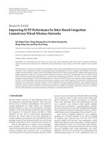
To verify the previous analysis, the analy tic results (12)
and simulated results are compared in Figure 7. The hori-
zontal axis represents the word-length b
m
while the vertical
axis denotes the MSE. Twiddle factor multiplications for 64-
point and 512-point FFT operations are both evaluated. In
both cases, the twiddle factors are quantized to 10 bits in their
fractional part. The fractional part of the input data-path
signal before multiplication is represented by 11 bits and 12

bits in 64-point and 512-point FFT, respectively. Accordingly,
without truncation, the fractional parts become 21 and 22
bits. From the figure, we can see that the analytic results
approach the simulated results. Besides, the proper word-
length b
m
can b e selected around the knee point close to t he
error floor, which implies that only slight degradation occurs.
In Figure 8, the analytic results by using (4), (9), (12),
and (15) and the simulated results of the mean squared
quantization errors at each stage for 512-point FFT are
compared. In addition, we also provide the curve of the
analytic results by [25]. The effect of W
1
8
and W
3
8
in PE2
t
D
d

Z
r,p
(n)
y
r,p
(n)
l

=−1
l = 0
id
α
E
{y
r,p
(n)}
6ν
Figure 6: Quantization error distribution.
8 1012141618
10
−4
10
−5
10
−6
10
−7
10
−8
Fractional part word-length after truncation
MSE
Analytic results (w ith W
m
64
)
Simulated results (with W
m
64

)
Analytic results (w ith W
m
512
)
Simulated results (with W
m
512
)
Figure 7: Analytic and simulated quantization mean squared error
after truncation.
is ignored temporarily. The word lengths of the output
at each stage after truncation are also indicated. It can
be seen that if there is no truncation after the PE stages,
the slope of the segment is log(2)/stage. If a proper word
length around the knee point is chosen after complex
multiplication, a nonzero slope of the segment appears but is
still less than log(2)/stage. On the other hand, if truncation
is performed after complex addition/subtraction, the slope
becomes steep. This figure demonstrates that our analytic
result that considers the bias effect after truncation and uses
Gaussian distribution approximating the quantization error
EURASIP Journal on Advances in Sig nal Processing 9
10
−4
10
−5
10
−6
10

−7
10
−8
Mean squared error
Simulated MSE
Analytic MSE
Analytic MSE [25]
12 bits
12 bits
12 bits
12 bits
10 bits
10 bits
11 bits
truncation after CM
truncation after CM
one-bit truncation
9 bits
11 bits
One-bit truncation
Stage 1
Stage 2
Stage 3
CM 1
Stage 4
Stage 5
Stage 6
CM 2
Stage 7
Stage 8

Stage 9
10-bit
12-bit
Figure 8: Comparison of analytic and simulated mean squared
quantization errors at each stage in a 512-point FFT processor.
Input
parameters
Word-length
optimization
Instantiation &
connection
Output files
Timing
library
Instance
library
Figure 9: Flowchart of the proposed IP generator.
after complex multiplication can estimate the finite precision
effect more accurately.
4. Work Flow
The work flow of the IP generator is indicated in Figure 9.
In the first s tep, a user assigns his options such as the
FFT size, configurations of parallelism, t arget operating
frequency, allowable SQNR, and the FFT/IFFT mode for
his desired IP core. Then, in order to minimize the finite
precision effect, the word-length of each block will be
optimized based on the SQNR c riterion. In the third step,
the IP generator instantiates the related submodules from
the library and connects those submodules in the highest-
hierarchy top module. Finally, together with the desired

hardware description language of the FFT processor, we also
provide the test bench to users. We will describe the details of
these four steps in the following.
4.1. Input Parameters. The proposed IP generator provides
five main options.
4.1.1. FFT or IFFT Mode. In an OFDM system, the IFFT
operation is needed in a transmitter while the FFT operation
should be done in a receiver. The IFFT operation can be
written as
x
(
n
)
=
1
N
N−1

k=0
X
(
k
)
W
−nk
N
=
1
N
⎡

⎣
N−1

k=0
X
∗
(
k
)
W
nk
N
⎤
⎦
∗
, (17)
which can be interpreted as applying the FFT operation to
the complex conjugate of the inputs and then dividing the
complex conjugate of the FFT output by N.SinceN is a
power of two, no extra hardware is required for the division.
Hence, the proposed IP generator can provide the IFFT
processor by incorporating additional paths to derive the 2’s
complement of the imaginary part of both the inputs to the
FFT processor and outputs from the FFT processor.
4.1.2. FFT/IFFT Size. In Tabl e 1, we can see that the current
and emerging OFDM standards mainly use FFT/IFFT sizes
up to 8192. Consequently, our IP generator can provide one
single-size FFT/IFFT processor from 8 to 8192 points by
cascading adequate processing elements and also produce a
variable-size FFT/IFFT processor in the range of 64 to 4096

points by adding multiplexers to control the data paths.
4.1.3. Sampling Rate. The generated FFT/IFFT processor
must fulfill the system requirement of real-time operation.
The proposed IP generator automatically inserts the neces-
sary pipeline registers in the positions as indicated by the gray
vertical lines in Figure 3 to reduce the critical path delay and
thus satisfies the target of working frequency. In the timing
library, we have constructed a table listing the critical path
delay of PEs and multipliers. The highest frequency around
140 MHz is obtained in 90-nm FPGA, when the critical path
contains only a complex multiplier.
4.1.4. SQNR Value. The finite-word-length representation of
the FFT/IFFT processor inevitably introduces quantization
errors, which degrade system performance. Therefore, the
word lengths of the generated FFT/IFFT IP core must be
optimized according to the requested SQNR value.
4.1.5. Multiple-Channel and Parallel Processing. The gener-
ated processor can support up to eig ht-channel FFT/IFFT
operations to cover the needs in MIMO-OFDM systems.
In addition, parallelism degrees of two or four to enhance
throughputs are also implemented to support wide-band
applications such as UWB.
4.2. Word-Length Optimization. Consider the hardware
complexity related with the word-length settings. The
10 EURASIP Journal on Advances in Signal Processing
Table 3: One example of the proposed fractional-part word-length search procedure.
2
1
Analytic
SQNR

Simulated
SQNR
Tw i ddleStage 8Stage 7Stage 6CMul 2Stage 5Stage 4Stage 3CMul 1Stage 2
56.3556.72912131313131313131313
56.2256.53912121313131313131313
55.9856.23912121213131313131313
55.1055.48912121212121313131313
54.4854.64912121212121213131313
54.7255.04911121212121313131313
54.3854.50911111212
121313131313
46.5147.061111111111111111111111
52.5353.071212121212121212121212
58.5559.081313131313131313131313
58.5159.031213131313131313131313
58.3858.911113131313131313131313
58.0358.521013131313131313131313
56.4956.86913131313131313131313
53.4353.58813
131313131313131313
Stage 1
Search
phase
smaller word length in processing elements, the less com-
plexity the complex adder/subtractor and the delay buffer. If
a smaller word length is assigned to twiddle factors, the size
of ROM tables can be scaled down linearly and the size of the
complex multiplier can also be reduced, which saves more
in silicon cost. The proposed IP generator can automatically
search for the optimal word-length setting of each stage,

which is a feature that the conventional IP generators do not
provide.
Exhaustive search for optimal word lengths is a time-
consuming work. Observing the pipeline architecture, if the
data-path at earlier stages uses a smaller word length, the
delay elements can save more and a smaller-size complex
multiplier is probably instantiated. Hence, we proposed a
procedure which includes two search phases, that is, global
search and local search, which aim to use smaller word-
length settings at the earlier stages. Initially, the same word
length of the fractional part is set at all the PE stages. In
the first p hase, that is, the global search, the fractional-part
word lengths of all the PE stages are increased or decreased
together until an S QNR value of the FFT output closest to
but greater than the target value is obtained. Subsequently,
the reduction of the twiddle-factor word length is not ceased
until the SQNR value is below the target value. In fact, the
global search phase only determines the finest precision of
data paths and twiddle factors, which has also been proposed
in [16]. On the other hand, it has been pointed out in [25]
that using varying word lengths at each stage is viable when
the request of the IP that is optimized for each specific
application is eager. We then proposed a second phase to
finetunethewordlengthateachstage.Thequantization
error accumulates and thus t he LSBs may be contaminated
by quantization errors. We then truncate the LSB from t he
last stage to examine if the target SQNR can be still fulfilled.
If the answer is true, then the test of LSB truncation proceeds
to the earlier stages sequentially until the SQNR value is not
satisfied.Whenithappens,wethenrestorethetruncationat

that stage and initiate a new iteration of LSB truncation from
the last stage again. The procedure goes on so that the word
length at each stage can be minimized.
Tabl e 3 gives the results of word-length optimization
procedure in the global search phase and the local search
phase for 256-point FFT with an SQNR requirement of
55dB. As mentioned earlier, in the global search phase,
one fractional part word length of all the PEs and one
fractional-part word length of all the twiddle factors are
chosen, respectively. We can see that if the LSB at stage
4 is eliminated, the SQNR value becomes unsatisfying.
EURASIP Journal on Advances in Signal Processing 11
Stage Stage Stage
Word length of Mantissa
Exponent
Convergent block floating point
& block floating point
Fixed point
Word length of fixed point
Proposed scheme
Word length of
proposed scheme
(a)
7 8 9 10 11 12 13 14
10
20
30
40
50
60

70
Word-length
This work
Convergent block floating point [16]
Block floating point [16]
Fixed-point [15]
SQNR (dB)
(b)
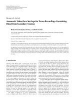
Figure 10: (a) Illustration of different data-path representations and (b) comparison of SQNR values versus word-length settings by different
representations.
Therefore, we can only remove one LSB from stage 5 to stage
8 in the first iteration. Subsequently, the second iteration
starts to truncate one LSB again from the last stage. This time,
one LSB is removed only at stage 8.
In Figure 10(a), we illustrate the word-length assignment
of different representations at each stage, and in Figure 10(b),
the SQNR values versus word lengths under different
representations are given, where the word length of twiddle
factor is set to 18 bits to get rid of its influence and the FFT
size is 2048 points. The block-floating point representation
uses an exponent at each stage to absorb the variation of
dynamic ranges [16]. The convergent block-floating point
representation has several scaling factors at one stage and one
for each group [26]. It converges to one exponent for one FFT
output. The fixed-point representation has only one format
for all the stages, and thus it must take into consideration
both the dynamic range and the precision simultaneously
[15]. The effective range of each representation is i ndicated
by the gray colors in Figure 10(a). With the block-floating
point and convergent block-floating point representations,

we can effectively use the entire dynamic r ange and thus
definitely better performance can be achieved than the pro-
cessor with the fixed-point representation, which may cause
a waste in dynamic range at the early stages. However, in
the conventional word-length searching algorithms for fixed-
point [15] and block-floating point [16] repr esentations,
1 bit increase/decrease in the word length results in 6-dB
change in SQNR. As a result, the processor must choose
the word-length setting that produces SQNR value greater
than the target value. With the proposed algorithm, we
12 EURASIP Journal on Advances in Signal Processing
can approach the desired SQNR value by removing those
harmless LSBs at the last stages compared to the fixed-point
representation as shown in Figure 10(a) and can employ
more flexible and adequate word lengths at each stage.
Since the word lengths at each stage may be different, we
depict the averaged word length of the proposed scheme in
Figure 10(b). It is thus clear that our proposed word-length
algorithm can meet the requirement of any user-specified
SQNR value with reduced silicon cost.
4.3. Instantiation and Connection. Since the architecture to
be generated is very regular, in the library we have prepared
the basic submodules such as PE1 to PE6, a complex
multiplier, a memory array, shift registers, pipeline registers,
a commutator, and multiplexers. After the optimal word-
lengths are derived, we can instantiate related submodules in
the top module.
Nested FOR loops are used in the program to do the
instantiation. In the outer loop, the program will judge
which processing elements should be inserted, whether a

multiplexer is required or not to control the signal flow,
and whether a pipeline register should be included at the
current stage. The look-up t ables for tw iddle factors will
be automatically generated after its word length and the
table size is determined. For the multichannel configuration,
the second inner loop is used to duplicate the submodules
that can not be shared. Once the instantiations of all the
submodules are complete, the wires that connect these
input and output ports are declared and constructed. Sign
extension and LSB truncation are performed necessarily
to ensure correct signal propagation between stages with
different representation formats.
4.4. File Output and Test Bench. Finally, our IP generator will
provide the user an FFT processor IP core and one test bench
to facilitate its verification. For a variable-size FFT processor,
the multiple test benches are offered to verify the correctness
of each respective size.
5. Experimental Results and Comparisons
To verify the proposed IP generator, design examples of
different configurations are tested as shown in Ta b le 4.First,
we use the IP generator to g enerate FFT IP cores. Their
function has been examined to be correct with the auto-
matically generated test b ench. The desired SQNR as well as
the resulted SQNR that adopts the simulated values in the
search procedure is also available in the table. In Table 4(a),
the performance and complexity of the FFT IP cores that
are implemented by FPGA of device xc4vsx55-12 are g iven.
The hardware complexity is evaluated in terms of FPGA
resources of all design examples. The number of flip-flops
is related with the pipeline registers and short d elay buffers,

while the number of slices reflects the logic complexity
including distributed RAMs for long delay buffers and ROMs
for twiddle-factor lookup tables. The DSP slices correspond
to the multipliers. In our generated IP core, the DSP slices
divided by four is exactly the number of complex multipliers.
For applications in UWB systems with a sampling rate
of 528 MHz and a throughput requirement more than 410
Mega samples, four parallel processing blocks are used so that
the operating frequency can be reduced by a factor of 4 [3,
24]. The throughput is calculated by the maximum operating
frequency derived after synthesis. It is clear that the generated
FFT IP meets the requirements of the UWB systems. For
two-channel FFT processors, the complexity grows almost
linearly. In addition, we can see the advantages of the
modified constant multipliers in Figure 4 by comparing the
implementation results of 802.11n with one channel and four
channels.WecanseethattheDSPslicesarereducedfrom
8
× 4 to 16, a 50% reduction in complex multipliers. And
the number of slice grows due to the complexity of shifters
and adders in constant multipliers. As to the large-size FFT
processorsfor3GPP-LTEorDVB-T,theadvantageofthe
radix-2
3
algorithm is clear in that it results in small increase
of the number of complex multipliers. However, in these FFT
processors, large ROM tables with 256 entries in 2048-point
FFT and w ith 1024 entries in 8192-point FFT are required.
Also, the long delay buffers implemented by distributed
RAMs are also entailed. Both occupy large resources of the

number of slices. Although block RAMs in FPGA can be used
instead, owing to that the RAM macro is vendor specific,
we still use the memory array, thus being implemented
by distributed RAMs, to support the applications of the
generated IP cores in cell-base design flow. On the right-
hand side of the table, we compare the IPs generated
by different generators. Due to the fact that the pipeline
registers are not inserted arbitrarily, equal throughput of the
generated FFT processors is not straightforward to come by.
However, we can normalize the hardware complexity to the
throughput and evaluate the relative complexity as the ratio
indicated in the parenthesis. With the radix-2
3
algorithm
and the flexible architecture, our generated IP core uses
less flip-flops and DSP slices (complex multipliers) with a
slightly increased number of slices compared to the ones
generated by Xilinx Logicore and the Spiral program. Thus,
the hardwar e efficiency is better.
In Ta ble 4 (b), the synthesis results of several generated
FFT IP cores by D esign Compiler in 90 nm UMC CMOS
technology are listed. The maximum frequency is derived by
the critical path delay of typical cell library under 1-V supply
voltage. Since the word length at each stage varies in our
works, the average word length of all the butterfly stages is
shown. To get further insight into their logic components,
we indicate the equivalent gate counts of combinational
logic and noncombinational logic. The normalized area is
provided for fair comparison. The original area in their
respective CMOS technology is also given in the parenthesis.

The throughput is derived based on the maximum operating
clock frequency. The power consumption is estimated from
the synthesized results at 1-V supply voltage. Usually it is
pessimistic compared to the measurement results. Other
designs of 64-point FFT processors for 802.11a, 256-point
FFT processors for 802.16e, and an 8-channel FFT processor
are also included. Because the timing information of t he
generatorismainlyderivedthroughtheresultsinVirtex-4
FPGA, for the cell-based design flow, we push the maximum
EURASIP Journal on Advances in Signal Processing 13
Table 4: Experimental results and comparisons of various generated FFT/IFFT processors implemented (a) by FPGA and (b) by cell-base
design flow .
(a)
This work
Spiral [27]
Logicore [10]
(sic)
Standard UWB UWB 802.11n 802.11n
802.16e/3GPP-
LTE
DVB
802.16e
(OFDM)
——
Length 128 128 64∼128 64∼128 128∼2048 2048∼8192 256 256 256
Desired SQNR
(dB)
45 45 55 55 50 45 50 Data: 16 bits Data: 16 bits
Resulted SQNR
(dB)

45.05 45.01 55.65 55.34 50.04 45.01 50.04 — —
MIMO
configurations
12412 1211
Parallel
processing blocks
44111 1141
Target Freq.
(MHz)
410/4 410/4 40 40 32 20 100 — —
Max Freq. (MHz) 152 151 65 45.77 42 22.93 127 198 315
Number of slice
Flip-flops
1829 3628 1753 399 1654 3231 1378 (100%) 2523 (257%) 5198 (304%)
Number of slices 2459 4803 7549 1312 10004 17158 2820 (100%) 1886 (94%) 3370 (96%)
DSP s lices 28 56 16 8 24 16 16 (100%) 16 (140%) 70 (353%)
Throughput
(MSample)
608 604
× 265× 446 42× 2 22.94 127 × 2 181 315
(b)
Ours
[15][2][8]Ours [15][28]
Ours
UWB
Ours [7]
Process (μm) 0.09 0.09 0.35 0.25 0.35 0.09 0.35 0.13 0.09 0.09 0.09
Length 64 64 64 64 64 64
∼256 256 16,64,256 128 256 256
Word length (Bits) 14.8 14.8 13 16 24 14.1 14 16 14.1 12 10

MIMO 4 1 1 1 1 1 1 1 1 8 8
Parallelism 1 1 1 1 1 1 1 1 4 1 1
Max Freq. (MHz) 413 394 60 26 100 417 80 100 407 300 447
Combinational
gate count
78.1 K 19.5 K — — — 35.5 K — — 61.8 K 198.9 K —
Noncombinational
gate count
52.1 K 13.2 K — — — 44.3 K — — 23.7 K 316.6 K —
Total gate count 130.3 K 32.7 K — 61.5 K 105 K 79.8K — 195 K 85.5K 515.5 K 583K
Normalized Area
(mm
2
)
0.408 0.102
0.293
(4.44)
— — 0.250
0.544
(8.228)
— 0.268 0.268 —
Throughput
(MS/s)
413
× 4 394 26.8 72 49 417 33 2 77.1 1628 300 × 8 300 × 8
Power (mW)
147 @
413 MHz
36 @
394 MHz

———
76 @
417 Mz
——
116 @
407 MHz
407 @
300 MHz
160.5
∗
@300 MHz
∗
measurement.
operating clock frequency of our works to the limit. As to
the 256-point FFT processor, we can see that the ratio of
noncombinational logic gates to total gates increases due to
the delay elements, whose quantity is proportional to the FFT
size. With the parallel processing architecture, we can sup-
port FFT processors for Giga samples per second in advanced
communication syste ms. For all the cases, our IP generator
can generate FFT processors with agg ressive throughput and
efficient hardware compared to other generators. From the
table, it is shown that this IP generator is more competitive
to generate FFT processors for various OFDM systems than
previous works.
Although we do not address issues for power reduction,
such as dynamic voltage and frequency scaling in [7]and
thus the power consumption seems larger, the system-level
power saving techniques can still be applied to obtain a
14 EURASIP Journal on Advances in Signal Processing

low-power FFT IP by appropriate parameter settings. For
example, we can set higher operating clock frequency than
the nominal system sampling frequency to generate the
IP that has short critical path delay and then scale down
the supply voltage or synthesize it with a low-speed low-
leakage library [29]. However, there are also some limitations
that the proposed IP generator can not fully replace the
manually designed application-specific IC (ASIC), like the
use of sleep transistors or multiple-threshold transistors,
especially in nanotechnology. Besides, in large-size FFT
processors, instead of shift registers, the delay buffers are
usually implemented by SRAMs, which are vendor specific
and are not b uilt-in. However, with the proposed automatic
generator, the majority of t he design efforts are saved.
6. Conclusion
To reduce the hardware design effor ts spent on different
FFT/IFFT processors for several communication standards
and systems, an IP generator is de veloped. The proposed
generator uses the higher radix algorithm and thus can save
the number of complex multipliers in the generated FFT
IP cores. In addition, we analyze the finite precision effect
of the radix-2/4/8 algorithm, and a more accurate analytic
result is derived. By observing the properties of the finite
precision effect in FFT operation, an effective word-length
searching procedure is proposed. With word-length opti-
mization, a good tradeoff can be selected between complexity
and accuracy. Besides, the pipelined architecture facilitates
cutting off critical paths, and hence the generated FFT IP
cores can be driven by a suitable clock frequency specified
by users to introduce appropriate pipeline registers. The

configurations of the variable-size and multichannel modes
fulfill the needs of prosperous communication standards.
To meet the throughput requirements, parallel processing is
also incorporated. In summary, the proposed IP generator
offers more flexibility and configurability than conventional
solutions for recent MIMO-OFDM systems. Experimental
results have demonstrated its capabilit y and feasibility to
generate a hardware-efficient design.
Appendices
A. Derivat ion of Mean Square Error after
Butterfly Operation
The mean squared error of the signal at stage (s +1)after
complex addition takes the form of
σ
2
s+1,add
= E





x
r,s+1
(
n
)
− x
r,s+1
(

n
)

+ j


x
i,s+1
(
n
)
− x
i,s+1
(
n
)



2

= E




δ
r,s
(
n

)
+ δ
r,s
(
m
)

+ j

δ
i,s
(
n
)
+ δ
i,s
(
m
)



2

=
E



δ

r,s
(
n
)
+ δ
r,s
(
m
)


2

+ E



δ
i,s
(
n
)
+ δ
i,s
(
m
)


2


=
E

δ
2
r,s
(
n
)

+ E

δ
2
r,s
(
m
)

+2E

δ
r,s
(
n
)

E


δ
r,s
(
m
)

+ E

δ
2
i,s
(
n
)

+ E

δ
2
i,s
(
m
)

+2E

δ
i,s
(
n

)

E

δ
i,s
(
m
)

,
(A.1)
where we assume the quantization error is uncorrelated, and
hence
E

δ
r,s
(
n
)
δ
r,s
(
m
)

=
E


δ
r,s
(
n
)

E

δ
r,s
(
m
)

.
(A.2)
Similarly, the mean squared error of the signal after complex
subtraction becomes
σ
2
s+1,sub
= E





x
r,s+1
(

m
)
−x
r,s+1
(
m
)

+ j


x
i,s+1
(
m
)
−x
i,s+1
(
m
)



2

=
E





δ
r,s
(
n
)
− δ
r,s
(
m
)

+ j

δ
i,s
(
n
)
− δ
i,s
(
m
)



2


=
E



δ
r,s
(
n
)
− δ
r,s
(
m
)


2

+ E



δ
i,s
(
n
)
−δ
i,s

(
m
)


2

=
E

δ
2
r,s
(
n
)

+ E

δ
2
r,s
(
m
)

−
2E

δ

r,s
(
n
)

E

δ
r,s
(
m
)

+ E

δ
2
i,s
(
n
)

+ E

δ
2
i,s
(
m
)


−
2E

δ
i,s
(
n
)

E

δ
i,s
(
m
)

.
(A.3)
The mean squared error of all the signals at the stage (s +1)
can be calculated as
σ
2
PE,s+1
=
1
2
σ
2

s+1,add
+
1
2
σ
2
s+1,sub
= 2

E

δ
2
r,s
(
n
)

+ E

δ
2
i,s
(
n
)

=
2σ
2

PE,s
.
(A.4)
B. Derivation of Signal Energy at Each Stage
For r-point DFT, Parseval’s theorem states
r−1

n=0
|x
(
n
)
|
2
=
1
r
r−1

k=0
|X
(
k
)
|
2
. (B.1)
Thus, for N-point FFT with N
= r
ν

, the sum of the squared
magnitude of the outputs at stage 1 can be rewritten as
N−1

k=0
|x
1
(
k
)
|
2
=
N/r−1

k
2
=0
⎛
⎝
r−1

k
1
=0
|x
1
(
k
1

+ k
2
r
)
|
2
⎞
⎠
=
N/r−1

n
2
=0
⎛
⎝
r
r−1

n
1
=0




x

n
1

N
r
+ n
2





2
⎞
⎠
=
r
N−1

n=0
|x
(
n
)
|
2
.
(B.2)
From the above, if an N-point FFT is decomposed into ν
stages of the r-point FFT, the sum of the squared magnitude
of the outputs at the sth stage is given by
N−1


n=0
|x
s
(
n
)
|
2
= r
s
N
−1

n=0
|x
(
n
)
|
2
=
1
r
ν−s
N
−1

k=0
|X
(

k
)
|
2
. (B.3)
In summary, for each stage of r-point FFT, the energy sum
increases by r times. Moreover, the magnitude of twiddle
factors is all 1, the existence of complex multiplications stages
does not influence this result.
EURASIP Journal on Advances in Signal Processing 15
Acknowledgment
This work was supported in part by the National Science
Council, Taiwan, under Grants no. NSC 98-2220-E-008-004
and NSC 98-2220-E-008-001.
References
[1]Y.W.Lin,H.Y.Liu,andC.Y.Lee,“AdynamicscalingFFT
processor for DVB-T applications,” IEEE Journal of Solid-State
Circuits, vol. 39, no. 11, pp. 2005–2013, 2004.
[2] K. Maharatna, E. Grass, and U. Jagdhold, “A 64-point Fourier
transform chip for high-speed w ireless LAN application using
OFDM,” IEEE Journal of Solid-State Cir cuits, vol. 39, no. 3, pp.
484–493, 2004.
[3]Y.W.Lin,H.Y.Liu,andC.Y.Lee,“A1-GS/sFFT/IFFT
processor for UWB applications,” IEEE Journal of Solid-State
Circuits, vol. 40, no. 8, pp. 1726–1735, 2005.
[4] Y T. Lin, P Y. Tsai, and T D. Chiueh, “Low-power variable-
length fast Fourier transform processor,” IEE Proceedings:
Computers and Digital Techniques, vol. 152, no. 4, pp. 499–506,
2005.
[5]P.Y.Tsai,T.H.Lee,andT.D.Chiueh,“Power-efficient

continuous-flow memory-base FFTprocessor for WiMAX
OFDM mode,” in Proceedings of the International Symposium
on Intelligent Signal Processing and Communication Systems,
December 2006.
[6] Y. W. Lin and C. Y. Lee, “Design of an FFT/IFFT processor
for MIMO OFDM systems,” IEEE Transactions on Circuits and
Systems I, vol. 54, no. 4, pp. 807–815, 2007.
[7] Y. Chen, Y. W. Lin, Y. C. Tsao, and C. Y. Lee, “A 2.4-Gsample/s
DVFS FFT processor for MIMO OFDM communication
systems,” IEEE Journal of Solid-State Circuits, vol. 43, no. 5,
Article ID 4494644, pp. 1260–1273, 2008.
[8]T.J.Ding,J.V.McCanny,andYI.Hu,“Rapiddesignof
application s pecific FFT cores,” IEEE Transactions on Signal
Processing, vol. 47, no. 5, pp. 1371–1381, 1999.
[9] A. Melnyk and B. Dunets, “FFT Processor IP Cores syn-
thesis on the base o f configurable pipelinearchitecture,” in
Proceedings of the International Conference on CAD Systems in
Microelectronics (CADSM ’03), pp. 211–213, February 2003.
[10] Xilinx, Inc., “Xilinx L ogiCore: Fast Fourier Transfor m v6.0,”
product specification, Sepember 2008.
[11]H.Kee,N.Petersen,J.Kornerup,andS.S.Bhattacharyya,
“Systematic generation of FPGA-based FFT implementations,”
in Proceedings of IEEE International Conference on Acoustics,
Speech and Signal Processing (ICASSP ’08), pp. 1413–1416,
April 2008.
[12] G.Nordin,P.A.Milder,J.C.Hoe,andM.P
¨
uschel, “Automatic
generation of customized discrete Fourier transform IPs,”
in Proceedings of the 42nd Design Automation Conference

(DAC ’05), pp. 471–474, June 2005.
[13] P. D’Alberto, P. A. Milder, A. Sandryhaila et al., “Generating
FPGA-accelerated DFT libraries,” in Proceedings of the 15th
Annual IEEE Symposium on Field-Programmable Custom Com-
puting Machines (FCCM ’07), pp. 173–184, April 2007.
[14] T. H. Tsa and C. C. Peng, “A FFT/IFFT soft IP generator
for OFDM communication system,” in Proceedings of IEEE
International Conference on Multimedia and Expo (ICME ’04),
pp. 241–244, June 2004.
[15] A. Cort
´
es, I. V
´
elez, J. F. Sevillano, and A. Irizar, “An approach
to simplify the design of IFFT/FFT cores for OFDM systems,”
IEEE Transactions on Consumer Electronics,vol.52,no.1,pp.
26–32, 2006.
[16] S. Saponara, N. E. L’Insalata, and L. Fanucci, “Low-complexity
FFT/IFFT IP hard ware macrocells for OFDM and MIMO-
OFDM CMOS transceivers,” Microprocessors and Microsys-
tems, vol. 33, no. 3, pp. 191–200, 2009.
[17] N. E. L’insalata, S. Saponara, L. Fanucci, and P. Terreni,
“Automatic synthesis of cost effective FFT/FFT cores for VLSI
OFDM systems,” IEICE Transactions on Electronics, vol. E91-C,
no. 4, pp. 487–496, 2008.
[18]N.LiandN.P.VanDerMeijs,“Aradix2
2
based parallel
pipeline FFT processor for MB-OFDM UWB system,” in
Proceedings of IEEE International SO C Conference (SOCC ’09),

pp. 383–385, September 2009.
[19] J. Lee, H. Lee, S. I. Cho, and S. S. Choi, “A high-speed,
low-complexity radix-2
4
FFT processor for MB-OFDM UWB
systems,” in Proceedings o f IEEE International Symposium on
Circuits and Systems (ISCAS ’06), pp. 4719–4722, May 2006.
[20] H. Lee and M. Shin, “A hig h-speed low-complexity two-
parallel radix-24 FFT/IFFT processorfor MB-OFDM UWB
systems,” IEICE Transactions on Fundamentals of Electronics,
Communications and Computer Sciences, vol. E91-A, pp. 1206–
1211, 2008.
[21] S. Y. Lee, D. S. Kim, K. Y. Wang, B. S. Kim, and D. J.
Chung, “Multi-input r2
3
SDF-kR for efficient FFT processor in
MIMO-OFDM systems,” IEICE Electronics Express,vol.6,no.
24, pp. 1702–1707, 2009.
[22] BO. Fu and P. Ampadu, “An area efficient FFT/IFFT processor
for MIMO-OFDM WLAN 802.11n,” Journal of Signal Process-
ing Systems, vol. 56, no. 1, pp. 59–68, 2009.
[23] M. Shin and H. Lee, “A hig h-speed four-parallel radix-2
4
FFT/IFFT processor for UWB applications,” in Proceedings
of IEEE International Symposium on Circuits and Systems
(ISCAS ’08), pp. 960–963, May 2008.
[24] R. S. Sherratt, O. Cadenas, and N. Goswami, “A low clock
frequency FFT core implementation for multiband full-
rate ultra-wideband (UWB) receivers,” IEEE Transactions on
Consumer Electronics, vol. 51, no. 3, pp. 798–802, 2005.

[25]C.Y.Wang,C.B.Kuo,andJ.Y.Jou,“Hybridword-length
optimization methods of pipelined FFT processors,” IEEE
Transactions on Computers, vol. 56, no. 8, pp. 1105–1118, 2007.
[26] E. Bidet, D. Castelain, C. Joanblanq, and P. Senn, “A fast
single-chip implementation of 8192 complex point FFT,” IEEE
Journal of Solid-State Cir cuits, vol. 30, no. 3, pp. 300–305, 1995.
[27] “Spiral software/hardware generation for DSP algorithms,”
/>[28]G.D.WuandY.M.Liu,“Radix-2
2
based l ow power recon-
figurable FFT processor ,” in Proceedings of IEEE International
Symposium on Industrial Electronics (ISIE ’09), pp. 1134–1138,
July 2009.
[29] S. Saponara and L. Fanucci, “VLSI design investigation for
low-cost, low-power FFT/IFFT processing in advanced VDSL
transceivers,” Microelectronics Journal, vol. 34, no. 2, pp. 133–
148, 2003.