Báo cáo hóa học: " Research Article Multivariate Empirical Mode Decomposition for Quantifying Multivariate Phase Synchronization" doc

Hindawi Publishing Corporation
EURASIP Journal on Advances in Signal Processing
Volume 2011, Article ID 615717, 13 pages
doi:10.1155/2011/615717
Research Article
Multivar iate Empirical Mode Decomposition for Quantifying
Multivariate Phase Synchronization
Ali Yener Mutlu and Selin Aviyente
Department of Electrical and Computer Engineering, Michigan State University, East Lansing, MI 48824, USA
Correspondence should be addressed to Selin Aviyente,
Received 3 August 2010; Accepted 8 November 2010
Academic Editor: Patrick Flandrin
Copyright © 2011 A. Y. Mutlu and S. Aviyente. This is an open access article distributed under the Creative Commons Attribution
License, which permits unrestricted use, distribution, and reproduction in any medium, provided the original work is properly
cited.
Quantifying the phase synchrony between signals is important in many different applications, including the study of the chaotic
oscillators in physics and the modeling of the joint dynamics between channels of brain activity recorded by electroencephalogram
(EEG). Current measures of phase synchrony rely on either the wavelet transform or the Hilbert transform of the signals and
suffer from constraints such as the limit on time-frequency resolution in the wavelet analysis and the prefiltering requirement in
Hilbert transform. Furthermore, the current phase synchrony measures are limited to quantifying bivariate relationships and do
not reveal any information about multivariate synchronization patterns, which are important for understanding the underlying
oscillatory networks. In this paper, we address these two issues by employing the recently introduced multivariate empirical mode
decomposition (MEMD) for quantifying multivariate phase synchrony. First, an MEMD-based bivariate phase synchrony measure
is defined for a more robust description of time-varying phase synchrony across frequencies. Second, the proposed bivariate phase
synchronization index is used to quantify multivariate synchronization within a network of oscillators using measures of multiple
correlation and complexity. Finally, the proposed measures are applied to both simulated networks of chaotic oscillators and real
EEG data.
1. Introduction
Studying the dynamics of complex systems is relevant in
many scientific fields, from meteorology and geophysics to
economics and neuroscience. In many cases, this complex

dynamic is to be conceived as arising through the interaction
of subsystems which can be observed in the form of
multivariate time series reflecting the measurements from
the different parts of the system. The degree of interaction
of two subsystems can then be quantified using bivariate
measures of signal interdependence such as traditional cross-
correlation techniques or nonlinear measures such as mutual
information [1]. Recently, tools from nonlinear dynamics,
in particular phase synchronization, have received much
attention [2, 3]. Phase synchronization of chaotic oscillators
occurs in many complex systems including the human brain,
where synchronization of neural oscillators measured by
means of noninvasive measurements such as multichannel
electroencephalography (EEG) and magnetoencephalogra-
phy (MEG) recordings (e.g., [3, 4]) is of crucial importance
for visual pattern recognition and motor control.
Classically, synchronization of two periodic nonindenti-
cal oscillators is understood as adjustment of their rhythms,
or appearance of phase locking which is defined as φ
n,m
(t) =
|
nφ
1
(t) − mφ
2
(t)| mod 2π < constant,wheren and m are
some integers, and φ
n,m
is the generalized phase difference

and mod 2π is used to account for the noise-induced phase
jumps. The first step in quantifying phase synchrony between
two time series is to determine the phase of the signals
at a particular frequency of interest. Two closely related
approaches for extracting the time and frequency-dependent
phase of a signal have been proposed. In both cases, the
original signal x(t) is transformed with the help of an
auxiliary function into a complex-valued signal, from which
an instantaneous value of the phase is easily obtained. The
first method employs the Hilbert transform to get an analytic
form of the signal and estimates instantaneous phase directly
from its analytic form [3]. The second approach computes a
2 EURASIP Journal on Advances in Signal Processing
time-varying complex energy spectrum using the continuous
wavelet transform (CWT) with a complex Morlet wavelet
[4]. The Morlet wavelet has a Gaussian modulation both
in the time and in the frequency domains, and therefore
it has an optimal time and frequency resolution [5]. It
has been observed that the two approaches are similar in
their results [6]. The main difference between them is that
the Hilbert transform is actually a filter with unit gain at
every frequency [2], so that the whole range of frequencies
is taken into account to define the instantaneous phase.
Therefore, if the signal is broadband it is necessary to prefilter
it in the frequency band of interest before a pplying the
Hilbert transform in order to get a proper value of the
phase (e.g., [7–9]). Thus, the Hilbert transform approach
relies on the a priori selection of band-pass filter cutoffs
making the analysis sensitive to changes in experimental
conditions. On the other hand, the wavelet function is

nonzero only for those frequencies close to the frequency of
interest (center frequency), ω
0
, thus making this approach
equivalent to band-pass filtering x(t) at this frequency.
However, the wavelet transform-based synchrony estimates
suffer from time-frequency resolution tradeoff, that is, the
frequency resolution is high at low frequencies and low at
high frequencies.
In this paper, we propose to use a recently devel-
oped transform, multivariate empirical mode decomposition
(MEMD), for quantifying the phase synchrony between
multiple time series. EMD is a fully adaptive, data-driven
approach that decomposes a signal into oscillations inherent
to the data, referred to as intrinsic mode functions (IMFs).
Finding the IMFs is equivalent to finding the band-limited
oscillations underlying the observed signal. After the IMFs
are extracted, the Hilbert transform can be used to obtain
highly localized phase information. Thus, EMD can act as
a prefiltering tool for the Hilbert transform-based phase
synchrony analysis. In previous applications of EMD to
phase synchrony analysis of multivariate data [10, 11],
the IMFs for each time series were extracted individually
and were compared individually against the IMFs from
the other time series for computing phase synchrony. This
approach has multiple shortcomings. First, the IMFs from
the different time series do not necessarily correspond
to the same frequency, thus making it hard to compute
exact within-frequency phase synchronization. Second, the
different time series may end up having a different number

of IMFs which makes it hard for matching the different
IMFs for synchrony computation. Finally, it has been shown
that univariate EMD is not robust under noise and may
suffer from mode mixing [12]. Recently, extensions of EMD
to the field of complex numbers have been developed
including complex empirical mode decomposition [13],
rotation invariant empirical mode decomposition (RIEMD)
[14], and bivariate empirical mode decomposition (BEMD)
[15]. These complex extensions of EMD decompose data
from different sources simultaneously. It has been shown
that the IMFs obtained in this fashion are matched, not
only in number, but also in frequency, overcoming problems
of uniqueness and mode mixing [16]. The idea of using
bivariate EMD to compute phase synchrony between two
signals was first suggested in [12], and the BEMD was shown
to perform better than univariate EMD for quantifying
bivariate synchrony. In many real life systems, the system is
composed of multiple subsystems, and bivariate EMD would
be inadequate for quantifying pairwise synchrony between
the subsystems, since the bivariate EMD of different pairs will
result in different number of IMFs with different frequencies
making it difficult to compute synchrony at the same
frequency for all pairs. The recent extension of BEMD to the
trivariate [17] and multivariate cases [18], makes it possible
to quantify pairwise phase synchrony across multiple signals.
In this paper, we will employ the multivariate EMD proposed
in [18] for quantifying multivariate phase synchronization.
The current application of bivariate measures to mul-
tivariate data sets with N time series results in an N
× N

matrix of bivariate indices, which leads to a large amount of
mostly redundant information. Therefore, it is necessary to
reduce the complexity of the data set in such a way to reveal
the relevant underlying structures using multivariate analysis
methods. Recently, different multivariate analysis tools have
been proposed to define multivariate phase synchronization.
The basic approach used for multivariate phase synchroniza-
tion is to trace the observed pairwise correspondences back
to a smaller set of direct interactions using approaches such
as partial coherence adapted to phase synchronization [19].
Another complementary way to achieve such a reduction
is cluster analysis, a separation of the parts of the system
into different groups, such that the signal interdependencies
within each group tend to be stronger than in between
groups [20, 21]. Allefeld and colleagues have proposed
two complementary approaches to identify synchronization
clusters and applied their methods to EEG data [22–25].
In [22], a mean-field approach has been presented which
assumes the existence of a single synchronization cluster that
all oscillators contribute to a different extent. The authors
define the to-cluster synchronization strength of individual
oscillators to identify multivariate synchronization. This
method has the disadvantage of assuming a single cluster
and thus cannot identify the underlying clustering structure.
In [23], an approach that addresses the limitation of the
single cluster approach has been introduced using methods
from random matr ix theory. This method is based on
the eigenvalue decomposition of the pairwise bivariate
synchronization matrix and appears to allow identification of
multiple clusters. Each eigenvalue greater than 1 is associated

with a synchronization cluster and quantifies its strength
within the data set. The internal structure of each cluster is
described by the corresponding eigenvector. Combining the
eigenvalues and the eigenvectors, one can define a participa-
tion index for each oscillator and its contribution to different
clusters. This method assumes that the synchrony between
systems belonging to different clusters, that is, between-
cluster synchronization, is equal to zero and requires an
adjustment for proper computation of the participation
indices in the case that there is between-cluster synchroniza-
tion. Despite the usefulness of eigenvalue decomposition for
the purposes of cluster identification, it has recently been
shown that there are important special cases, clusters of
similar strength that are slightly synchronized to each other,
EURASIP Journal on Advances in Signal Processing 3
where the assumed one-to-one correspondence of eigenvec-
tors and clusters is completely lost [26]. Other alternative
measures that quantify multivariate relationships include the
directed transfer function and Granger causality defined for
an arbitrary number of channels [27, 28]. Both of these
methods have been applied to study interdependencies and
causal relationships; however, they are limited to stationary
processes and linear dependencies.
In this paper, the goal is to extend measures of corre-
lation for multiple variables from statistics for quantifying
multivariate synchronization. The proposed measures will
depend on quantities such as multiple correlation and R
2
and will be redefined in the context of phase synchrony. In
particular, R

v
, a measure of association for multivariate data
sets introduced in [29] wil l be used to quantify the degree of
association or synchronization between groups of variables.
R
v
is a particularly attractive measure for quantifying the
similarity between groups of variables, since it has been
shown to be a unifying metric that when maximized,
with relevant constraints, yields the solutions to different
linear multivariate methods including principal component
analysis, canonical correlation analysis, and multivariate
linear regression [29]. A second measure, a global complexity
measure based on the spectral decomposition of the bivariate
synchronization matrix similar to the S measure defined
in [30], will be used to complement the findings of R
v
by
quantifying the synchronization within a network.
The contributions of this paper are twofold. First,
multivariate EMD will be used for the first time to define
pairwise synchrony between multiple time series across the
same frequency. This approach will allow us to quantify
the synchrony across data-driven modes/frequencies that are
consistent across all of the signals. Second, this paper will
extend the notion of bivariate synchrony to multivariate
synchronization by employing measures of multivariate
correlation and complexity to quantify the synchronization
within and across groups of signals rather than between
pairs. This approach will be useful for applications such

as EEG signals, where the synchronization within or across
regions is more important than individual pairwise syn-
chrony.
2. Background
2.1. Background on Phase and Synchrony. Synchrony mea-
sures the relation between the temporal structures of the
signals regardless of signal amplitude. It is well known
that the phases of two coupled nonlinear oscillators may
synchronize even if their amplitudes remain uncorrelated,
a state referred to as phase synchrony. The amount of
synchrony between two signals is usually quantified by
estimating the instantaneous phase of the individual signals
around the frequency of interest. As mentioned earlier, the
two main current approaches to isolating the instantaneous
phase of the signal are Hilbert transform and complex
wavelet transform. In the Hilbert transform method, the
signal is first bandpass filtered around the frequency of
interest, and then the instantaneous phase is estimated from
the analytic form of the signal. In the wavelet transform
approach, the phase of the signal is extracted from the
coefficients of the wavelet transform at the target frequency,
which is basically equivalent to estimating the instantaneous
spectrum around a frequency of interest. In both methods,
the goal is to obtain an expression for the signal in terms
of its instantaneous amplitude, a(t)andphaseφ(t) at the
frequency of interest as follows:
x
(
t, ω
)

= a
(
t
)
exp

j

ωt + φ
(
t
)

.
(1)
This formulation can be repeated for different frequencies,
and the relationships between the temporal organization of
two signals, x and y, can be observed by their instantaneous
phase difference:
Φ
xy
(
t
)
=



nφ
x

(
t
)
− mφ
y
(
t
)



,(2)
where n and m are integers that indicate the ratios of possible
frequency locking. Most studies focus on within-frequency
synchronization, that is, the case where n
= m = 1.
Once the phase difference between two signals is esti-
mated, it is important to quantify the amount of synchrony.
The most common scenario for the assessment of phase syn-
chrony entails the analysis of the synchronization between
pairs of signals. In the case of noisy oscillations, the length
of stable segments of relative phase gets very short; further,
the phase jumps occur in both directions, so the time series
of the relative phase Φ
xy
(t) looks like a biased random
walk (unbiased only at the center of the synchronization
region). Therefore, the direct analysis of the unwrapped
phase differences Φ
xy

(t) has been seldom used. As a result,
phase synchrony can only be detected in a statistical sense.
Two d ifferent indices have been proposed to quantify the
synchrony based on the relative phase difference, that is,
Φ
xy
(t) is wrapped into the interval [0, 2π), and can be
summarized as follows.
(1) Information theoretic measure of synchrony: This
measure studies the distribution of Φ
xy
(t)byparti-
tioning the interval [0, 2π) into L bins and comparing
it with the distribution of the cyclic relative phase
obtained from two series of independent phases. This
comparison is carried out by estimating the Shannon
entropy of both distributions, that is, that of the
original phases, and that of the independent phases,
ρ
= (S
max
− S)/S
max
,whereS is the entropy of the
distribution of Φ
xy
and S
max
is the maximum entropy
for the same number of bins, that is, the entropy

of the uniform distribution. Normalized in this way,
0
≤ ρ ≤ 1.
(2) Phase Synchronization Index: This index
is also known as mean phase coherence,
γ
=

cos(Φ
xy
(t))
2
+ sin(Φ
xy
(t))
2
=|(1/
N)

N−1
k
=0
e
jΦ
xy
(t
k
)
|, where the brackets denote
averaging over time. It is a measure of how the

relative phase is distributed over the unit circle. If
the two signals are phase synchronized, the relative
phase will occupy a small portion of the circle and
4 EURASIP Journal on Advances in Signal Processing
mean phase coherence is high. This measure is equal
to 1 for the case of complete phase synchronization
and tends to zero for independent oscillators. This
measure can be applied either taking time averages of
the phase differences or taking averages over multiple
realizations of the same process.
In this paper, we will employ the second measure of
phase synchrony, since it is more robust against noise
and does not require the estimation of entropy as in
the first index.
2.2. EMD. Empirical mode decomposition is a data-driven
time-frequency technique which adaptively decomposes a
signal, by means of a process called the sifting algorithm,
into a finite set of AM/FM modulated components, referred
to as intrinsic mode functions (IMFs) [31]. IMFs represent
the oscillation modes embedded in the data. By definition,
an IMF is a function for which the number of extrema and
the number of zero crossings differ by at most one, and the
mean of the upper and lower envelopes is approximately
zero. The EMD algorithm decomposes the signal x(t)as
x( t)
=

M
i=1
C

i
(t)+r(t), where C
i
(t), i = 1, , M are the
IMFs, and r(t) is the residue. The IMF algorithm can be
described as follows.
(1) Let
x( t) = x(t).
(2) Identify all local maxima and minima of
x(t).
(3) Find two envelopes e
min
(t)ande
max
(t) that interpo-
late through the local minima and maxima, respec-
tively.
(4) Let d(t)
= x(t) − (1/2)(e
min
(t)+e
max
(t)) as the detail
part of the signal.
(5) Let
x(t) = d(t) and go to step (2) and repeat until
d(t) becomes an IMF.
(6) Compute the residue r(t)
= x(t) − d(t)andgoback
to step (1) until the energy of the residue is below a

threshold.
The extracted components satisfy the so-called monocom-
ponent criteria, and the Hilbert transform can be applied to
each IMF separately to obtain the phase information.
2.3. Multivariate EMD. In a lot of problems in engineering
and physics, multichannel dynamics of the signals play
an important role. However, these signals are processed
channel-wise most of the time. Therefore, extension of
EMD to multivariate signals is required for accurate data-
driven time-frequency analysis of multichannel signals. Fur-
thermore, joint analysis of multiple oscillatory components
within a higher dimensional signal helps to circumvent the
mode alignment problem [16]. The first complex extension
of EMD was proposed by Tanaka and Mandic and employed
the concept of analytical signal and subsequently applied
standard EMD to analyze complex data [13]. An extension
of EMD which operates fully in the complex domain was
first proposed by Altaf et al. termed rotation-invariant EMD
(RI-EMD) [14]. In the RI-EMD algorithm, the extrema of a
complex signal are chosen to be the points where the angle
of the derivative of the complex signal becomes zero and
the signal envelopes are produced by using component-wise
spline interpolation. An algorithm which gives more accurate
values of the local mean is the bivariate EMD (BEMD) [15],
where the envelopes corresponding to multiple directions
in the complex plane are generated and then averaged to
obtain the local mean. All of these methods are suitable for
bivariate data analysis, but cannot extract time-frequency
information for more than two signals simultaneously.
Recently, extensions of EMD to trivariate and multivariate

signals have been proposed [18]. The work proposed in this
paper is based on the multivariate EMD and will be reviewed
briefly in this section.
In real-valued EMD, the local mean is computed by
taking an average of upper and lower envelopes, which
in turn are obtained by interpolating between the local
maxima and minima. However, for multivariate signals, the
local maxima and minima may not be defined directly. To
deal with this problem, multiple n-dimensional envelopes
are generated by taking signal projections along different
directions in n-dimensional spaces. These envelopes are then
averaged to obtain the local mean. This is a generalization of
the concept employed in existing bivariate [15] and trivariate
[17] extensions of EMD. The algorithm can be summarized
as follows.
(1) Choose a suitable pointset for sampling on an (n
− 1)
sphere ((n
− 1) sphere resides in an n dimensional
Euclidean coordinate system).
(2) Calculate a projection, p
θ
k
(t)}
T
t
=1
, of the input signal
v(t)
T

t
=1
along the direction vector, x
θ
k
for all k giving
p
θ
k
(t)}
K
k
=1
.
(3) Find the time instants t
θ
k
i
corresponding to the
maxima of the set of projected signals p
θ
k
(t)}
K
k
=1
.
(4) Interpolate [t
θ
k

i
, v(t
θ
k
i
)] to obtain multivariate enve-
lope curves e
θ
k
(t)}
K
k
=1
.
(5) For a set of K direction vectors, the mean of the enve-
lope curves is calculated as m(t)
= (1/K)

K
k
=1
e
θ
k
(t).
(6) Extract the detail d(t) using d(t)
= x(t) − m(t). If the
detail fulfills the stoppage criterion for a multivariate
IMF, apply the above procedure to x(t)
− d(t),

otherwise apply it to d(t).
The set of direction vectors can be treated as finding a
uniform sampling scheme on an n sphere, and in order to
extract meaningful IMFs, the number of direction vectors,
K, should be at least twice the number of data channels [18].
In this paper, the default value is K
= 128. The stoppage
criterion for multivariate IMFs is similar to that proposed
for univariate IMFs, the difference being that the condition
for equality of the number of extrema and zero crossings
is not imposed, as extrema cannot be properly defined for
multivariate signals [32].
EURASIP Journal on Advances in Signal Processing 5
3. Multivariate EMD-Based Multivariate
Synchrony Measures
3.1. Measures of Multivariate Synchronization. In the pro-
posed work, we w ill develop measures of association based
on bivariate phase synchrony in an attempt to capture
multivariate synchronization effects. One measure of interest
is R
2
like measure of association proposed by Robert and
Escoufier [29], which is a multivariate genera lization of
Pearson correlation coefficient, defined as:
R
v
=
tr

R

xy
R
yx


tr

R
2
xx

tr

R
2
yy

,
(3)
where x and y refer t o groups of variables, R
xy
, R
yx
, R
xx
,and
R
yy
are the autocorrelation and cross-correlation matrices
between the variables, and R

v
quantifies the association
between the variables x
1
, x
2
, , x
q
and y
1
, y
2
, , y
p
. This
measure has been shown to be equivalent to a distance
measure between normalized covariance matrices and is
always between 0 and 1. The numerator corresponds to a
scalar product between positive semidefinite matrices, the
denominator is the Frobenius matrix scalar product [33],
and R
v
is equivalent to the cosine between the covariances
of the two data matrices. The closer to 1 it is, the better is
y as a substitute for x. It has been shown that the major
approaches within statistical multivariate data analysis, such
as principal component analysis, canonical correlation, and
multivariate regression, can all be brought into a common
framework in which the R
v

coefficient is maximized subject
to relevant constraints [29]. In the case of multivariate
synchronization, the matrices R
xy
, R
yx
, R
xx
,andR
yy
are
formed by computing the pairwise bivariate phase synchrony
across different groups of variables and within each group,
respectively.
A second closely related measure that will be adapted for
multivariate synchronization is the S-estimator [30], which
quantifies the amount of synchronization w ithin a group of
oscillators using the eigenvalue spectrum of the correlation
matrix:
S
= 1+

N
i=1
λ
i
log
(
λ
i

)
log
(
N
)
,(4)
where λ
i
s are the N-nor malized eigenvalues. This measure is
an information theoretic inspired measure since it is com-
plement to the entropy of the normalized eigenvalues of the
correlation matrix. The more dispersed the eigenspectrum is
the higher the entropy would be. In this paper, this estimator
will be applied to the bivariate synchronization matrix
instead of the correlation matrix. If all of the oscillations in a
group are completely synchronized, that is, the entries of the
pairwise synchrony matrix are all equal to 1, then all of the
eigenvalues except one will be equal to zero, and the value of S
will be equal to 1 indicating perfect multivariate synchrony.
This measure can quantify the amount of synchronization
within a group of signals and thus is useful as a global
complexity measure.
3.2. Proposed Approach. Let N be the number of oscillators
or channels in a system. The proposed multivariate phase
synchronization measures can be computed from data as
follows.
(1) Compute the L IMFs for the N oscillators, x
i
(t
m

), m =
0, 1, , M − 1 as described in Section 2 obtaining
y
l
i
(t
m
), i = 1, 2, , N, l = 1, 2, , L with M being the
number of time samples. The number of IMFs, L,is
determined by the stopping criteria in MEMD.
For each IMF, l:
(2) Compute the Hilbert transform,
y
l
i
(t) = H(y
l
i
(t)),
and obtain the phase as φ
i
(t
m
) = φ
l
i
(t
m
) =
arg[arctan(y(t

m
)/y(t
m
))].
(3) Compute the pairwise synchrony (bivariate syn-
chrony) between ith and jth oscillators, γ
i, j
:
γ
i, j
=






1
M
M−1

m=0
exp

j

φ
i
(
t

m
)
− φ
j
(
t
m
)







. (5)
(4) Form the bivariate phase synchrony matrix R as
R =
⎡
⎢
⎢
⎢
⎢
⎢
⎢
⎢
⎢
⎣
1 γ
1,2

γ
1,N
γ
2,1
1
.
.
.
γ
2,N
.
.
.
.
.
.
.
.
.
.
.
.
γ
N,1
γ
N,2
1
⎤
⎥
⎥

⎥
⎥
⎥
⎥
⎥
⎥
⎦
. (6)
(5) Using R,computeS for the whole network by finding
the normalized eigenvalues of R and computing the
expression give n by (4).
(6) The measure R
v
quantifies the degree of associ-
ation between two oscillator groups and can be
computed for any groups of oscill ators from the
nextwork. For example, consider two oscillator
groups, x and y formed by oscillators
{1, 2, , N

}
and {N

+1, , N},respectively.R
v
between these
two groups can be computed using (3)withmatrices
R
xx
, R

yy
, R
xy
,andR
yx
computed as follows:
R
xx
=
⎡
⎢
⎢
⎢
⎢
⎢
⎢
⎢
⎢
⎢
⎢
⎣
1 γ
1,2
γ
1,N

.
.
.
.

.
.
.
.
.
γ
2,N

.
.
.
.
.
.
.
.
.
.
.
.
γ
N

,1
γ
N

,2
.
.

.
1
⎤
⎥
⎥
⎥
⎥
⎥
⎥
⎥
⎥
⎥
⎥
⎦
,
R
yy
=
⎡
⎢
⎢
⎢
⎢
⎢
⎢
⎢
⎢
⎢
⎢
⎣

1 γ
N

+1,N

+2
γ
N

+1,N
.
.
.
.
.
.
.
.
.
γ
N

+2,N
.
.
.
.
.
.
.

.
.
.
.
.
γ
N,N

+1
γ
N,N

+2
.
.
.
1
⎤
⎥
⎥
⎥
⎥
⎥
⎥
⎥
⎥
⎥
⎥
⎦
,

6 EURASIP Journal on Advances in Signal Processing
R
xy
=
⎡
⎢
⎢
⎢
⎢
⎢
⎢
⎢
⎢
⎢
⎢
⎣
γ
1,N

+1
γ
1,N

+2
γ
1,N
.
.
.
.

.
.
.
.
.
γ
2,N
.
.
.
.
.
.
.
.
.
.
.
.
γ
N

,N

+1
γ
N

,N


+2
.
.
.
γ
N

,N
⎤
⎥
⎥
⎥
⎥
⎥
⎥
⎥
⎥
⎥
⎥
⎦
,
R
yx
=
⎡
⎢
⎢
⎢
⎢
⎢

⎢
⎢
⎢
⎢
⎢
⎣
γ
N

+1,1
γ
N

+1,2
γ
N

+1,N

.
.
.
.
.
.
.
.
.
γ
N


+2,N

.
.
.
.
.
.
.
.
.
.
.
.
γ
N,1
γ
N,2
.
.
.
γ
N,N

⎤
⎥
⎥
⎥
⎥

⎥
⎥
⎥
⎥
⎥
⎥
⎦
.
(7)
The procedure described above can be extended to the
case of computing synchrony across realizations instead of
across time. This modification to step (4) would require
the extraction of IMFs for each realization and computing
the phase coherence by taking an average over realizations
instead of time.
4. Results
4.1. Performance of MEMD-Base d Phase Synchrony for
Multicomponent Oscillators. In this example, we illustrate
the usefulness of MEMD in quantifying phase synchrony
across different frequency bands. If the analyzed signals
are composed of multiple frequency components, phase
synchrony can be observed in oscillators’ different intrinsic
time scales. Therefore, a decomposition based on the local
characteristic time scales of the data is necessary to cor-
rectly detect the embedded nonstationary oscillations and
their possible interactions [34].Inordertoevaluatethe
performance of MEMD in decomposing nonstationary and
multiple-frequency component signals into local time scales,
a pair of unidirectionally coupled Van der Pol oscillators is
considered:

˙
x
= y,
˙
y
= 0.6y

1 − x
2

−
x
3
+ C
1
sin 2πf
1
t + C
2
sin 2πf
2
t,
˙
u
= v,
˙
v
= 0.2v

1 − u

2

−
u
3
+ 
(
x
− u
)
,
(8)
where C
1
= 1, C
2
= 5, f
1
= 0.65, and f
2
= 0.25. Subscripts
xy and uv refer to the oscillators described by the variables
(x, y)and(u, v), respectively. Coupling strength is fixed at
 = 5, and other coefficients are set such that both oscillators
exhibit chaotic behavior for the uncoupled case [34]. The
differential equations are numerically integrated using the
Runge-Kutta method with a time step of Δt
= 1/25.
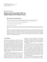
Since the y component of the first signal includes two
frequency components, phase synchrony between x and u

should be observed at the IMFs with the mean frequencies,
f
1
= 0.65 and f
2
= 0.25 Hz. 100 simulations of the model is
generated with additive white Gaussian noise at a SNR value
of 10 dB. The largest two synchrony values with mean and
standard de viations, 0.5109
± 0.0427 and 0.9482 ± 0.0361,
are obtained at the 5th and 6th IMFs which oscillate at the
mean frequencies 0.65 and 0.25 Hz, respectively. This result
is consistent with the model where the synchrony provided
by the 6th IMF is greater than the one provided by the 5th
IMF, since C
2
is greater than C
1
. A sample decomposition
of x, y, u and v into their IMFs using MEMD is given in
Figure 1.
4.2. Rossler Oscillator Model. In the remainder of the paper,
in order to evaluate the performance of the proposed
multivariate measures, a well-known model of nonlinear
oscillators, called Rossler oscillators, is used. These chaotic
oscillators, investigated by [2, 35], form a system that is
known to have characteristic phase synchronization prop-
erties and to exhibit clusters of phase synchronization
depending on the coupling strengths within the system.
The model consists of a network of multivariate time series

coupled in a way to form synchronization clusters of different
size as well as desynchronized oscillators. The networks
considered in this paper consist of N
= 6 Rossler oscil lators
which are coupled diffusively via their z-components:
˙
x
j
= 10

y
j
− x
j

,
˙
y
j
= 28x
j
− y
j
− x
j
z
j
,
˙
z

j
=−
8
3z
j
+ x
j
y
j
+
N

i=1

ij

z
i
− z
j

.
(9)
The coupling coefficients,

ij
, are chosen from the inter-
val [0, 1] to construc t different networks. The differential
equations are numerically integrated using the Runge-Kutta
method with a time step of Δt

= 1/25 sec corresponding to a
sampling frequency of 25 Hz, where the initial conditions are
randomly chosen from the interval, [0, 100]. The first 2500
samples are discarded to eliminate the initial transients.
4.3. Comparison of Direct Application of Hilbert Transform
with Multivariate EMD. Inordertoillustratetheadvantage
of using multivariate EMD as a preprocessing tool over the
direct application of the Hilbert transfor m in estimating the
time-varying phase synchrony, the Rossler network in (9)
is simulated using 1300 samples ( see Figure 4(a)), where
the coupling strengths,

1,2
= 
2,1
= 
1,3
= 
3,1
=

2,3
= 
3,2
= 1, 
4,5
= 
5,4
= 
4,6

= 
6,4
= 
5,6
=

6,5
= 1 and all other coupling strengths are set to zero,
such that the network consists of two strongly synchronized
clusters with no between-cluster coupling. The first cluster
is shown in green and the second cluster is shown in yellow
in Figure 4(a). In this example, three S values representing
the phase synchrony within the clusters (green, yellow,
and the whole network) and the R
v
value representing the
synchrony between the clusters are computed. In the absence
of noise, when the phase synchrony analysis is performed
for the z-components of the Rossler oscillators using the
Hilbert transform, S and R
v
values are computed as S
g
= 1
EURASIP Journal on Advances in Signal Processing 7
−2
0
2
−2
0

2
−2
0
2
−2
0
2
−2
0
2
−2
0
2
−2
0
2
IMF
1
IMF
2
IMF
3
IMF
4
IMF
5
IMF
6
IMF
7

IMF
8
xy
uv
−1
0
1
−1
0
1
−1
0
1
−1
0
1
−1
0
1
−1
0
1
−1
0
1
−0.5
0
0.5
−0.5
0

0.5
−0.5
0
0.5
−0.5
0
0.5
−0.5
0
0.5
−0.5
0
0.5
−5
0
5
−5
0
5
−5
0
5
−5
0
5
−5
0
5
−5
0

5
−5
0
5
−0.1
0
0.1
0 500
0 500
0 500
0
500
0 500
0 500
0 500
0 500
0500
0500
0500
0
500
0500
0500
0500
0500
0500
0500
0500
0
500

0500
0500
0500
0500
0500
0500
0500
0
500
0500
0500
0500
0500
−0.2
0
0.2
−0.2
0
0.2
−0.2
0
0.2
0
0.2
0.4
t (s) t (s) t (s) t (s)
Figure 1: Decomposition of x, y, u,andv in (8) into the IMFs by MEMD: 5th and 6th IMFs which oscillate at mean frequencies 0.65 and
0.25 Hz, respectively, provide the largest synchrony values between x and u.
8 EURASIP Journal on Advances in Signal Processing
1

2
3
4
5
6
ρ
1
ρ
2
Figure 2: Rossler network for evaluating the dependency of the
multivariate synchrony measures on the coupling strengths. The
coupling strengths ρ
1
and ρ
2
are increased from 0 to 1 in steps of 0.2.
(S value computed for the first cluster), S
y
= 1(second
cluster), S
T
= 0.6175 (network consisting of all 6 oscillators),
and R
v
= 0.007. These values agree with our intuition, since
the S-estimator is proportional to the amount of within-
cluster synchronization and R
v
-estimator is proportional to
the amount of between-cluster synchronization. However,

Hilbert transform is actually a filter with unit gain at ever y
frequency [2], so that the whole range of frequencies is taken
into account to define the instantaneous phase. Therefore,
if the signal is broadband it is necessary to prefilter it in
the frequency band of interest before applying the Hilbert
transform, in order to get an accurate estimate of the phase
(e.g., [8, 9]). Therefore, instead of bandpass filtering the
oscillators, multivariate EMD will be employed, and for the
Rossler networks, the IMFs with the highest energies will be
used for the synchrony analysis, since these networks consist
of monocomponent oscillators.
To show the advantage of using multivariate EMD, 50
simulations of the Rossler network are performed with
additive white Gaussian noise at a SNR value of 0 dB. When
the Hilbert transform is used directly, the mean values and
the standard deviations of the S and R
v
estimators are
computed as S
g
= 0.1651 ± 0.0162, S
y
= 0.1617 ± 0.0172,
S
T
= 0.1069±0.0095, and R
v
= 0.1413±0.0243. These results
are not close to the ideal values of S and R
v

estimators given
above. This is caused by the broadband nature of the noise
and the fact that the Hilbert transform is actually a filter with
unit gain at every frequency. However, when multivariate
EMD is used and the IMFs with the highest energies are
extracted from each oscillator, the mean values and the
standard deviations (mean
± std) of the S and R
v
estimators
are computed as S
g
= 0.7888 ± 0.0377, S
y
= 0.7771 ± 0.0349,
S
T
= 0.5144±0.0362, and R
v
= 0.1214±0.0653. These results
are much closer to the ideal values of S and R
v
, which shows
the advantage of using multivariate EMD as a preprocessing
tool for phase synchrony analysis.
4.4. Performance of Multivariate Synchrony Measures for
Multivariate EMD. In this example, the dependency of the
multivariate synchrony measures on the coupling strengths
in a Rossler network is evaluated using 500 samples. The
network in Figure 2 is formed, and the coupling strengths

ρ
1
= 
1,4
= 
4,1
and ρ
2
= 
2,6
= 
6,2
are increased from 0 to 1
in steps of 0.2, with

1,2
= 
2,1
= 
1,3
= 
3,1
= 
2,3
= 
3,2
= 1,

4,5
= 

5,4
= 
4,6
= 
6,4
= 
5,6
= 
6,5
= 1, and all other
coupling strengths set to zero.
Figure 3 shows the dependency of the S
g
, S
y
, S
T
,and
R
v
on the coupling strengths ρ
1
and ρ
2
, in the absence
of noise. When both ρ
1
and ρ
2
are equal to zero, S

g
and
S
y
have the highest values, which is equivalent to the
network in Figure 4(a). In this case, there are two completely
separate clusters, and each cluster has the maximum phase
synchrony, with no between-cluster synchrony. This result
is expected, since the S values represent the within-cluster
phase synchrony and increasing the coupling coefficients ρ
1
and ρ
2
synchronizes the two of the oscillators from each
cluster to the other two oscillators in the other cluster,
which destroys the within-cluster phase synchrony. Thus,
maximum within-cluster synchrony is achieved when ρ
1
= 0
and ρ
2
= 0 and increasing either or both ρ
1
and ρ
2
results in
the reduced within-cluster phase synchrony values, shown by
Figures 3(a) and 3(b).
S
T

, which shows the within-cluster synchrony for the
whole network, has the maximum value when ρ
1
and ρ
2
are
both equal to 1. This is also an expected result since these two
coupling strengths try to synchronize the two clusters with
each other. Reduction in either or both of ρ
1
and ρ
2
results in
a reduced S
T
value, which is shown in Figure 3(c).
Figure 3(d) shows that R
v
, which represents the between-
cluster synchrony, is directly proportional to ρ
1
and ρ
2
.
An increase in only one of the coupling strengths is
not enough to increase R
v
. However, when both of these
coupling strengths increase, R
v

also increases and reaches its
maximum value when ρ
1
= 1andρ
2
= 1. This is an expected
result since both ρ
1
and ρ
2
are responsible for the increased
between-cluster synchrony. Moreover, by looking at Figures
3(c) and 3(d), one can say that there is a strong positive
correlation between S
T
and R
v
. The reason for this is that R
v
represents the between-cluster synchrony and S
T
represents
the synchrony, of the whole network, both of which increase
with the increasing coupling strengths, ρ
1
and ρ
2
.
In order to evaluate the performance of the S-andR
v

-
estimators in estimating the within-cluster and between-
cluster synchrony in detail, 12 different Rossler networks,
shown in Figure 4, consisting of 6 oscillators are gener-
ated. Each connection represents two symmetric coupling
strengths, equal to 1, between two oscillators. The z-
components of the oscill ators are preprocessed by the
multivariate EMD, and the IMFs with the highest energies
are extracted from each oscillator. The IMFs with the
highest energies correspond to the same mode for all 6
oscillators. For each network, 50 simulations are performed
with additive white Gaussian noise at a SNR value of 0 dB.
Table 1 shows the mean and standard deviation values
for all 12 networks. Networks 1 and 5 have the largest
S
g
and S
y
values, which indicates that the within-cluster
EURASIP Journal on Advances in Signal Processing 9
ρ
1
ρ
2
Dependency of the S
g
on the coupling strengths
0
0.2
0.4

0.6
0.8
1
0 0.2
0.4
0.6 0.8 1
0.7
0.75
0.8
0.85
0.9
0.95
(a) S
g
ρ
1
ρ
2
Dependency of the S
y
on the coupling strengths
0
0.2
0.4
0.6
0.8
1
0 0.2 0.4 0.6 0.8 1
0.7
0.75

0.8
0.85
0.9
0.95
(b) S
y
ρ
1
ρ
2
Dependency of the S
T
on the coupling strengths
0
0.2
0.4
0.6
0.8
1
0 0.2 0.4 0.6 0.8 1
0.45
0.5
0.55
0.6
0.65
(c) S
T
ρ
1
ρ

2
Dependency of the R
v
on the coupling strengths
0
0.2
0.4
0.6
0.8
1
0 0.2 0.4
0.6
0.8
1
0.1
0.2
0.3
0.4
0.5
0.6
(d) R
Figure 3: Dependency of the multivariate synchrony measures, S
g
, S
y
, S
T
,andR
v
, on the coupling strengths ρ

1
and ρ
2
.
Table 1: Means and standard deviations of R
v
, S
g
, S
y
,andS
T
for the networks in Figure 4.
R
v
S
g
S
y
S
T
Network 1 0.2131 ± 0.1786 0.7670 ± 0.0631 0.7827 ± 0.0665 0.5390 ± 0.0668
Network 2 0.1306
± 0.0961 0.3605 ± 0.2239 0.4490 ± 0.2556 0.2881 ± 0.1183
Network 3 0.1476
± 0.1364 0.5826 ± 0.1342 0.5641 ± 0.1230 0.4038 ± 0.0763
Network 4 0.6160
± 0.2165 0.6398 ± 0.1445 0.6644 ± 0.1375 0.5947 ± 0.1487
Network 5 0.9380
± 0.0266 0.7687 ± 0.0527 0.7631 ± 0.0594 0.7956 ± 0.0491

Network 6 0.7539
± 0.3110 0.4130 ± 0.2489 0.4153 ± 0.2409 0.5047 ± 0.2446
Network 7 0.6913
± 0.2354 0.4735 ± 0.1945 0.4876 ± 0.2016 0.5175 ± 0.1884
Network 8 0.2350
± 0.1687 0.3046 ± 0.2004 0.2944 ± 0.1997 0.2624 ± 0.1537
Network 9 0.4376
± 0.1319 0.4070 ± 0.0881 0.4192 ± 0.0959 0.4164 ± 0.0671
Network 10 0.7774
± 0.0695 0.4056 ± 0.0946 0.3941 ± 0.0976 0.5305 ± 0.0761
Network 11 0.3479
± 0.1374 0.4043 ± 0.0879 0.4046 ± 0.0818 0.3996 ± 0.0566
Network 12 0.4196
± 0.1361 0.4092 ± 0.0836 0.1777 ± 0.0912 0.3455 ± 0.0629
10 EURASIP Journal on Advances in Signal Processing
1
2
3
4
5
6
(a) Network 1
1
2
3
4
5
6
(b) Network 2
1

2
3
4
5
6
(c) Network 3
1
2
3
4
5
6
(d) Network 4
1
2
3
4
5
6
(e) Network 5
1
2
3
4
5
6
(f) Network 6
1
2
3

4
5
6
(g) Network 7
1
2
3
4
5
6
(h) Network 8
1
2
3
4
5
6
(i) Network 9
1
2
3
4
5
6
(j) Network 10
1
2
3
4
5

6
(k) Network 11
1
2
3
4
5
6
(l) Network 12
Figure 4: 12 different Rossler networks for evaluating the performance of the S-andR
v
-estimators in estimating the within-cluster and
between-cluster synchrony. Each node represents an oscillator, and each connection represents the two symmetric coupling strengths, which
are equal to 1, between two oscillators.
phase synchrony is very strong for these networks. Strong
within-cluster synchrony, or high S value, is usually obtained
when all possible within-cluster connections exist and
the between-cluster connections are either very strong or
nonexistent. Networks 1 and 5 satisfy these conditions
with network 1 having no between-cluster connections and
network 5 having strong connections between the two
clusters. On the other hand, networks 3 and 4 have all
possible within-cluster connections, but they have smaller
S
g
and S
y
values compared to network 5, since the small
number of between-cluster connections are not adequate to
synchronize the two clusters and are also disruptive to the

within-cluster synchrony.
The largest R
v
value, or between-cluster synchrony, is
observed for network 5 which results from the three connec-
tions between the two clusters, forcing the two clusters to be
highly synchronized with each other. Networks 6 and 10 also
have a large number of connections between the two clusters
but they lack some of the within-cluster connections, which
results in reduced R
v
values for these networks. Network
6 has a larger R
v
value compared to network 7 but has
smaller S values, since there are 3 connections between
the clusters. Networks 8, 9, 11, and 12 all have smal l R
v
and S values, since the within-cluster and between-cluster
synchronies are both weak due to the lack of connectivity in
these networks.
S
T
, on the other hand, measures the within-cluster
synchronization when all six oscillators are assumed to form
a big cluster. Network 5 has the largest S
T
value, because
there is one big cluster which is formed by multiple smaller
clusters with strong within-cluster connectivity. Since the

connectivity in the whole network is strong, the eigenvalues
of the synchrony matrix tend to be better concentrated,
which results in a low entropy value and a high S
T
value. On
the other hand, networks 2 and 8 have small S
T
values, since
the within-network connectivity is not st rong.
EURASIP Journal on Advances in Signal Processing 11
4.5. Significance Testing for the Multivariate Synchrony
Measures. Determining the statistical significance involves
hypothesis testing and requires the formation of a null
hypothesis. In some cases, it may be possible to derive ana-
lytically the distribution of the given measure under a given
null hypothesis. However, in the case of the multivariate
synchronization measures, this proves to be a very difficult
problem, therefore this distribution is estimated by direct
Monte Carlo simulations. For this purpose, an ensemble of
surrogate data sets are generated [36]. The surrogate data
set is generated by first computing the Fourier transform of
the data and then randomizing the phase. Finally, the inverse
Fourier transform is taken to obtain the surrogate data which
has the same power spectrum and autocorrelation function
as the original data. This operation preserves the amplitude
relationships while randomizing the phase dependencies. For
each surrogate data set, the MEMD is applied, the IMFs are
extracted, and the corresponding multivariate measures are
computed. From this ensemble of statistics, the distribution
is approximated. A robust way to define significance would

be directly in terms of the P-values with rank statistics. For
example, if the observed time series has a R
v
or S value, that
is in the lower one percentile of all the surrogate statistics,
then a P-value of P
= .01 could be quoted. For the networks
in Figure 3, 100 surrogate data sets are formed, and all
multivariate synchrony measures, R
v
, S
g
, S
y
,andS
T
,are
found to be significant at P
= .05. The surrogate testing
demonstrates that our simulation results are not likely to
occur by chance.
4.6. Application to EEG Data. The proposed multivariate
phase synchronization measures in conjunction with multi-
variate EMD were applied to a set of EEG data containing
the error-related negativity (ERN). The ERN is a brain
potential response that occurs following performance errors
in a speeded reaction time task [37]. Previous work [38]
indicates that there is increased phase synchrony associated
with ERN for the theta frequency band (4–7 Hz) and
ERN time window (25–75 ms) between frontal and central

electrodes versus central and parietal. EEG data from 63-
channels was collected in accordance with the 10/20 system
on a Neuroscan Synamps2 system (Neuroscan, Inc.) (The
authors would like to acknowledge Dr. Edward Bernat from
Florida State University for sharing his EEG data with us). A
speeded-response flanker task was employed, and response-
locked averages were computed for each subject.
Inthispaper,weanalyzeddatafrom11subjects
corresponding to the error responses from five electrodes
corresponding to the areas of interest, that is, two frontal
electrodes (F3 and F4), one central electrode (FCz), and
two parietal electrodes (CP3 and CP4). All five electrodes
were first transformed using multivariate EMD, and the
IMF closest to the theta frequency band was selected.
The five IMFs were used to estimate phase and compute
the pairwise phase synchrony. After the 5
× 5bivariate
synchronization matrix was formed, we computed S and R
v
values considering two groups of electrodes, F3, F4, and FCz
and CP3, CP4, and FCz.
For all 11 subjects, S value of the electrode group, F3-
F4-FCz, is larger than the S value of the group, CP3-CP4-
FCz. A Wilcoxon rank sum test is used at %5 significance
level to test the null hypothesis that the S values of the
group F3-F4-FCz and the S values of the group CP3-CP4-
FCz are independent samples from identical distributions
with equal medians, against the alternative that they do
not have equal medians. T he P-value provided by the test
is .0215, which is less than .05. Thus, the null hypothesis

is rejected at 5% significance level, which shows that the
S values of the group F3-F4-FCz are significantly larger
than the S values of the group CP3-CP4-FCz. This result
indicates that the frontal (F3 and F4) electrodes are more
strongly coupled to the central electrode (FCz), compared
to the coupling between the parietal (CP3 and CP4) and
central electrodes, which is show n by the significantly larger
within-cluster synchrony values. Moreover, R
v
value between
the central-frontal and R
v
value between the central-parietal
electrode groups are computed. R
v
value between the central-
frontal electrodes is larger for 10 subjects out of 11. Using the
Wilcoxon rank sum test, the null hypothesis is rejected with
P-value
= .0181, which demonstrates that the synchrony
between the frontal (F3 and F4) electrodes and central
electrode (FCz) is larger compared to the synchrony between
the parietal (CP3 and CP4) and central electrodes, which is
shown by the significantly larger between-cluster synchrony.
These results are consistent with the previous work in
[38].
5. Conclusions
In this paper, a new approach for quantifying multivariate
phase synchronization within a group of oscillators as well
as between groups has been introduced. The proposed

approach is based on the application of multivariate empiri-
cal mode decomposition for extracting time- and frequency-
dependent phase information, and adapting measures of
correlation from statistics to multivariate analysis. The pro-
posed approach offers improvements over existing methods
in two ways. First, the MEMD is data driven in the sense
that it extracts modes or frequencies that are common
to all of the signals under consideration, thus eliminating
the need for arbitrarily chosen bandpass filters as in the
case of the Hilbert and the wavelet transforms. The time-
varying phase information extracted through MEMD reflects
the underlying nature of the signals and is more efficient
compared to standard t ransform based approaches where
each frequency is considered regardless of its impor tance.
Second, the proposed approach extends the current state of
the art-phase synchrony analysis from quantifying bivariate
relationships to multivariate ones. This shift from pairwise
bivariate synchrony analysis to multivariate analysis within
andacrossgroupsoffers advantages especially for complex
system analysis such as the brain, where the bivariate
relationships do not always reflect the underlying network
structure. The multivariate synchrony measures, such as the
ones introduced in this paper, are a step in the right direction
for understanding the network dynamics.
12 EURASIP Journal on Advances in Signal Processing
Future work will focus on the extension of the proposed
measures using different multivariate analysis techniques
such as cluster analysis and canonical correlation to obtain
a more detailed understanding of the synchronization net-
works as well as the application of these measures to a

large number of signals, as is the case with EEG. In the
current application to EEG data, we focused on a group of
electrodes with known synchronization patterns. It would be
valuable to apply the proposed approach to the whole set
of electrodes and discover the underly ing synchronization
clusters through a combination of eigenvalue decomposition
and measures of association and complexity, for example, R
v
and S.
Acknowledgment
This paper was in part supported by grants from the National
Science Foundation under CCF-0728984 and CAREER CCF-
0746971.
References
[1] E. Pereda, R. Q. Quiroga, and J. Bhattacharya, “Nonlinear
multivariate analysis of neurophysiological signals,” Progress in
Neurobiology, vol. 77, no. 1-2, pp. 1–37, 2005.
[2]M.G.Rosenblum,A.S.Pikovsky,andJ.Kurths,“Phase
synchronization of chaotic oscillators,” Physical Review Letters,
vol. 76, no. 11, pp. 1804–1807, 1996.
[3] P. Tass, M. G. Rosenblum, J. Weule et al., “Detection of n:m
phase locking from noisy data: application to magnetoen-
cephalography,” Physical Review Letters, vol. 81, no. 15, pp.
3291–3294, 1998.
[4] J. P. Lachaux, A. Lutz, D. Rudrauf et al., “Estimating the
time-course of coherence between single-trial brain signals: an
introduction to wavelet coherence,” Neurophysiologie Clinique,
vol. 32, no. 3, pp. 157–174, 2002.
[5] S. Mallat, A Wavelet Tour of Signal Processing, Academic Press,
New York, NY, USA, 1999.

[6] M. Le Van Quyen, J. Foucher, J. P. Lachaux et al., “Comparison
of Hilbert transform and wavelet methods for the analysis
of neuronal synchrony,” Journal of Neuroscience Methods, vol.
111, no. 2, pp. 83–98, 2001.
[7] L. Angelini, M. De Tommaso, M. Guido et al., “Steady-
state visual evoked potentials and phase synchronization in
migraine patients,” Physical Review Letters, vol. 93, no. 3,
Article ID 038103, 2004.
[8] J. Bhattacharya, “Reduced degree of long-range phase syn-
chrony in pathological human brain,” Acta Neurobiologiae
Experimentalis, vol. 61, no. 4, pp. 309–318, 2001.
[9] M. Koskinen, T. Sepp
¨
anen, J. Tuukkanen, A. Yli-Hankala, and
V. J
¨
antti, “Propofol anesthesia induces phase synchronization
changes in EEG,” Clinical Neurophysiology, vol. 112, no. 2, pp.
386–392, 2001.
[10] T. M. Rutkowski, D. P. Mandic, A. Cichocki, and A. W.
Przybyszewski, “EMD approach to multichannel EEG data—
the amplitude and phase components clustering analysis,”
Journal of Circuits, Systems and Computers,vol.19,no.1,pp.
215–229, 2010.
[11]C.M.Sweeney-ReedandS.J.Nasuto,“Anovelapproachto
the detection of synchronisation in EEG based on empirical
mode decomposition,” Journal of Computational Neuroscience,
vol. 23, no. 1, pp. 79–111, 2007.
[12] D. Looney, C. Park, P. Kidmose, M. Ungstrup, and D. P.
Mandic, “Measuring phase synchrony using complex exten-

sions of EMD,” in Proceedings of the IEEE/SP 15th Workshop on
Statistical Signal Processing (SSP ’09), pp. 49–52, August 2009.
[13] T. Tanaka and D. P. Mandic, “Complex empirical mode
decomposition,” IEEE Signal Processing Letters, vol. 14, no. 2,
pp. 101–104, 2007.
[14] M. Bin Altaf, T. Gautama, T. Tanaka, and D. P. Mandic, “Rota-
tion invariant complex empirical mode decomposition,” in
Proceedings of the IEEE International Conference on Acoustics,
Speech and Signal Processing (ICASSP ’07), vol. 3, pp. 1009–
1012, April 2007.
[15] G. Rilling, P. Flandrin, P. Goncalves, and J. M. Lilly, “Bivariate
empirical mode decomposition,” IEEE Signal Processing Let-
ters, vol. 14, no. 12, pp. 936–939, 2007.
[16] D. Looney and D. P. Mandic, “Multiscale image fusion using
complex extensions of EMD,” IEEE Transactions on Signal
Processing, vol. 57, no. 4, pp. 1626–1630, 2009.
[17] N. Rehman and D. Mandic, “Empirical mode decomposition
for trivariate signals,” IEEE Transactions on Signal Processing,
vol. 58, no. 3, pp. 1059–1068, 2010.
[18] N. Rehman and D. P. Mandic, “Multivariate empirical mode
decomposition,” Proceedings of the Royal Society A: Mathemat-
ical, Physical and Engineering Sc iences, vol. 466, no. 2117, pp.
1291–1302, 2010.
[19] B. Schelter, M. Winterhalder, R. Dahlhaus, J. Kurths, and
J. Timmer, “Partial phase synchronization for multivariate
synchronizing systems,” Physical Review Letters, vol. 96, no. 20,
Article ID 208103, 2006.
[20] M. E. J. Newman, “Finding community structure in networks
using the eigenvectors of matrices,” Physical Review E -
Statistical, Nonlinear, and Soft Matter Physics, vol. 74, no. 3,

Article ID 036104, 2006.
[21] M. E. J. Newman, “Modularity and community structure in
networks,” Proceedings of the National Academy of Sciences of
the United States of America, vol. 103, no. 23, pp. 8577–8582,
2006.
[22] C. Allefeld and J. Kurths, “An approach to multivariate phase
synchronization analysis and its application to event-related
potentials,” International Journal of Bifurcation and Chaos, vol.
14, no. 2, pp. 417–426, 2004.
[23] C. Allefeld, M. M
¨
uller, and J. Kurths, “Eigenvalue decom-
position as a generalized synchronization cluster analysis,”
International Journal of Bifurcation and Chaos, vol. 17, no. 10,
pp. 3493–3497, 2007.
[24] C. Allefeld, S. Frisch, and M. Schlesewsky, “Detection of early
cognitive processing by event-related phase synchronization
analysis,” NeuroReport, vol. 16, no. 1, pp. 13–16, 2005.
[25] C. Allefeld and J. Kurths, “Multivariate phase synchronization
analysis of EEG data,” IEICE Transactions on Fundamentals of
Electronics, Communications and Computer Sciences, vol. 86,
no. 9, pp. 2218–2221, 2003.
[26] C. Allefeld and S. Bialonski, “Detecting synchronization
clusters in multivariate time series via coarse-graining of
Markov chains,” Physical Review E, vol. 76, no. 6, Article ID
066207, pp. 66207–66215, 2007.
[27] C. W. J. Granger, “Investigating causal relations by economet-
ric models and cross-spectral methods,” Econometrica, vol. 37,
no. 3, pp. 424–438, 1969.
[28] L. A. Baccal

´
a and K. Sameshima, “Partial directed coherence:
a new concept in neural structure determination,” Biological
Cybernetics, vol. 84, no. 6, pp. 463–474, 2001.
EURASIP Journal on Advances in Signal Processing 13
[29] P. Robert and Y. Escoufier, “A unifying tool for linear
multivariate statistical methods: the RV-coefficient,” Applied
Statistics, vol. 25, no. 3, pp. 257–265, 1976.
[30] K. Oshima, C. Carmeli, and M. Hasler, “State change detection
using multivariate synchronization measure from physiologi-
cal signals,” Journal of Signal Processing, vol. 10, no. 4, pp. 223–
226, 2006.
[31] N. E. Huang, Z. Shen, S. R. Long et al., “The empirical mode
decomposition and the Hubert spectrum for nonlinear and
non-stationar y time series analysis,” Proceedings of the Royal
Society A: Mathematical, Physical and Engineering Sciences, vol.
454, no. 1971, pp. 903–995, 1998.
[32] D. Mandic and V. Goh, Complex Valued Nonlinear Adaptive
Filters: Noncircularity, Widely Linear and Neural Models,Wiley
Publishing, 2009.
[33] R. Horn and C. Johnson, Matrix Analysis, Cambridge Univer-
sity Press, Cambridge, UK, 1990.
[34] M. Chavez, C. Adam, V. Navarro, S. Boccaletti, and J.
Martinerie, “On the intrinsic time scales involved in synchro-
nization: a data-driven approach,” Chaos,vol.15,no.2,Article
ID 023904, pp. 1–11, 2005.
[35] G. V. Osipov, A. S. Pikovsky, M. G. Rosenblum, and J. Kurths,
“Phase synchronization effects in a lattice of nonidentical
R
¨

ossler oscillators,” Physical Review E, vol. 55, no. 3, pp. 2353–
2361, 1997.
[36] D. Prichard and J. Theiler, “Generating surrogate data for
time series with several simultaneously measured variables,”
Physical Review Letters, vol. 73, no. 7, pp. 951–954, 1994.
[37] J. R. Hall, E. M. Bernat, and C. J. Patrick, “Externalizing psy-
chopathology and the error-related negativity,” Psychological
Science, vol. 18, no. 4, pp. 326–333, 2007.
[38] J. F. Cavanagh, M. X. Cohen, and J. J. B. Allen, “Prelude to and
resolution of an error: EEG phase synchrony reveals cognitive
control dynamics during action monitoring,” Journal of
Neuroscience, vol. 29, no. 1, pp. 98–105, 2009.