Advances in Solid-State Lasers: Development and Applicationsduration and in the end limits Part 5 docx
Bạn đang xem bản rút gọn của tài liệu. Xem và tải ngay bản đầy đủ của tài liệu tại đây (3.81 MB, 40 trang )
Advances in Solid-State Lasers: Development and Applications
152
Fig. 4-3. long term ice-cloud measurement. January 24, 2009. Temp. 3.7deg Hum. 70% Cloudy
In-line Typed High-Precision Polarization Lidar for Disaster Prevention
153
1000
0
Altitude [m]
0
1
Fig. 4-4. lidar echoes (p-components) in bad weather condition. (a) July 4, 2006. Temp. 28deg.
Hum. 52%. Before heavy rain (b) July 14, 2006, Temp. 32deg. Hum. 50% Thunder cloud
proportional to the product of the ionization electron density n
e
and the magnetic flux density
B along the beam propagation path. The linearly polarized beam can be regarded as a
combination of the clockwise and the counterclockwise circularly polarized beams. The
refractive indices of the ionized atmosphere for each circularly polarized beam are as follows.
1/2
2
2
2
0
1
pe
ce
e
pe ce
ee
n
en eB
mm
ω
ω
ωωω
ωω
ε
±
⎛⎞
=−
⎜⎟
⎜⎟
±
⎝⎠
==
(5-1)
where
p
e
ω
,
ce
ω
are the plasma and electron cyclotron frequencies, respectively, e is the
fundamental charge, m
e
is the electron mass, and
0
ε
is the permittivity of free space.
Therefore, the rotation angle of polarization of the beam propagated at distance L (=L
1
~L
2
) is
obtained as follows.
2
1
2
1
13 2
()
2.62 10
L
L
L
e
L
nndl
nBdl
π
δ
λ
λ
+−
−
=−
=×
∫
∫
(5-2)
Advances in Solid-State Lasers: Development and Applications
154
where
λ
is wavelength of the propagating beam. Since
δ
is proportional to
λ
2
, the rotation
angle for visible light is small. Therefore, the polarization angle rotation must be measured
with high accuracy in order to detect lightning discharge.
When the Faraday effect is applied to lightning measurement, the atmosphere needs to be
partially ionized, and the magnetic flux due to the lightning discharge must exist. Cloud-to-
cloud discharge, which causes 20-30 times continuous discharge, satisfies those conditions.
(Franzblau & Popp, 1989; Franzblau, 1991; Stith et al, 1999; Society of Atmospheric
Electricity of Japan, 2003)
Magnetic Flux
Density B
Partially Ionized
A
tmosphere/Cloud
Linearly
Polarized Beam
Rotation Angle
δ
Fig. 5-1. Faraday effect.
5.2 New concept lidar
The analysis and experimental results have shown that the rotation angle of polarization
plane of the propagating beam is less than 1 degree, so that the mutually perpendicular
polarization components must be measured with a sensitivity and accuracy of >30 dB in
order to detect lightning discharges. The rotation of the polarization plane only occurs in a
nearly perfectly ionized atmosphere, so the signal cannot be detected unless the transmitted
beam intersects the discharge path. On the other hand, the shock wave (variation in the
neutral gas density) generated by the discharge can be detected over a broader range, while
it causes no rotation of the polarization plane. (Fukuchi, 2005)
This was confirmed by high
voltage discharge experiment in the next section.
Therefore, the scenario of the lightning detection using the lidar system is designed as
follows. At first the system roughly scans the sky in the direction in which the occurrence of
a cloud-to-cloud lightning discharge is likely. If a shock wave is detected, the 3-demensional
lightning position is estimated. Next, by scanning the neighborhood of the lightning
position with higher precision to intersect the propagating beam and the lightning discharge
path, the rotation angle of the polarization plane is measured. In general, lower area
(bottom) of clouds will be scanned, as the beam penetrates only a few hundred meters in
clouds. The distribution of the discharge location and its change will lead to the prediction
of lightning strike.
In-line Typed High-Precision Polarization Lidar for Disaster Prevention
155
The lidar system must be capable of measurement at near range with a narrow field of view
in order to eliminate the effects of multiple scattering. The use of in-line optics is effective in
meeting this requirement. The system must also have scanning capability to search the
cloud-to-cloud lightning discharge. The concept of the lidar system for lightning detection is
shown in Fig.5-2. For the detection of the small rotation angle, differential detection should
be used.
PMT
PMT
A
mp.
A
mp.
Differential
A
mp.
Oscilloscope
Transmitting / Receiving
Telescope
Laser
Trigger
Thunder Cloud
Partially Ionized
A
tmosphere
Optical
Circulator
Fig. 5-2. Concept of lidar lightning detection.
6. Demonstration –Ground based experiment-
6.1 Apparatus
Figure 6-1 shows the experimental setup of the high-voltage discharge experiment. (Shiina,
2008b; Fukuchi, in press) The experiment was conducted in a high voltage experiment hall
using an impulse voltage generator (HAEFELY SGΔΑ1600-80). The discharge gap between
the needle electrodes was 0-2 m and the charging voltage was >1000 kV. A voltage divider
and Rogowski coil were used to measure the charge voltage and the discharge current. The
laser beam was transmitted near the discharge path. The polarization plane of the linearly
polarized laser beam was so adjusted by a half wave plate (HWP) that its photon flux was
equally divided into the two mutually orthogonal polarization components. The intensities
of the orthogonal polarization components were detected by photodiodes (PDs) with
amplifiers. A differential amplifier was also installed in the receiver circuit to detect the
small rotation angle of the polarization plane. To eliminate electromagnetic noise caused by
the discharge, the laser power supply and the receiver circuit were placed inside copper
boxes. Signal cables were also shielded by wire mesh. The specifications of the discharge
equipment and the optical detection system are summarized in Table 6-1. The differential
output was detected only when the polarization plane was rotated by the Faraday effect.
Advances in Solid-State Lasers: Development and Applications
156
The position of the propagating beam could be adjusted with respect to the discharge path
and the discharge terminals.
The rotation angle of the polarization plane was estimated from the intensities of the
orthogonal polarization components or the differential output by eq.(6-1). I
p
and I
s
are the
intensities of the orthogonal polarization components.
1
1
tan ( / )
4
tan ( )
s
p
pS
PS
II
II
II
π
δ
−
−
=−
−
=
+
(6-1)
PD
PD
Pre-Amp.
Diff Amp.
Oscilloscope
High-Voltage
Power Supply
high voltage
needle electrode
Laser
150mW@532nm
HWP
Polarizer
Discharge
Path
Beam propagation
len
g
th >30 m
Charge voltage +/-600kV - +/-1200kV
Dischar
g
e current - 3kA
ground
needle electrode
Fig. 6-1. Experimental setup of the high voltage discharge experiment.
When |Ip-Is|<<Ip, Is, the rotation angle is approximated by the following equation.
sp
sp
II
II
+
−
=
δ
(6-2)
The estimation of the rotation angle is illustrated in Fig. 6-2. The polarity of the rotation
angle indicates the spatial relation between the beam and the discharge path.
Is
Ip
P
S
δ
: Rotation Angle
Polarization of beam
rotated by discharge
Polarization of transmitted
laser beam
Fig. 6-2. Differential detection.
In-line Typed High-Precision Polarization Lidar for Disaster Prevention
157
Discharge equipment
Manufacturer, model
HAEFELY SG ΔΑ1600-80
Maximum charging voltage +/-1600 kV
Discharge waveform Lightning Impulse
Electrodes needles
Discharge gap length 0-2 m
Beam/Receiver
Light source Nd:YAG green laser
λ=532 nm, CW
Power 150 mW
Detector Photodiode + Amplifier
detection Differential detection
Table 6-1. Specifications of the discharge equipment and the optical detection system
6.2 Rotation angle detection
6.2.1 Detection of shock waves
Lightning discharge generates shock waves, which accompany variations in the air density
and cause fluctuations of the propagating beam.(Fukuchi, 2005) Signals due to the shock
waves are shown in Fig. 6-3. The discharge gap between the needle terminals was 77 cm and
the charge voltage was –1200 kV. The propagating beam passed 4 cm below and 3 cm to the
left of the high voltage needle electrode. In this case, the rotation angle was not detected
because of the spatial separation between the discharge path and the beam. The air density
variation accompanying the shock wave does not contribute to the Faraday effect, so the
differential output is zero. In Fig. 6-3, the shock wave appeared 30 μs after the discharge
trigger, so the distance between the discharge path and the propagating beam was
calculated as 1 cm. In the experiment, we confirmed that the shock wave could be detected
at a few hundred μs after the discharge trigger. Therefore, the shock wave signal can be
used an indicator to locate the discharge location.
0 20 40 60 80
-8
-6
-4
-2
0
2
Noise
Sho ck Wa ve Si gna l
Fig. 6-3. Detection of shock wave.
Advances in Solid-State Lasers: Development and Applications
158
6.2.2 Detection of polarization rotation angle
The differential output signals corresponding to the rotation angle of the polarization plane
are shown in Fig.6-4. The typical discharge current is also shown. The discharge gap
between the needle terminals was 77 cm and the charging voltage was +/–1200 kV. The
propagating beam passed 2 cm under the high voltage needle electrode. The waveform
before 10 μs could not be evaluated because of the electromagnetic noise due to the
discharge. The differential outputs in the case of positive discharge (+1200 kV) and negative
discharge (-1200 kV) showed opposite polarity. The output signals had the same response
time as the discharge current. The rotation angle evaluated using eq. (6-1) was
δ
=0.53
degrees for positive polarity and
δ
=0.50 degrees for negative polarity. The dynamic range of
>30 dB of the differential amplifier enabled detection of the small rotation angle. The results
were in agreement with the results of numerical analysis and preliminary experiment using
short gap discharge.
0 20 40 60 80
-2
-1
0
1
2
0 20 40 60 80
0
10
20
30
0 10 20 30 40 50
-0.3
-0.2
-0.1
0
0.1
0.2
0.3
Time [μs]
1
2
3
-1 200k V
Di scha r ge C ur r ent
Noise
Fig. 6-4. Obtained waveform showing rotation angle detection for positive and negative
polarities.
To suppress the electromagnetic noise, the receiver optics and electrical circuits were put in
a shielded room. Due to spatial limitations caused by the introduction of the shield room,
the position of the propagating beam was changed to 30 cm above the ground needle
electrode from 2cm below the high voltage needle electrode. The electron density does not
change significantly in the discharge path on arc or spark discharge. The discharge gap
length was extended from 77 cm to 100 cm. This caused the shot-to-shot fluctuations of the
discharge path in the extended discharge gap. The rotation angle depends on the distance
between the discharge path and the propagating beam. Figure 6-5 shows the results of the
experiment. The discharge gap between the needle terminals was 100 cm and the charge
voltages were +1200 kV. Fig. 6-5(a) shows the differential output signals. The influence of
the electromagnetic noise on the waveform decreased in comparison with the former
experiment. Photographs of the discharge path in Fig. 6-5(b) were obtained simultaneously
with the waveforms in Fig. 6-5(a). The position of the propagating laser beam is also
indicated. The separation distance between the beam center and the discharge path was <2
In-line Typed High-Precision Polarization Lidar for Disaster Prevention
159
cm for (A) and >6 cm for (B). The rotation angle was estimated as 0.54 degrees in case (A).
The existence of the differential output is dependent on the distance between the discharge
path and the beam. The output signal thus appeared when the probing beam was located
within 2 cm apart from the discharge path, where the atmosphere was nearly perfectly
ionized (n
e
~10
25
m
-3
).
The present sensitivity of the rotation angle of the polarization plane is <1 degree. It is
sufficient to detect the rotation angle only in a perfectly ionized atmosphere (n
e
~10
25
m
-3
).
The rotation angle can be detected only if the transmitting beam crosses the neighborhood
of the discharge path. On the other hand, the shock wave does not rotate the polarization
plane, and can be detected over a broader spatial region. Therefore, the observation
algorithm for lidar application is designed as follows. At first, the lidar system roughly
scans the observation region. When a shock wave is detected, the lightning position is
estimated. Next, the neighborhood of the lightning position is scanned with higher spatial
resolution, and the rotation angle of the polarization plane is measured. The discharge
current, magnetic flux density, and ionized density of atmosphere are estimated. The
distribution of the ionized atmosphere and its change will lead to the prediction of lightning
strike.
Time [
μ
s]
Time [
μ
s]
Differential Output [V]
Differential Out
p
ut
[
V
]
(A)
(B)
(a)Differential outputs of rotation angles
Laser
Laser
(A)
(B)
(b)Snapshots of discharge path
Fig. 6-5. Discharge experiment with electromagnetic shield room.
Advances in Solid-State Lasers: Development and Applications
160
7. High precision polarization lidar
7.1 System setup
The lidar system was developed under the concept of the above lidar design. (Shiina, 2007a
& 2008c) A schematic diagram is shown in Fig. 7-1, a photograph is shown in Fig. 7-2, and
the specifications are summarized in Table 7-1. The optical circulator and a pair of Axicon
prisms were installed into the lidar optics to realize the in-line optics. All optical
components were selected to realize the high polarization extinction ratio and the high-
power light source.
The laser source is a second harmonic Nd:YAG laser of wavelength 532 nm and pulse
energy 200mJ. The polarization plane of the beam is balanced by a half wave plate (HWP) so
the intensities of the parallel (p-) and orthogonal (s-) component beams are equal. The
controlled beam passes through the specially designed polarization independent optical
circulator. The beam changes its wave shape to the annular by a pair of Axicon prisms to
expand its beam size up to the telescope diameter and to prevent the second mirror of the
telescope from blocking the beam. All of the optics including the Axicon prisms had small
tilts at the flat surface and AR coatings in every surface because the directly reflected light
goes back to the detectors. Nevertheless, gated photomultiplier tubes (PMTs) are used for
detection. The gate function stops the PMT operation until the outgoing beam exits the lidar
optics. This protects the PMTs from reflections of the high power laser pulse from optical
components in the in-line optics. The time delay between the beam firing and the start of the
gate function is 0.2 μs. In other words, the system can detect the lidar echo signals from the
near range of >30 m.
Laser Head
Optical Circulator
A
xicon Prisms
Cassegrain
Telescope
Pinhole
Scanning Mirror
Eyepiece
30 degrees
in rotation
26 degrees
in elevation
Window
PC
PMT(p) PMT(s)
Tri
gg
e
r
Oscilloscope
Fig. 7-1. Systematic diagram of high-precision polarization lidar system.
The scanning mirror was installed into the lidar system. The scanning area of the
observation was limited to 26 degrees in elevation and 30 degrees in azimuth because of the
constraint of the installation site.
In-line Typed High-Precision Polarization Lidar for Disaster Prevention
161
To detect the small rotation angle of < 1 degree, the polarization-independent optical
circulator for high power green laser was developed, as shown in Fig. 7-3. To avoid damage
from the strong incident laser pulse, half wave plates (HWP), Gran laser prisms (GLP),
Faraday rotators (FR), and mirrors (M) were chosen based on high threshold for optical
tolerance, high transmittance (high reflectance for mirrors), and high extinction ratio for the
polarization. The linearly polarized beam is divided equally at GLP1 into orthogonal
polarization beams, which go through each path and are joined together at GLP2. The
combined beam is transmitted into the Axicon prisms. When the lidar echo re-enters the
optics, the parallel (p-) polarization echo to the incident beam is detected at GLP3. The echo
Optical circulator
Axicon prisms
Laser Head
Telescope
Tube
Scanning
Mirror
Trigger
Oscilloscope
PC
Fig. 7-2. Snapshot of high precision polarization lidar system.
Laser Nd:YAG laser (Lotis TII)
Pulse Energy 200 mJ
Wavelength 532 nm
Repetition rate 10 Hz
Beam Diameter
27 cmφ
Telescope Shmidt-Cassegrain (Celestron NextarGPS)
Aperture
28 cmφ
Field of View 0.177 mrad
Detector PMT with gate function (2 ports for p- and s-polarizations)
(Hamamatsu K.K.)
Filter bandwidth 3 nm
Observation Range 0-20 km(max)
Table. 7-1. Lidar Specifications.
Advances in Solid-State Lasers: Development and Applications
162
is picked up in the direction perpendicular to the illustration. The orthogonal (s-)
polarization echo goes back into the circulator and is detected at GLP1. The isolation and the
insertion loss of the optical circulator are summarized in Table 7-2. The transmission
efficiency of the laser beam was 1.05 dB (79%) on average, which is acceptable considering
the transmittances of the optical components. It is also confirmed that the GLP had a
sufficiently high extinction ratio of >30 dB for the polarization.
p-polarization output beam
s-polarization output beam
Incident Laser (Linear polarization)
FR
HWP2
GLP2
Detector Port (s)
p-polarization echo
M
M
GLP1
GLP3
HWP1
Detector Port (p)
(perpendicular to the illustration)
s-polarization echo
M
M
Fig. 7-3. Polarization-independent optical circulator.
Isolation
Mode Pol.
Insertion
loss [dB]
p-pol. echo [dB] s-pol. echo [dB]
p
1.01
Transmitter
s
1.08
>39 >39
p
1.25 - >35.9
Receiver
s
1.65 >35.4 -
Table 7-2. Performance of polarization independent optical circulator.
7.2 Measurement
Here, echo characteristics of the high precision polarization lidar are explained in
perspective of measurement range, intensity balance between p- and s-polarization
components, and accuracy. Thanks to the in-line optics, the echo can be detected from near
range of 30-50 m. Since the near range echo is large, the receiver’s trigger is delayed by the
gate function of PMT to restrict the current, especially in the case of far range measurement.
If the PMT output current is too large, the balance between p- and s-polarizations is
disrupted. In the following figures, the delay was adjusted adequately. Echoes were
obtained from 330 m in Fig. 7-4, and from 820m in Figs. 7-5-7-7. We have confirmed that the
In-line Typed High-Precision Polarization Lidar for Disaster Prevention
163
delay of more than 3.5-4.0 μs (the lidar echo distance of 500-600 m) is acceptable to obtain
the balanced echoes.
At first, the calculated accuracy of rotation angle of the polarization plane was checked by
using a hard target. Figure 7-4 shows the p- and s-component echoes from a lightning rod
located at a distance of 480 m from the lidar. As this distance is not large enough to
eliminate the large echoes, p- and s-polarization echoes were not equal especially in near
range of <400m. The echoes were summed over 1024 shots. As the lightning rod is a
cylinder, the incident beam is depolarized if it was hit on a decline. Here we evaluated the
depolarization as the rotation angle to check the accuracy of the lidar echoes. By using the
derivation from Equation (6-1), the rotation angle was calculated as –0.497 degrees. The
negative sign indicates the clockwise rotation of polarization plane in Fig. 6-1, that is, s-
polarization component was larger than p-component. This result indicates the ability for
the detection of the small rotation angle of 1 degree.
Figure 7-5 shows the balance and the accuracy of the echo intensities in the high precision
polarization lidar by the atmospheric fluctuations. The figure shows the difference between
p- and s-component echoes summed over 4096 shots. The difference at <1 km is large, while
that at far distance becomes small, of the order of <100 μV. This difference indicates the
accuracy of rotation angle of +/-0.35. That is, the atmospheric fluctuation is restricted
enough to identify the rotation due to a lightning discharge. The accuracy, however, is
obtained under summation over a large number of shots. The lightning discharge has the
duration in the order of a 10-100 μs See Fig.6-4). Although the cloud-to-cloud discharge
continues a few dozens times, the summation should be finished within the period.
The low-altitude cloud observation is shown in Fig. 7-6. The vertical axis is the range-
corrected signal (P
L
L
2
) shown in logarithmic scale. The water cloud was detected at 2.34 km
ahead. Although p- and s-component echoes from the cloud base were equal intensity, the
difference became large at the inside of the cloud. The incident beam penetrated up to 500-
600m. The effect of multiple scattering becomes large when the beam penetrates inside
cloud. The high precision polarization lidar has the narrow FOV of 0.177 mrad, which
successfully eliminated multiple scattering inside the cloud at about 300m. However, the
contribution of multiple scattering cannot be ignored for echoes from deeper locations
0
100
200
300
400
500
0.0 0.2 0.4 0.6 0.8 1.0
p polarization
s polarization
20:00() 24.7.2009, Temp. 25.1 deg, Hum. 62%
Fig. 7-4. Hard target detection.
Advances in Solid-State Lasers: Development and Applications
164
-0.15
-0.10
-0.05
0.00
0.05
0.10
0.15
0.0 5.0 10.0 15.0 20.0
Propagation Distance [m]
19:49 31.7.2009 Temp. 25.1 deg, Hum. 62%
Fig. 7-5. Accuracy check for long propagation distance.
-4.0
-2.0
0.0
2.0
4.0
6.0
0.0 0.5 1.0 1.5 2.0 2.5 3.0 3.5
p polarization
s polarization
21:06 29.7.2009 Temp. 27.6 deg, Hum. 82%
Fig. 7-6. Cloud observation.
0.0
1.0
2.0
3.0
4.0
0.0 0.5 1.0 1.5 2.0 2.
p polarization
s polarization
Slope of
atmospheric
coefficient
21:00 31.7.2009 Temp. 27.6 deg, Hum. 82%
Fig. 7-7. Estimation of atmospheric coefficient.
In-line Typed High-Precision Polarization Lidar for Disaster Prevention
165
inside clouds. The lidar echoes were also examined in the viewpoint of the atmospheric
extinction coefficient. The atmospheric extinction coefficient is derived from the slope of the
range-corrected signal, shown in Fig. 7-7. The p- and s-component echoes were well
balanced. Although the small peak at 1.2km was a thin cloud, there are no influence to the
backward echoes. The visibility calculated by the atmospheric coefficient was well coincide
with the actual visibility. The near range echo also has the enough accuracy to evaluate the
atmospheric characteristics.
8. Summary
Lidars for local weather prediction for prevention of disasters such as heavy rain and
lightning strike were developed. As in-line optics were adopted to the in-line MPL and the
high precision polarization lidar, the near range measurement could be accomplished with
the narrow FOV. Optical circulators were also developed originally not to only separate
echoes from the transmitting beam, but also to detect the orthogonal polarization echoes.
The polarization extinction ratio between p- and s-polarization echoes was about 20 dB in
the in-line MPL. The system can distinguish the ice-crystals from spherical particles stably in
long period. The extinction ratio was improved to more than 30dB in the high precision
polarization lidar. This improvement realized the measurement of Faraday effect caused by
lightning discharge.
The current approach led to application of lidar to detection of hazardous gases. A mini
Raman lidar with in-line optics to detect the hydrogen gas leak in near range is currently
under development. A mini lidar to monitor the closed space atmosphere such as a factory
and an exhibition hall is also under development.
The lidar studies made progress to the another field too. We found that the annular beam
used in the in-line lidar optics transforms its intensity distribution into that of the non-
diffractive beam through the propagation and that the transformed beam has the tolerant
characteristics in the atmospheric fluctuation.(Shiina, 2007b) Now The technique tries to
apply to penetrate the longer distance or to monitor the deeper area in the dense scattering
media.
The near range detectable in-line lidar is counted on continued outstanding success to the
various application by adjusting its size and specifications.
9. Acknowledgement
The author would like to express his thanks to Tetsuo Fukuchi of Central Research Institute
of Electrical Power Industry and Kazuo Noguchi of Chiba Institute of Technology for their
supports in developing the lidars and discussing the data analyses. These studies were
funded by the Grant-in-Aid for Young Scientists (A) and (B), Mitutoyo Association for
Science and Technology, and Kansai Research Foundation for technology promotion.
10. Reference
American National Standards Institute, “American national standard for the safe use of
lasers”, ANSI Z136.1-1986, pp.1-96, 1986.
C. J. Grund and S. P. Sandberg, “Depolarization and Backscatter Lidar for Unattended
Operation”, Advanced in Atmospheric Remote Sensing with Lidar, A. Ansmann, R.
Advances in Solid-State Lasers: Development and Applications
166
Neuber, P. Rairoux, and U. Wandinger eds.(Springer-Verlag, Berlin, 1996), pp.3-6,
1996
C. Théry, “Evaluation of LPATS data using VHF interferometric observations of lightning
flashes during the Eulinox experiment”, Atmospheric Research, Vol. 56, Issues 1-4,
397-409, 2001
C. Weitkamp, Lidar Range-Resolved Optical Remote Sensing of the Atmosphere, Springer, 2005
D. R. MacGorman, W. L. Taylor, “Positive cloud-to-ground lightning detection by a
direction-finder network”, Journal of Geophysical Research, Vol. 94, No. D11,
13,313–13,318, 1989
E. Franzblau and C. J. Popp, “Nitrogen oxides produced from lightning”, J. Geophys. Res.,
Vol.94, No.D8, pp.11.089-11.104, 1989
E. Franzblau, “Electrical discharges involving the formation of NO, NO
2
, HNO
3
, andO
3
” , J.
Geophys. Res., Vol.96, No.D12, pp.22.337-22.345, 1991
E. J. Welton, J. R. Campbell, J. D. Spinhirne,a nd V. S. Scott, “Global monitoring of clouds
and aerosols using a network of micro-pulse lidar systems”, in Lidar Remote
Sensing for Industry and Environmental Monitoring, U. N. Singh, T. Itabe, N.
Sugimoto eds., Proc. SPIE, 4153, pp.151-158, 2001.
G. Indebetouw, “Nondiffracting Optical Fields: Some Remarks on their Analysis and
Synthesis”, J. Opt. Soc. Am. A, Vol. 6, No. 1, pp.150-152, 1989
G. Scott and N. McArdle, “Efficient Generation of Nearly Diffraction-Free Beams using an
Axicon”, Opt. Engin., Vol. 31, No. 12, pp.2640-2643, 1992
G. Zaccanti, P. Bruscaglioni, M. Gurioli, and P. Sansoni, “Laboratory simulations of lidar
returns from clouds : experimental and numerical results”, App. Opt., Vol. 32, No.
9, pp.1590-1597, 1993
H. S. Lee, I. H. Hwang, J. D. Spinhirne, V. Stanley Scott, “Micro Pulse Lidar for Aerosol and
Cloud Measurement”, Advanced in Atmospheric Remote Sensing with Lidar, A.
ansmann, R. Neuber, P. Rairoux, and U. Wandinger eds.(Springer-Verlag, Berlin,
1996), pp.7-10, 1996
I. H. Hwang, M. K. Nam, B. Ranganayakamma, and H. S. Lee, “A Compact Eye-safe Dual
Wavelength Lidar and Application in Biological Aerosol Detection”, Lidar Remoet
Sensing in Atmospheric and Earth Sciences Pert I, L. Bissonnette, G. Roy, and G.
Vallee eds.(Defence R&D Canada, 2002), pp. 205-208, 2002
J. D. Spinhirne, “Micro Pulse Lidar”, IEEE trans. Geosc. Rem. Sens., Vol. 31, No. 1, pp.48-55,
1993.
J. D. Spinhirne, “Micro Pulse Lidar Systems and Applications”, Proceedings of 17
th
International Laser Radar Conference, pp.162-165, 1994.
J. D. Spinhirne, E. J. Welton, J. R. Campbell, “Measurement of the Vertical Distribution of
Aerosol by Globally Distributed MP Lidar Network Sites”, IEEE IGARSS
2001Meeting, Sydney, July 2001.
J. Durnin and J. J. Miceli, Jr., “Diffraction-Free Beams”, Phys. Rev. Lett., Vol. 58, No. 15,
pp.1499-1501, 1987
J. Harms, “Lidar return signals for coaxial and noncoaxial systems with central obstruction”,
Appl. Opt., Vol. 18, No. 10, pp.1559-1566, 1979
J. S. Ryan, S. R. Pal, and A. I. Carswell, “Laser backscattering from dense water-droplet
clouds”, J. Opt. Soc. Am., Vol. 69, No. 1, pp.60-67, 1979
In-line Typed High-Precision Polarization Lidar for Disaster Prevention
167
J. Stith, J. Dye, B. Ridley, P. Laroche, E. Defer, K. Baumann, G. Hubler, R. Zerr, and M.
Venticinque, “NO signature from lightning flashes”, J. Geophys. Res., Vol.104,
No.D13, pp.16.081-16.089, 1999
K. Kawahata and S. Okajima, “Interferometry and Polarimetry –Principle of Interferometry
and Polarimetry-”, Japan Society of Plasma Science and Nuclear Fusion Research,
Vol.76, No.9, pp.845-847, 2000(written in Japanese)
K. Kono, Y. Mitarai, and T. Minemoto, “New Super-Resolution Optics with Double-
Concave-Cone Lens for Optical Disk Memories”, J. Opt. Mem. Neural Networks,
Vol. 5, No. 4, pp.279-285, 1996
K. Kono, M. Irie, and T. Minemonto, “Generation of Nearly Diffraction-Free Beam Using a
New Optical System”, Opt. Rev., Vol. 4, No. 3, pp.423-428, 1997
K. Sassen and R. L. Petrilla, “Lidar depolarization from multiple scattering in marine stratus
clouds”, App. Opt., Vol. 25, No. 9, pp.1450-1458, 1986
K. Sassen, “The polarization lidar technique for cloud research: A review and current
assessment”, Bulletin American Meteorological Society, Vol.72, No.12, pp.1848-
1866, 1991
L. L. Doskolovich, S. N. Khonina, V. V. Kotlyar, I. V. Nikolsky, V. A. Soifer, and G. V.
Uspleniev, “Focusators into a Ring”, Opt. Quant. Elect., Vol. 25, pp.801-814, 1993
M. Kerscher, W. Krichbaumer, M. Noormohammadian, and U. G. Oppel, “Polarized
Multiply Scattered LIDAR Signals”, Opt. Rev., Vol. 2, No. 4, pp.304-307, 1995
M. Gai, M. Gurioli, P. Bruscaglioni, A. Ismaelli, and G. Zaccanti, “Laboratory simulations of
lidar returns from clouds”, App. Opt., Vol. 35, No. 27, pp.5435-5442, 1996
N. Sugimoto, I. Matsui, and Y. Sasano, “Design of lidar transmitter-receiver optics for lower
atmospheric observations: geometrical form factor in lidar equation”, Jpn. J. Opt.,
Vol.19, No.10, pp. 687-693, 1990
P. Belanger and M. Rioux, “Ring Pattern of a Lens-Axicon Doublet Illuminated by a
Gaussian Beam”, Appl. Opt., Vol. 17, No. 7, pp.1080-1086, 1978
P. Bruscaglioni, A. Ismaelli, G. Zaccanti, M. Gai, and M. Gurioli, “Polarization of Lidar
Returns from Water Clouds : Calculations and Laboratory Scaled Measurement”,
Opt. Rev., Vol. 2, No. 4, pp.312-318, 1995
R. Arimoto, C. Saloma, T. Tanaka, and S. Kawata, “Imaging Properties of Axicon in a
scanning optical system”, Appl. Opt., Vol. 31, No. 31, pp.6653-6657, 1992
R. M. Measures, Laser Remote Sensing, John Wiley & Son, New York, 1984.
S. Hayashi, “Numerical Simulation of Electrical Space Charge Density and Lightning by
using a 3-Dimensional Cloud-Resolving Model”, Scientific Online Letters on the
Atmosphere, Vol. 2, p.124-127, 2006
S. R. Pal and A. I. Carswell, “Polarization properties of lidar backscattering from clouds”,
Appl. Opt., Vol. 12, No. 7, pp.1530-1535, 1973
Society of Atmospheric Electricity of Japan, Atmospheric Electricity, Chapter 2, Corona
publishing Tokyo, 2003 (Written in Japanese)
T. Halldorsson and J. Langerholc, “Geometrical form factors for the lidar function”, Appl.
Opt., Vol. 17, No. 2 pp. 240-244, 1978
T. Hauf, U. Finke, S. Keyn, O. Kreyer, “Comparison of a SAFIR lightning detection network
in northern Germany to the operational BLIDS network”, Journal of Geophysical
Research 112(d18): D18114, 2007
T. Fujii and T. Fukuchi, Laser Remote Sensing, Taylor & Francis, 2005
Advances in Solid-State Lasers: Development and Applications
168
T. Fukuchi, K. Nemoto, K. Matsumoto, and Y. Hosono, “Visualization of High-speed
Phenomena using an Acousto-optic Laser Deflector”, IEEJ Transactions on
Fundamentals and Materials, Vol.125-A, No.2, pp.113-118, 2005 (written in
Japanese)
T. Fukuchi and T. Shiina, “Measurement of rotation of polarization plane of laser radiation
propagating though impulse discharge in air”, IEEJ Transactions on Electrical and
Electric Engineering, in press.
T. Shiina, E. Minami, M. Ito, and Y. Okamura, "Optical Circulator for In-line Type Compact
Lidar", Applied Optics, Vol. 41, No. 19, pp.3900-3905, 2002
T. Shiina, K. Yoshida, M. Ito, and Y. Okamura, “In-line type micro pulse lidar with annular
beam -Experiment-”, Applied Optics, Vol.44, No.34, pp.7407-7413, 2005a
T. Shiina, K. Yoshida, M. Ito, and Y. Okamura, “In-line type micro pulse lidar with annular
beam -Theoretical Approach-”, Applied Optics, Vol.44, No.34, pp.7467-7473, 2005b
T. Shiina, T. Honda, and T. Fukuchi, "High-precision polarization lidar - lidar in-line optics -
", CLEO Pacific Rim 2007 proceedings, pp.1499-1500, 2007a
T. Shiina, M. Ito, and Y. Okamura, "Long range propagaion characteristics of annular beam",
Optics Communications, Vol.279, pp.159-167, 2007b
T. Shiina, T. Honda, and T. Fukuchi, “Evaluation of polarization angle rotation of
propagating light in a partially ionized atmosphere under discharge conditions”,
Electrical Engineering in Japan, Vol.163, No.4, pp.1-7, 2008a
T. Shiina, T. Honda, and T. Fukuchi, “Optical measurement of high-voltage discharge in air
for lidar lightning detection”, APLS The Review of Laser Engineering
Supplemental Volume 2008, Vol.36, pp.1279-1282, 2008b
T. Shiina, Masakazu Miyamoto, Dai Umaki, Kazuo Noguchi and Tetsuo Fukuchi,
"Fundamental Measurement by In-line typed high-precision polarization lidar",
SPIE Asia-Pacific Remote Sensing 2008 proceedings, Vol.7153, pp.71530B-1 -
71530B-8, 2008c
T. Shiina, T. Honda, and T. Fukuchi, “Measurement of polarization rotation of propagating
light in a partially ionized atmosphere under discharge conditions”, Electrical
Engineering in Japan, in press.
V. Soifer, V. Kotlyar, and L. Doskolovich, Iterative Methods for Diffractive Optical Elements
Computation, Tatlor & Francis, 1997
Y. Matsudo, T. Suzuki, M. Hayakawa, K. Yamashita, Y. Ando, K. Michimoto, V. Korepanov,
“Characteristics of Japanese winter sprites and their parent lightning as estimated
by VHF lightning and ELF transients”, Journal of atmospheric and solar-terrestrial
physics, vol.69, no.12, 1431-1446, 2007
9
Precision Dimensional Metrology based
on a Femtosecond Pulse Laser
Jonghan Jin
1,2
and Seung-Woo Kim
2
1
Center for Length and Time, Division of Physical Metrology,
Korea Research Institute of Standards and Science (KRISS)
2
Ultrafast Optics for Ultraprecision Technology Group, KAIST
Republic of Korea
1. Introduction
Metre is defined as the path traveled by light in the vacuum during the time interval of
1/299 792 458 s. The optical interferometer allows a direct realization of metre because it
obtains the displacement based on wavelength of a light source in use which is
corresponding to the period of interference signal. Due to the periodicity of interference
signal, the distance can be determined by accumulating the phase continuously to avoid the
2π ambiguity problem while moving the target. Conventional laser interferometer systems
have been adopted this relative displacement measurement technique for simple layout and
high measurement accuracy.
Recently the use of femtosecond pulse lasers (fs pulse laser) has been exploded because of
its wide spectral bandwidth, short pulse duration, high frequency stability and ultra-strong
peak power in precision spectroscopy, time-resolved measurement, and micro/nano
fabrication. A fs pulse laser has more than 10
5
longitudinal modes in the wide spectral
bandwidth of several hundred nm in wavelength. The longitudinal modes of a fs pulse
laser, the optical comb can be described by two measurable parameters; repetition rate and
carrier-offset frequency. A repetition rate, equal spacing between longitudinal modes is
determined by cavity length, and a carrier-offset frequency is caused by dispersion in the
cavity. Under stabilization of the repetition rate and a carrier-offset frequency, longitudinal
modes are able to be employed as a scale on the optical frequency ruler with the traceability
to the frequency standard, cesium atomic clock.
Optical frequency generators were suggested and realized to generate a desired well-
defined wavelength by locking an external tunable working laser to a wanted longitudinal
mode of the optical comb or extracting a frequency component directly from the optical
comb with optical filtering and amplification stages. Optical frequency generators can be
used as a novel light source for precision dimensional metrology due to wide optical
frequency selection with the high frequency stability.
In this chapter, the basic principles of a fs pulse laser and optical frequency generators will
be introduced. And novel measurement techniques using optical frequency generators will
be described in standard calibration task and absolute distance measurement for both
fundamental research and industrial use.
Advances in Solid-State Lasers: Development and Applications
170
2. Basic principles of precision dimensional metrology
2.1 Optical comb of a fs pulse laser
Precision measurement of optical frequency in the range of several hundred THz has lots of
practical difficulties because the bandwidth of photo-detectors only can reach up to several
GHz. Simply it can be determined by beat notes with well-known optical frequencies like
absorption lines of atoms or molecules in the radio frequency regime, which are detectable.
And the other method, frequency chain, was realized which could connect from radio
frequency regime to optical frequency regime with numerous laser sources and radio
/micro frequency generators, which were stabilized and locked to the frequency standard
by beat signals of them in series. The construction and arrangement of components for this
frequency chain should be changed according to the optical frequency we want to measure.
That makes it is not attractive as general optical frequency measuring technique in terms of
efficiency and practicality.
The advent of a fs pulse laser could open the new era for precision optical frequency
metrology. The absolute optical frequency measurement technique was suggested based on
the optical comb of a fs pulse laser, which could emit a pulse train using a mode-locking
technique. Since the optical comb has lots of optical frequency modes, it can be employed as
a scale on the frequency ruler under stabilization. Prof. Hänch in MPQ suggested this idea,
and verified the maintenance of phase coherence between frequency modes of the optical
comb experimentally. However, it could not be used because the spectral bandwidth is not
wide enough for covering an octave. Dr. Hall in NIST realized the wide-spectral optical
comb firstly with the aid of a photonic crystal fiber, which could induce the non-linear effect
highly. That allows a direct optical frequency measurement with the traceability to the
frequency standard. And it also has been used in the field of precision spectroscopy.
Laser based on the optical cavity can have lots of longitudinal modes with the frequency
mode spacing of c/2L
c
, where c is speed of light and L
c
represents the length of optical
cavity. When spectral bandwidth of an amplifying medium is broad enough to have several
longitudinal modes, it can be operated as a multi-mode emission. Typical a monochromatic
laser is designed to produce a single frequency by shortening length of the optical cavity,
which leads wide frequency mode spacing. In the case of a fs pulse laser, the Ti:Sapphire has
very wide emission bandwidth of 650 to 1100 nm with the absorption bandwidth of 400 to
600 nm. Even if the spectral bandwidth is only 50 nm with frequency mode spacing of 80
MHz at a center wavelength of 800 nm, number of longitudinal modes can be reached to
3 × 10
5
. Though the modes are oscillating independently, the phases of whole modes can be
made same based on strong non-linear effect, Kerr lens effect.
Mode-locking can be achieved by Kerr lens effect in the amplifying medium with a slit.
When strong light propagates into a medium, Kerr lens effect can lead change of refractive
index of the medium according to the optical intensity of an incident light. Therefore, the
refractive index of the medium, n, can be expressed as
n = n
0
+ n
2
· I (2-1)
where n
0
is the linear refractive index, n
2
is the second-order nonliner refractive index, and I
is intensity of the incident light. Since the plane wave has Gaussian-shaped intensity profile
spatially, the high intensity area near an optical axis suffers the high refractive index
relatively. That makes self-focusing of the strong light as shown in figure 2-1(a). In order to
generate a pulse train, the difference gains for continuous waves and pulsed waves are
Precision Dimensional Metrology based on a Femtosecond Pulse Laser
171
induced by two methods; One is the adjusting the beam size of a pumping laser to have
more gain in the only high intensity area as shown in figure 2-1 (b). The other is removal of
the continuous wave by a slit in figure 2-1 (c). That is, the short pulse has stronger optical
intensity than a continuous wave, which is caused by Kerr lens effect in the amplifying
medium. By designing the optimal cavity the short pulse will be activate with high gain, and
the continuous light will be suppressed. In the begging of generation of a short pulse, the
small mounts of shock or impact should be needed to give intensity variation for inducing
non-linear effect efficiently.
amplifying medium
optical axis
spatial intensity profile
strong filed
(short pulse)
weak filed (CW)
Gaussian distribution virtual lens (Kerr lens)
weak filed (CW)
amplifying medium
optical axis
spatial intensity profile
strong filed
(short pulse)
weak filed (CW)
Gaussian distribution virtual lens (Kerr lens)
weak filed (CW)
(a) Self-focusing of Kerr lens effect
amplifying medium
weak filed (CW)
weak filed (CW)
strong filed
(short pulse)
pumping laser
amplifying medium
weak filed (CW)
weak filed (CW)
strong filed
(short pulse)
pumping laser
(b) Generation of pulses by adjusting the pumping beam size (soft-aperture)
amplifying medium
strong filed
(short pulse)
optical axis
slit
amplifying medium
strong filed
(short pulse)
optical axis
slit
(c) Generation of pulses with a slit (hard-aperture)
Fig. 2-1. Basics of Mode-locking; Kerr lens effects and cavity design for introducing
differential gain
Figure 2-2 shows the generation of pulse train when the modes are phase-locked according
to the number of participating frequency modes. The pulse duration can be shortened by
employing numerous frequency modes in the mode-locking process, it can be achieved
several fs or less in time domain. Typically a commercialized Ti:Sapphire fs pulse laser has
Advances in Solid-State Lasers: Development and Applications
172
the spectral bandwidth of more than 100 nm in wavelength (There are approximately 10
5
or
more longitudinal modes.) and the pulse duration of less than 10 fs.
Fig. 2-2. Relationship between frequency and time-domain; (a) single frequency, (b) three
frequencies, (c) nine frequencies with same initial phase values.
Figure 2-3(a) shows the optical comb, which can be described by repetition rate, f
r
and
carrier-offset frequency, f
o
. Repetition rate, mode spacing in the frequency domain, can be
monitored by photo-detector easily, and adjusted by translating of the end mirror of the
cavity to change the cavity length. The carrier-offset frequency caused by dispersion in the
cavity is defined as frequency shift or offset of the whole optical comb from the zero in the
frequency domain. It can be measured by a self-referencing f-2f interferometer, and
controlled by prism pairs, diffraction gratings, or chirped mirrors in order to compensate
the dispersion. Figure 2-3(b) shows pulse train of a fs pulse laser in time domain. The time
interval of pulses, T, is defined by the reciprocal of the repetition rate, f
r
. The shift of the
carrier signal from the envelope peak because of the pulse-to-pulse phase shift, ΔΦ, is
caused by carrier-offset frequency, f
o
.
Even if the optical comb has a wide spectral bandwidth, that is not sufficient for f-2f
interferometer, which is needed the octave-spanned spectrum. The fs pulse laser delivers
into a photonic crystal fiber for octave-spanning, then both frequency, f, and doubled
frequency, 2f, components are obtained. The broadening of the spectrum can be occurred by
non-linear phenomena such as four-wave mixing generation, self phase modulation, and
stimulated Raman scattering. The broadened spectrum divided into two parts, low
Precision Dimensional Metrology based on a Femtosecond Pulse Laser
173
(a) Optical comb of a fs pulse laser; repetition rate (f
r
), carrier-offset frequency (f
o
), n
th
longitudinal mode (f
n
)
(b) Pulse train of a fs pulse laser; time interval between pulses (T), pulse-to-pulse phase shift
(ΔΦ)
Fig. 2-3. Optical comb of a fs pulse laser in spectral domain and time domain.
frequency part (f) and high frequency part (2f) by a dichromatic mirror. Here, the n
th
frequency of longitudinal modes, f
n
, can be expressed by the simple equation of
f
n
= n × f
r
+ f
o
(2-2)
The low frequency part (f
n
) is frequency-doubled, 2f
n
, by a second harmonic generator, then
makes the beat note with high frequency part (f
2n
). It gives the carrier-offset frequency, f
o
,
which is given as
2f
n
– f
2n
= 2(n × f
r
+ f
o
) – (2n × f
r
+ f
o
) = f
o
(2-3)
Therefore, all longitudinal modes of the optical comb can be stabilized precisely by locking
two parameters, f
r
and f
o
, to the atomic clock in the radio frequency regime. For this locking
process, phase-locked loop (PLL) was adopted. PLL generates periodic output signal with
different duty ratio, which depends on the frequency and phase differences of two inputs
based on XOR logic. The periodic output signal can convert to DC signal by a low pass filter,
then the DC signal acts as input of voltage-controlled oscillator to coincide frequencies and
Advances in Solid-State Lasers: Development and Applications
174
phases of two inputs. Figure 2-4 shows a schematic of control loop for repetition rate and
carrier-offset frequency stabilization of the fs pulse laser.
Fig. 2-4. Schematic of control loop for fs pulse laser stabilization
Since the optical frequency of more than several hundreds THz is too fast to detect directly,
the optical comb has attractive advantages in the field of ultra-precision optical frequency
measurement. Since the optical comb acts as a precision scale on an optical frequency ruler,
the optical frequency, f can be obtained by simply adding or subtracting the beat note, f
b
to
the nearest frequency mode, f
n
. It can be given as
f = f
n
± f
b
= (n · f
r
+ f
o
) ± f
b
(2-4)
By modulating repetition rate or carrier-offset frequency slightly, the sign of beat note can
be determined. And more highly accurate optical frequency measurements will be achieved
with the advent of ultra-stable optical clocks in the near future.
2.2 Realization of optical frequency generators
Optical frequency generator is an ultra-stable tunable light source, which is able to produce
or to extract desired optical frequencies (wavelengths) from the optical comb of a fs pulse
laser. Because optical interferometer allows direct realization of length standard based on
the wavelength of a light source in use, one or more well-defined wavelengths should be
secured. Typically the stabilized wavelength can be obtained by absorption lines or
transition lines of atoms or molecules. For multi-wavelength applications it will be a
complicated system with different stabilities at desired wavelengths. However, optical
frequency generator is a simple solution to produce numerous well-defined wavelengths
which are traceable to an unique reference clock of time standard.
In order to realize the optical frequency generator, Extra-cavity laser diode (ECLD), one of
useful light sources for wide wavelength tuning range of ~ 20 nm with narrow line-width,
was adopted as a working laser as shown in figure 2-5. However, it is not proper to apply it
for precision dimensional metrology due to ignorance of absolute frequency and unsatisfied
frequency stability. By integrating the ECLD with the stabilized optical comb, the optical
Precision Dimensional Metrology based on a Femtosecond Pulse Laser
175
frequency generator can be realized as shown in figure 2-6. The ECLD can tune the
wavelength easily by tilting the end mirror using a DC-motor and a PZT coarsely. The input
current and the temperature control of the ECLD allow precise wavelength tuning with the
resolution of several Hz.
Fig. 2-5. Basic concept of an optical frequency generator with a working laser
A working laser, ECLD consists of a diode laser and an extra cavity; One side of diode laser
was anti-reflection coated, the other side was high reflective coated for the end mirror of an
external cavity. The diode laser is temperature controlled with the resolution of less than 1
mK by an attached thermometer and an active cooling pad. The light emitted from the diode
laser is collimated and goes to the diffraction grating. Then the diffracted light is propagated
to the end mirror of external cavity, which can be angle-adjustable using attached DC motor
and PZT. Since the angle of the end mirror can be read by an angle sensor precisely, the
wavelength of ECLD can be tuned with the resolution of less than 0.02 nm.
The wavelength tuning of ECLD by the DC motor can achieve the resolution of 0.02 nm with
speed of 8 nm/s in the range of 765 to 781 nm. The wavelength can be tuned precisely using
PZT within only the range of 0.15 nm (75 GHz) due to the short travel of PZT. This control
loop has the bandwidth of several hundreds Hz, which is limited by resonance frequency of
the mechanical tilting end mirror.
When a target wavelength is inputted, the wavelength of a working laser is tuned coarsely
by DC motor and PZT. Because of the short tuning range of PZT, it should be within the
small deviation from a target wavelength, 0.15 nm. After that the fine tuning will be done by
modulating the input current under temperature stabilization according to the beat note
between a nearest comb mode and ECLD, f
b
. The current control can be achieve the control
rate of 1 MHz. Since the wave-meter has the measurement uncertainty of 30 MHz, it can
determine only integer part (i) of the nearest comb mode (f
i
) with known values of repetition
rate (f
r
) and carrier-offset frequency (f
o
). And the control loop operates based on a phase-
locked loop (PLL) technique which is referred to an atomic clock. The output power of the
optical frequency generator is 5 to 20 mW with linewidth of less than 300 kHz at 50 ms,
which is corresponding to the coherence length of more than 1 km.
Figure 2-7 shows coarse wavelength tuning performance using the DC motor and the PZT
attached on the ECLD. The tuning range is from 775 nm to 775.00025 nm with the step of
0.00005 nm in vacuum wavelength. The frequency stability at each step is about 10
-8
, which