Advances in Flight Control Systems Part 5 ppt
Bạn đang xem bản rút gọn của tài liệu. Xem và tải ngay bản đầy đủ của tài liệu tại đây (1.25 MB, 20 trang )
0 10 20 30 40
0
10
20
30
t, sec
||ω
e
||, deg/sec
0 10 20 30 40
0
10
20
30
t, sec
||ω
e
||, deg/sec
0 10 20 30 40
0
10
20
30
t, sec
||ω
e
||, deg/sec
0 10 20 30 40
0
10
20
30
t, sec
||ω
e
||, deg/sec
Hybrid Indirect
DirectNo Adaptation
Hybrid RLS
Fig. 6. Tracking Error Norm
the direct adaptive control and the hybrid Lyapunov-based indirect adaptive control improve
the roll and yaw rate responses, but the response amplitudes are still significant and therefore
can be objectionable particularly in the roll rate.
Figure 6 is the plot of the tracking error norm for all the three angular rates to demonstrate
the effectiveness of the hybrid adaptive control method. The hybrid Lyapunov-based indirect
adaptive control reduces the tracking error by roughly half of that with the direct adaptive
control alone and by a factor of three when there is no adaptation. Moreover, the hybrid
RLS indirect adaptive control drastically reduces the tracking error by more than an order
of magnitude over those with the direct adaptive control and with the baseline flight control.
0 10 20 30 40
−40
−20
0
20
t, sec
φ, deg
0 10 20 30 40
−40
−20
0
20
φ, deg
t, sec
0 10 20 30 40
−40
−20
0
20
φ, deg
t, sec
0 10 20 30 40
−40
−20
0
20
φ, deg
t, sec
No Adaptation
Direct
Hybrid Indirect Hybrid RLS
Fig. 7. Bank Angle
The attitude responses of the damaged aircraft are shown in Fig. 7 to 9. When there is
no adaptation, the damaged aircraft exhibits a rather severe roll behavior with the bank
angle ranging from almost
−40
o
to 20
o
. The direct adaptive control improves the situation
67
Hybrid Adaptive Flight Control with Model Inversion Adaptation
0 10 20 30 40
0
2
4
6
8
10
α, deg
t, sec
0 10 20 30 40
0
2
4
6
8
10
α, deg
t, sec
0 10 20 30 40
0
2
4
6
8
10
α, deg
t, sec
0 10 20 30 40
0
2
4
6
8
10
α, deg
t, sec
DirectNo Adaptation
Hybrid Indirect
Hybrid RLS
Fig. 8. Angle of Attack
significantly and cuts down the bank angle to a range between about
−30
o
and 10
o
.Withthe
hybrid RLS indirect adaptive control, the bank angle is essentially maintained at its trim value.
The angle of attack as shown in Fig. 8 is in a reasonable range. The angle of attack when there
is no adaptation goes through a large swing from 1
o
to 9
o
, but the hybrid RLS indirect adaptive
control reduces the angle of attack to a range between 3
o
and 8
o
.
Figure 9 shows the plot of the sideslip angle. In general, flying with sideslip angle is not a
recommended practice since a large sideslip angle can cause an increase in drag and more
importantly a decrease in the yaw damping. With no adaptation, the largest negative sideslip
angle is about
−3
o
. This is still within a reasonable limit, but the swing from −3
o
to 1
o
can
cause objectionable handling qualities. With the hybrid RLS indirect adaptive control, the
sideslip angle is retained virtually at zero.
0 10 20 30 40
−4
−2
0
2
t, sec
β, deg
0 10 20 30 40
−4
−2
0
2
t, sec
β, deg
0 10 20 30 40
−4
−2
0
2
t, sec
β, deg
0 10 20 30 40
−4
−2
0
2
t, sec
β, deg
No Adaptation
Direct
Hybrid RLSHybrid Indirect
Fig. 9. Sideslip Angle
68
Advances in Flight Control Systems
The control surface deflections are plotted in Figs. 10 to 12. Because of the wing damage, the
damaged aircraft has to be trimmed with a rather large aileron deflection. This causes the
roll control authority to severely decrease. Any pitch maneuver can potentially run into a
control saturation in the roll axis due to the pitch-roll coupling that exists in a wing damage
scenario. With the maximum aileron deflection at 35
o
, it can be seen clearly that a roll control
saturation is present in all cases, being the worst when there is no adaptation and the best
with the hybrid RLS indirect adaptive control. The range of aileron deflection when there
is no adaptation is quite large. As the aileron deflection hits the maximum position limit, it
tends to over-compensate in the down swing because of the large pitch rate error produced by
the control saturation. Both the direct adaptive control alone and the hybrid Lyapunov-based
indirect adaptive control alleviate the situation somewhat but the control saturation is still
present. The hybrid RLS indirect adaptive control is apparently very effective in dealing with
the control saturation problem. As can be seen, it results in only a small amount of control
saturation, and the aileron deflection does not vary widely. The hybrid RLS indirect adaptive
control essentially enables the aileron to operate almost at its full authority, whereas with the
other control methods, only partial control authority is possible.
0 10 20 30 40
0
10
20
30
40
t, sec
δ
a
, deg
0 10 20 30 40
0
10
20
30
40
t, sec
δ
a
, deg
0 10 20 30 40
0
10
20
30
40
t, sec
δ
a
, deg
0 10 20 30 40
0
10
20
30
40
t, sec
δ
a
, deg
Direct
No Adaptation
Hybrid Indirect
Hybrid RLS
Fig. 10. Aileron Deflection
Figure 11 is the plot of the elevator deflection that shows similar elevator deflections to be
within a range of few degrees for all the four different controllers. This implies that the roll
control contributes mostly to the response of the damaged aircraft.
The rudder deflection is shown in Fig. 12. With no adaptation, the rudder deflection is quite
active, going from
−5
o
to 0
o
. While this appears small, it should be compared relative to the
rudder position limit, which is usually reduced as the airspeed and altitude increase. The
absolute rudder position limit is
±10
o
but in practice the actual rudder position limit may
be less. Therefore, it is usually desired to keep the rudder deflection as small as possible. The
direct adaptive control results in a maximum negative rudder deflection of
−4
o
and the hybrid
Lyapunov-based indirect adaptive control further reduces it to
−2
o
. The hybrid RLS indirect
adaptive control produces the smallest rudder deflection and keeps it to less than
±0.5
o
from
the trim value.
69
Hybrid Adaptive Flight Control with Model Inversion Adaptation
0 10 20 30 40
−3
−2
−1
0
1
2
t, sec
δ
e
, deg
0 10 20 30 40
−3
−2
−1
0
1
2
t, sec
δ
e
, deg
0 10 20 30 40
−3
−2
−1
0
1
2
t, sec
δ
e
, deg
Hybrid Indirect
Hybrid RLS
0 10 20 30 40
−3
−2
−1
0
1
2
t, sec
δ
e
, deg
Direct
No Adaptation
Fig. 11. Elevator Deflection
0 10 20 30 40
−6
−4
−2
0
2
t, sec
δ
r
, deg
0 10 20 30 40
−6
−4
−2
0
2
t, sec
δ
r
, deg
0 10 20 30 40
−6
−4
−2
0
2
t, sec
δ
r
, deg
0 10 20 30 40
−6
−4
−2
0
2
t, sec
δ
r
, deg
No Adaptation
Direct
Hybrid RLS
Hybrid Indirect
Fig. 12. Rudder Deflection
3.2 Piloted flight simulator
The Crew-Vehicle System Research Facility (CVSRF) at NASA Ames Research Center houses
two motion-based flight simulators, the Advanced Concept Flight Simulator (ACFS) and the
Boeing 747-400 Flight Simulator for use in human factor and flight simulation research. The
ACFS has a highly customizable flight simulation environment that can be used to simulate a
wide variety of transport-type aircraft. The ACFS employs advanced fly-by-wire digital flight
control systems with modern features that can be found in today’s modern aircraft. The flight
deck includes head-up displays, a customizable flight management system, and modern flight
instruments and electronics. Pilot inputs are provided by a side stick for controlling aircraft in
pitch and roll axes.
Recently, a piloted study has been conducted in the ACFS to evaluate a number of adaptive
control methods (Campbell et al., 2010). A high-fidelity flight dynamic model was developed
70
Advances in Flight Control Systems
to simulate a medium-range generic transport aircraft. The model includes aerodynamic
models of various aerodynamic surfaces including flaps, slats, and other control surfaces. The
aerodynamic database is based on Reynolds number corrected wind tunnel data obtained
from wind tunnel testing of a sub-scale generic transport model. The ground model with
landing gears as well as ground effect aerodynamic model are also included.
A number of failure and damage emulations were implemented including asymmetric
damage to the left horizontal tail and elevator, flight control faults emulated by scaling the
control sensitivity matrix (B-matrix failures), and combined failures. Eight different NASA
test pilots were requested to participate in the study. For each failure emulation, each pilot
was asked to provide Cooper-Harper Ratings (CHR) for a series of flight tasks, which included
large amplitude attitude capture tasks and cross-wind approach and landing tasks.
Fig. 13. Advanced Concept Flight Simulator at NASA Ames
Seven adaptive control methods were selected for the piloted study that include
e-modification (Narendra & Annaswamy, 1987), hybrid adaptive control (Nguyen et al.,
2006), optimal control modification (Nguyen et al., 2008), metric-driven adaptive control
using bounded linear stability method (Nguyen et al., 2007),
L
1
adaptive control (Cao &
Hovakimyan, 2008), adaptive loop recovery (Calise et al., 2009), and composite adaptive
control (Lavretsky, 2009). This is by no means an exhaustive list of new advanced adaptive
control methods that have been developed in the past few years, but this list provides an
71
Hybrid Adaptive Flight Control with Model Inversion Adaptation
Fig. 14. Pilot Evaluation of Adaptive Flight Control
initial set of adaptive control methods that could be implemented under an existing NASA
partnership with the industry and academia sponsored by the NASA Integrated Resilient
Aircraft Control (IRAC) project.
The study generally confirms that adaptive control can clearly provide significant benefits
to improve aircraft flight control performance in adverse flight conditions. The study also
provides an insight of the role of pilot interactions with adaptive flight control systems. It
was observed that many favorable pilot ratings were associated with those adaptive control
methods that provide a measure of predictability, which is an important attribute of a flight
control system design. Predictability can be viewed as a measure of how linear the aircraft
response is to a pilot input. Being a nonlinear control method, some adaptive control methods
can adversely affect linear behaviors of a flight control system more than others. Thus, while
these adaptive control methods may appear to work well in a non-piloted simulation, they
may present potential issues with pilot interactions in a realistic piloted flight environment.
Thus, understanding pilot interaction issues is an important consideration in future research
of adaptive flight control.
With respect to pilot handling qualities, among the seven adaptive flight controllers evaluated
in the study, the optimal control modification, the adaptive loop recovery, and the composite
adaptive control appeared to perform well over all flight conditions (Campbell et al., 2010).
The hybrid adaptive control also performs reasonably well in most cases. For example, with
the B-matrix failure emulation, the average CHR was 5 for 8 capture tasks with the baseline
dynamic inversion flight controller. The average CHR number was improved to 3 with the
hybrid adaptive control. In only one type of failure emulations that involved cross-coupling
effects in aircraft dynamics, the performance of the hybrid adaptive flight controller fell below
that for the e-modification which is used as the benchmark for comparison.
Future NASA research in advancing adaptive flight control will include flight testing of some
of the new promising adaptive control methods. Previously, NASA conducted flight testing
of the Intelligent Flight Control (IFC) on a NASA F-15 aircraft up until 2008 (Bosworth &
72
Advances in Flight Control Systems
Fig. 15. Cooper-Harper Rating Improvement of Various Adaptive Control Methods
Williams-Hayes, 2007). In January of 2011, NASA has successfully completed a flight test
program on a NASA F-18 aircraft to evaluate a new adaptive flight controller based on the
Optimal Control Modification (Nguyen et al., 2008). Initial flight test results indicated that the
adaptive controller was effective in improving aircraft’s performance in simulated in-flight
failures. Flight testing can reveal new observations and potential issues with adaptive control
in various stages of the design implementation that could not be observed in flight simulation
environments. Flight testing therefore is a critical part of validating any new technology such
as adaptive control that will allow such a technology to transition into production systems in
the future.
4. Conclusions
This study presents a hybrid adaptive flight control method that blends both direct and
indirect adaptive control within a model inversion flight control architecture. Two indirect
adaptive laws are presented: 1) a Lyapunov-based indirect adaptive law, and 2) a recursive
least-squares indirect adaptive law. The indirect adaptive laws perform on-line parameter
estimation and update the model inversion flight controller to reduce the tracking error. A
direct adaptive control is incorporated within the feedback loop to correct for any residual
tracking error.
A simulation study is conducted with a NASA wing-damaged transport aircraft model.
The results of the simulation demonstrate that in general the hybrid adaptive control offers
a potentially promising technique for flight control by allowing both direct and indirect
adaptive control to operate cooperatively to enhance the performance of a flight control
system. In particular, the hybrid adaptive control with the recursive least-squares indirect
adaptive law is shown to be highly effective in controlling a damaged aircraft. Simulation
results show that the hybrid adaptive control with the recursive least-squares indirect
adaptive law is able to regulate the roll motion due to a pitch-roll coupling to maintain a
nearly wing-level flight during a pitch maneuver.
73
Hybrid Adaptive Flight Control with Model Inversion Adaptation
The issue of roll control saturation is encountered due to a significant reduction in the roll
control authority as a result of the wing damage. The direct adaptive control and the hybrid
adaptive control with the Lyapunov-based indirect adaptive law restore a partial roll control
authority from the control saturation. On the other hand, the hybrid adaptive control with the
recursive least-squares indirect adaptive law restores the roll control authority almost fully.
Thus, the hybrid adaptive control with the recursive least-squares indirect adaptive law can
demonstrate its effectiveness in dealing with a control saturation.
A recent piloted study of various adaptive control methods in the Advanced Concept Flight
Simulator at NASA Ames Research Center confirmed the effectiveness of adaptive control in
improving flight safety. The hybrid adaptive control was among the methods evaluated in the
study. In general, it has been shown to provide an improved flight control performance under
various types of failure emulations conducted in the piloted study.
In summary, the hybrid adaptive flight control is a potentially effective adaptive control
strategy that could improve the performance of a flight control system when an aircraft
operating in adverse events such as with damage and or failures.
5. References
Annaswamy, A.; Jang, J. & Lavretsky, E. (2008). Stability Margins for Adaptive Controllers in
the Presence of Time-Delay, AIAA Guidance, Navigation, and Control Conference,
Honolulu, Hawaii, August 2008, AIAA 2008-6659.
Bobal, V.; BÃ˝uhm,J.;Fessl,J.&MachÃ˛acek, J. (2005). Digital Self-Tuning Controllers: Algorithms,
Implementation, and Applications, Springer-Verlag, ISBN 1852339802, London,
Bosworth, J. & Williams-Hayes, P. (2007). Flight Test Results from the NF-15B IFCS Project with
Adaptation to a Simulated Stabilator Failure, AIAA Infotech@Aerospace Conference,
Rohnert Park, California, May 2007, AIAA-2007-2818.
Calise, A.; Yucelen, T.; Muse, J. & Yang, B. (2009). A Loop Recovery Method for Adaptive
Control, AIAA Guidance, Navigation, and Control Conference, Chicago, Illinois,
August 2009, AIAA-2009-5967.
Campbell, S.; Kaneshige, J.; Nguyen, N. & Krishnakumar, K. (2010). An Adaptive Control
Simulation Study using Metrics and Pilot Handling Qualities Evaluations, AIAA
Guidance, Navigation, and Control Conference, Toronto, Canada, August 2010,
AIAA-2010-8013.
Cao, C. & Hovakimyan, N. (2008). Design and Analysis of a Novel
L
1
Adaptive Control
Architecture with Guaranteed Transient Performance. IEEE Transactions on Automatic
Control, Vol. 53, No. 2, March 2008, pp. 586-591.
Cybenko, G. (1989). Approximation by Superpositions of a Sigmoidal Function. Mathematics
of Control Signals Systems, Vol. 2, No. 4, 1989, pp. 303-314.
Eberhart, R. L. & Ward, D. G. (1999). Indirect Adaptive Flight Control System Interactions.
International Journal of Robust and Nonlinear Control, Vol. 9, No. 14, December 1999,
pp. 1013-1031.
Hovakimyan, N.; Kim, N.; Calise, A. J.; Prasad, J.V. R. & Corban, E. J. (2001). Adaptive
Output Feedback for High-Bandwidth Control of an Unmanned Helicopter, AIAA
Guidance, Navigation and Control Conference, Montreal, Canada, August 2001,
AIAA-2001-4181.
Ioannu, P.A. & Sun, J. (1996). Robust Adaptive Control, Prentice-Hall, ISBN 0134391004.
74
Advances in Flight Control Systems
Jacklin,S.A.;Schumann,J.M.;Gupta,P.P.;Richard,R.;Guenther,K.&Soares,F.
(2005). Development of Advanced Verification and Validation Procedures and
Tools for the Certification of Learning Systems in Aerospace Applications, AIAA
Infotech@Aerospace Conference, Arlington, VA, September 2005, AIAA-2005-6912.
Johnson, E. N.; Calise, A. J.; El-Shirbiny, H. A. & Rysdyk, R. T. (2000). Feedback Linearization
with Neural Network Augmentation Applied to X-33 Attitude Control, AIAA
Guidance, Navigation, and Control Conference, Denver, Colorado, August 2000,
AIAA-2000-4157.
Jordan, T. L.: Langford, W. M.; Belcastro, Christine M.; Foster, J. M.; Shah, G. H.; Howland, G.
& Kidd, R. (2004). Development of a Dynamically Scaled Generic Transport Model
Testbed for Flight Research Experiments, AUVSI Unmanned Unlimited, Arlington,
VA, 2004
Kim, B. S. & Calise, A. J. (1997). Nonlinear Flight Control Using Neural Networks. AIAA
Journal of Guidance, Control, and Dynamics, Vol. 20, No. 1, 1997, pp. 26-33.
Lavretsky, E. (2009). Combined / Composite Model Reference Adaptive Control, AIAA
Guidance, Navigation, and Control Conference, Chicago, Illinois, August 2009,
AIAA-2009-6065
Narendra, K. S. & Annaswamy, A. M. (1987). A New Adaptive Law for Robust Adaptation
Without Persistent Excitation. IEEE Transactions on Automatic Control, Vol. 32, No. 2,
February 1987, pp. 134-145.
Nguyen, N.; Krishnakumar, K.; Kaneshige, J. & Nespeca, P. (2006). Dynamics and
Adaptive Control for Stability Recovery of Damaged Asymmetric Aircraft, AIAA
Guidance, Navigation, and Control Conference,Keystone, Colorado, August 2006,
AIAA-2006-6049.
Nguyen, N.; Bakhtiari-Nejad, M. & Huang, Y. (2007). Hybrid Adaptive Flight Control
with Bounded Linear Stability Analysis, AIAA Guidance, Navigation, and Control
Conference, Hilton Head, South Carolina, August 2007, AIAA 2007-6422.
Nguyen, N.; Krishnakumar, K. & Boskovic, J. (2008). An Optimal Control Modification
to Model-Reference Adaptive Control for Fast Adaptation, AIAA Guidance,
Navigation, and Control Conference, Honolulu, Hawaii, August 2008, AIAA
2008-7283.
Nguyen, N. & Jacklin, S. (2010). Neural Net Adaptive Flight Control Stability, Verification
and Validation Challenges, and Future Research, In: Applications of Neural Networks
in High Assurance Systems, Schumann, J. & Liu, Y., (Ed.), pp. 77-107, Springer-Verlag,
ISBN 978-3-642-10689-7, Berlin.
Rohrs, C.E.; Valavani, L.; Athans, M. & Stein, G. (1985). Robustness of Continuous-Time
Adaptive Control Algorithms in the Presence of Unmodeled Dynamics. IEEE
Transactions on Automatic Control, Vol. 30, No. 9, September 1985, pp. 881-889.
Rysdyk, R. T. & Calise, A. J. (1998). Fault Tolerant Flight Control via Adaptive Neural
Network Augmentation, AIAA Guidance, Navigation, and Control Conference,
Boston, Massachusetts, August 1998, AIAA-1998-4483.
Sharma, M.; Lavretsky, E. & and Wise, K. (2006). Application and Flight Testing of an Adaptive
Autopilot On Precision Guided Munitions, AIAA Guidance, Navigation, and Control
Conference, Keystone, Colorado, August 2006, AIAA-2006-6568.
Steinberg, M. L. (1999). A Comparison of Intelligent, Adaptive, and Nonlinear Flight Control
Laws, AIAA Guidance, Navigation, and Control Conference, Portland, Oregon,
August 1999, AIAA-1999-4044.
75
Hybrid Adaptive Flight Control with Model Inversion Adaptation
Stepanyan, V.; Krishnakumar, K.; Nguyen, N. & Van Eykeren, L. (2009). Stability and
Performance Metrics for Adaptive Flight Control, AIAA Guidance, Navigation, and
Control Conference, Chicago, Illinois, August 2009, AIAA-2009-5965.
Yang, B J.; Yucelen, T.; Calise, A. J. & Shin, J Y. (2009). LMI-based Analysis of Adaptive
Controller, American Control Conference, June 2009.
76
Advances in Flight Control Systems
4
Application of Evolutionary Computing in
Control Allocation
Hammad Ahmad, Trevor Young, Daniel Toal and Edin Omerdic
University of Limerick,
Republic of Ireland
1. Introduction
This issue of interaction of control allocation and actuator dynamics and has been dealt with
by very few researchers. What was not considered in most control allocation algorithms is
the fact that the control surfaces are manipulated by either hydraulics or electric actuators,
and constitute a dynamic system which cannot produce infinite accelerations. In other
words, if a control was initially at rest, and later commanded to move at its maximum rate
in some direction for a specified amount of time, it would gradually build up speed until it
reached the commanded rate. The final position of the control would therefore not be the
same as that calculated using the commanded rate and the time during which it was
instructed to move (Bolling 1997). In this chapter, a method, which post-processes the
output of a control allocation algorithm, is developed to compensate for actuator dynamics.
The method developed is solved for a diagonal matrix of gain corresponding to individual
actuators. This matrix is then multiplied with the commanded change in control effector
settings as computed by the control allocator and actuators dynamics interactions. The basic
premise of this method is to post process the output of the control allocation algorithm to
overdrive the actuators so that at the end of a sampling interval the actual actuator positions
are equivalent to the desired actuator positions (Oppenheimer and Doman 2004). The
overdriving of the actuators is done by multiplying the change in commanded signal with
the identified gain matrix which is called the compensator. This identification is done by
using a soft computing technique (i.e. genetic algorithms). The simulation setup including
control allocator block, compensator and actuator rig makes a non-linear set up. During the
identification of the compensator using this setup by soft computing technique such as
genetic algorithms, the likelihood of the solution being a global minimum is high as
compared to other optimisation techniques. This is why genetic algorithms have been used
in this analysis rather than other techniques such as linear programming. The main
contribution is to design a compensator using an evolutionary computing technique (i.e.
genetic algorithms) to compensate the interaction between control allocation and actuator
dynamics. It should be mentioned that in this method the model of the actuator does not
need to be known. The simulation setup consists of excitation signals, the control allocation
block, the compensator and the actuators rig.
When designing control allocation typically the actuator dynamics are ignored because the
bandwidth of the actuators is larger than the frequencies of the rigid body modes of the
aircraft. Fig. 1 shows a control allocator with actuator dynamics neglected. If there is a case
Advances in Flight Control Systems
78
in which actuator frequencies are comparable with the bandwidth of the rigid body modes
then the actuator dynamics cannot be neglected, as shown in Fig. 2.
Fig. 1. Control allocation with actuator dynamics neglected
Fig. 2. Control allocation with actuator dynamics
In this case the output of the control allocator should match the output of the actuator
dynamics. In reality the output of the control allocation is attenuated due to the presence of
non-negligible actuator dynamics. The loss of the gain from the CA output signal is
compensated by the scheme shown in Fig. 3. In the second order dynamics of the actuator
the rate could be estimated using a Kalman filter if the rate sensing is not available. The
Kalman filter is an efficient recursive filter that estimates the state of a dynamic system from
a series of noisy measurements. The matrix of gains as shown in Fig. 3 is tuned offline using
GA. The structure of the compensator is taken from (Oppenheimer and Doman 2004).
1.1 Control allocation for aircraft: graphical illustration
Control allocation is merely a mapping (i.e. linear or non-linear) from total virtual demands
in terms of body angular accelerations to the control position setting subject to rate and
position constraints. An illustration of control allocation is given in Fig. 4.
Section 2 describes the interaction of first order actuator dynamics and control allocation
and the structure of the compensator is established in this section for first order actuator
dynamics. Similarly, in section 2.2 the structure of the compensator is established for second
uuu
vu
uu
d
u
≤≤
=
−
c
B
to subject
min
Find
2
111
~
×
cmd
u
v
Application of Evolutionary Computing in Control Allocation
79
Fig. 3. Structure of compensator with actuator dynamics with diagonal gain matrix M of
dimension (11X11)
Fig. 4. Control allocation for aircraft: graphical illustration
order actuator dynamics. In section 3 tuning of the compensator parameters using genetic
algorithm is described. In section 4 simulation and results for a tuned compensator are
shown for a range of first and second order actuator dynamics. Finally, in section 5 some
conclusions are established.
2. First-order actuator dynamics interaction
In this section, the effects of first-order actuator on the system are shown in Fig. 2
(Oppenheimer and Doman 2004). Let the dynamics of a single actuator be represented by a
continuous time first order transfer function of the form
(1)
The discrete time solution to the first-order actuator dynamic equation for one sample
period is given by
uuu
vu
uu
d
u
≤≤
=
−
c
B
to subject
min
Find
2
cmd
u
u
u
cmd
u
Δ
cmd
u
~
v
u
Advances in Flight Control Systems
80
e
T
(2)
where is the sampling time. This result does not depend on the type of hold because is
specified in terms of its continuous time history,
over a sample interval (Franklin et
al. 1998). The most common hold element is zero-order hold (ZOH) with no delay, i.e.
,
(3)
Performing substitution
(4)
in Eq. (2) yields
e
T
(5)
Defining
Φ e
T
Γ
(6)
Eq. (5) can be written as a difference equation of standard form
1
Φ
Γ
u
k
(7)
The signal
, is held constant over each sampling period. The command to actuator is
given by
Δ
(8)
The command increment change in actuator position over one sample as shown in Fig. 5 is
defined by
Δ
(9)
Fig. 5. Command increment change in actuator position with gain matrix M equal to
Identity matrix I of dimension (11X11)
where
is the actuator command coming from the control allocator. Since the effector
commands are held constant for one sample period then Δ
appear to be a step
command from the measured position . Substituting Eq. (8) in Eq. (7) gives
Application of Evolutionary Computing in Control Allocation
81
1
Φ
Γ
Δ
(10)
If Γ 1, the incremental commanded signal from the control allocation algorithm, Δ
is attenuated by the actuator dynamics, thus 1
. The objective is to find the
gain M that changes the output of the control allocation algorithm such that
1
Δ
(Oppenheimer and Doman 2004). Hence
1
Φ
Γ
MΔ
(11)
The gain M is tuned by using the genetic algorithm in section 3.2. If there is a bank of first
order actuator dynamics, then the gain M is chosen to be a diagonal matrix of dimensions
(11x11), as shown in Fig. 3 and Fig. 5.
2.1 Example showing effect of first-order actuator dynamics
Let us consider an example with
10
4.2 4.2 5.0 5.0 0 0 0 0 0 2.6 0.7
0.9 0.9 2.9 2.9 9.4 9.4 6.9 6.9 80.5 7.7 5.8
0.2 0.2 0.1 0.1 0 0 0 0 0 0 0
Position in (deg) and rate in (deg/s) constraints are defined as follows:
20 20 12 12 23 23 23 23 12 25 25
20 20 15 15 17 17 17 17 3 25 25
(12)
45 45 45 45 37 37 37 37 0.5 50 50
45 45 45 45 37 37 37 37 0.5 50 50
(13)
Fig. 6. Block diagram with desired demand produced by the control allocator and compared
with the actual demand when there is no actuator dynamics included
1
First the time response of control allocation without actuator dynamics is shown in Fig. 6
and Fig 7. It can be seen that if the actuators are fast enough to cater for the rigid body
1
cf. (from Latin confer) means compare
3X1
Advances in Flight Control Systems
82
modes, there is no need to consider the actuator dynamics and hence one to one mapping
between the control allocator and control surfaces is sufficient. This would not be the case
with the non aerodynamic actuators, so actuator dynamics cannot be ignored. It can be seen
from the results shown in Fig. 8 and Fig. 9 that how the actuator dynamics affects the
outcome of the control allocator. It can also be seen that how the control allocator command
is attenuated. The first-order actuator dynamics used for this example are given as
0.6128
0.6128
(14)
Fig. 7. Comparison of results with no dynamics of actuator involved
Fig. 8. Block diagram with desired demand produced by the control allocator and compared
with the actual demand when there is actuator dynamics included
Application of Evolutionary Computing in Control Allocation
83
Fig. 9. Time responses of desired and actual responses of virtual demand with actuator
dynamics included
In the following section the second order actuator dynamics are parameterised for the
design of the compensator.
2.2 Second-order model dynamics interaction
In this section, the effects of second – order actuator on the system is shown in Fig. 2
(Oppenheimer and Doman 2004). Let the dynamics of a second actuator be represented by a
continuous time second order function of the form
2
(15)
The state space representation of this transfer function is given
01
2
0
(16)
10
01
(17)
The discrete time solution to the second-order actuator dynamic Eq. (16) to Eq. (17) for one
sample period is given by
Advances in Flight Control Systems
84
e
T
(18)
where is the sampling time. This result does not depend on the type of hold because
is specified in terms of its continuous time history,
over a sample interval (Franklin
et al. 1998). A zero-order hold (ZOH) with no delay is given by
,
(19)
Performing substitution
(20)
In Eq. (18) yields
e
T
(21)
Defining,
e
T
Φ
,
Φ
,
Φ
,
Φ
,
(22)
(23)
The first state variable equation can be written as
1
Φ
,
Φ
,
Φ
,
(24)
Parameterizing Eq. (24) will give
1
(25)
where
Φ
,
,
Φ
,
and
Φ
,
.
The objective is to find M to modify the Δ
, as shown in Fig. 3 such that 1
.
Δ
MΔ
(26)
Solving for M gives (Oppenheimer and Doman 2004)
M
Δ
1
Δ
(27)
These parameters
,
and
are tuned using genetic algorithm optimisation. Here it is
assumed that the positions and rate of change of actuators are available. If there is a bank of
second order actuator dynamics then M is chosen to be a diagonal matrix of dimension
(11X11).
Application of Evolutionary Computing in Control Allocation
85
In the following a stochastic evolutionary algorithm technique was discussed and applied to
tune the parameters for the compensator design in section 3.
3. Tuning of compensator to mitigate interaction using GAs
The idea is to combine the design objective in the form of a cost function that is to be
optimised using an optimizer such as a Genetic Algorithm. Where the cost function includes
the time domain objective; the tracking error is transformed into the integrated square of
error between the commanded signal and actual output u of the actuators. In addition there
is another design objective, exception handling (e.g. division by zero) and this is also
included in the cost function. The schematic is shown in Fig. 10.
Fig. 10. Cost function error generated by the simulation
Numerically the cost function for tracking error is given by
Δ
(28)
where the
is the simulation run time.
Numerically the cost function for exception handling is given by
penalty exception generated
0noexception
(29)
In Eq. (29) the penalty is assigned as a large number like 10
10
so that the individual
generating this exception would most likely not be selected in the next generation because of
having very low fitness value. Numerically the combined cost function is given as
(30)
This cost function is then minimised to tune the parameters for the compensator. In the next
section GA based optimisation details are given.
Advances in Flight Control Systems
86
3.1 GA based optimisation
Genetic Algorithms are a part of Evolutionary Computing which is a rapidly growing area
of Artificial Intelligence. “GA take up the process of evaluating the relative fitness of the
individuals of a large population called genes, to select for a new generation, and mimic mutations
and crossing over (mixing genes from two parent genes to form offspring genes), the so called
evolution phenomenon” (Lindenberg 2002). Unlike biological evolution, in GA the gene
controls some other processes like compensator parameters in this work, and is evaluated
by comparing properties of the process instead of simply computing some function on the
gene space (Lindenberg 2002). Genes used in GA are encoded as bit strings, and their fitness
(Lindenberg 2002) is a relation described by a real valued fitness function f on the set of bit
strings
,……,
such that gene is fitter than gene if .
Optimisation using GA begins with a set of solutions (represented by chromosomes) called
the population. Solutions from one population (based on some selection criteria) are taken
and used to form a new population. The flow chart of illustration of GA is shown in Fig. 11.
After selection of an encoding method (binary encoding for this case) and fitness function
(cost function value for an underlying gene), the algorithm proceeds in the following steps
(Lindenberg 2002).
Fig. 11. Flow chart explanation of Genetic Algorithms
• Select an initial population indexed by P at random from some subset of
• Repeat the following
• evaluate the fitness of all the
and use them to assign selection probabilities
to
• select a new population, dropping genes of low fitness and duplicating fit ones,
keeping index set (the size of population)
• apply the genetic operators of mutation and crossing over (after forming couples)
This is repeated until some condition (for instance maximum number of generations or
improvement of the best solution) is satisfied. The main advantage (Leigh 2004) of GA over
other optimizers is their parallelism, GA is travelling in a search space using more
individuals so they are less likely to get stuck in a local minima. The most important