Advances in Solid-State Lasers: Development and Applicationsduration and in the end limits Part 10 pdf
Bạn đang xem bản rút gọn của tài liệu. Xem và tải ngay bản đầy đủ của tài liệu tại đây (1.03 MB, 40 trang )
Advances in Solid-State Lasers: Development and Applications
352
obtained, with the output pulse shape given by the Fourier transform of the patterned
transferred by the masks onto the spectrum.
E
1
(
x
,
t
)
x
x
x
E
2
(
x
,
ω
)
E
3
(x,ω)
E
4
(
x
,
ω
)
E
5
(
x
,
t
)
m(x)
Fig. 2. Basic layout for Fourier transform femtosecond pulse shaping.
In order for this technique to work as desired, one requires that in the absence of a pulse
shaping mask, the output pulse should be identical to the input pulse. Therefore, the grating
and lens configuration must be truly free of dispersion. This can be guaranteed if the lenses
are set up as a unit magnification telescope. In this case the first lens performs a spatial
Fourier transform between the plane of the first grating and the masking plane, and the
second lens performs a second Fourier transform from the masking plane to the plane of the
second grating. The total effect of these two consecutive Fourier transforms is that the input
pulse is unchanged in traveling through the system if no pulse shaping mask is present.
Note that this dispersion-free condition also depends on several approximations, e.g., that
the lenses are thin and free of aberrations, that chromatic dispersion in passing through the
lenses or other elements which may be inserted into the pulse shaper is small, and that the
gratings have a flat spectral response. Many optimized designs have been proposed in the
litterature to minimize optical aberrations [Monmayrant and Chatel (2003),
Weiner(2000),…].
The optimization of the apparatus for a quantitative control requires precise analysis and
simulation[Wefers and Nelson (1995), Vaughan and al (2006), Monmayrant (2005)]. In terms
of the linear filter formalism, we wish to relate the linear filtering function H(
ω) to the actual
physical masking function with complex transmittance m(x). To do so, we must determine
the relation between the spatial dimension x on the mask and the optical frequency
ω. The
input grating disperses the optical frequencies angularly:
(
)
sin sin
id
p
λ
θθ
=+ (16)
where λ is the optical wavelength, p is the spacing between grating lines, and θ
i
and θ
d
are
angles of incidence and diffraction, respectively. The first lens brings the diffracted rays
from the first grating parallel. The lateral displacement x of a given frequency component λ
from the center frequency component λ
0
immediately after the lens is given by
(
)
(
)
(
)
0
tan
dd
xf
λ
θλ θλ
=
⎡− ⎤
⎣
⎦
(17)
Expanding x as a power series in angular frequency ω gives
Pulse-Shaping Techniques Theory and Experimental Implementations for Femtosecond Pulses
353
() () ()
0
0
2
2
00
2
1
,
2
dd
xf
ωω
ωω
θθ
ωωω ωω
ωω
=
=
⎡
⎤
∂∂
⎢
⎥
=−+−+
∂∂
⎢
⎥
⎣
⎦
(18)
where
() ()
0
0
2
223
00 00
24
and ,
cos cos
dd
dd
cc
pp
ωω
ωω
θπθ π
ω ω θω ω ω θω
=
=
∂∂−
==
∂∂
(19)
c is the speed of light, and ω
0
is the central carrier frequency of the input pulse.
Usually the second order term is neglected [except in Monmayrant thesis and Vaughan and
al.] so that the frequency components are laterally dispersed linearly across the mask.
However, for very broad bandwidth pulses (pulse with duration <20fs), or precise pulse
shaping, this assumption may break down. Subtle second order dispersion effects have been
noticed by Weiner and co-workers[Weiner (1988)], and Sauerbrey and co- workers[Vaughan
(2006)].
It is assumed that the lateral dispersion of the lenses and gratings is such that the mask can
accommodate the entire bandwidth of the input pulse. The “mask bandwidth” depends
upon the width of the mask L, the focal length of the lens f, the line spacing of the grating p
and the angle of diffraction θ
d
(ω
0
):
()
0
arctan cos .
Md
L
p
f
λ
θω
⎛⎞
Δ=
⎜⎟
⎝⎠
(21)
To avoid any significant cut, the “mask bandwidth” ΔΩ
M
has to be larger than the input
pulse bandwidth Δω. We shall use as a criteria that ΔΩ
M
>3Δω.
Considering an ideal mask, without pixelisation and other spurious effect, the space-time
coupling used for the temporal or spectral shaping by a spatial mask has some incidence on
the shaped pulse [Danailov (1989), Wefers (1995), Wefers (1996), Sussman (2008)]. The
principal issue is that the spectral content – and hence time evolution – at each point within
the output beam is not the same. Following the notations introduced on Fig.2 and by
considering the input field without space-time coupling, the electric field incident upon the
pulse shaping apparatus (immediately prior to the grating) is defined in the slowly varying
envelope approximation as
() ()()
()
0
1
,
itit
in
Ext E xAte
ωϕ
−+
= . (22)
Following the results of Martinez [Martinez (1986)], the electric field immediately after the
grating in frequency and position space is given by
() ()()
()
2
,
ixi
in
Ex E xA e
γφ
ββ
Ω
+Ω
Ω= Ω (23)
with
cos /cos
id
β
θθ
=
,
0
2/ cos
d
p
γ
πω θ
=
, and
0
ω
ω
Ω
=−
, where
(
)
(
)
φ
φω
Ω= and θ
i
and
θ
d
are the angles of incidence and diffraction respectively, and p the grating line spacing.
The electric field profile in the focal plane of the lens is given by the spatial Fourier
transform of (23) with the substitution k=2
πx/λ
0
f, where f is the focal length of the lens and
λ
0
is the center wavelength of the input field. The electric field is then multiplied by the
mask filter m(x) to give
Advances in Solid-State Lasers: Development and Applications
354
()
()
()
()
()
300
,2/ 2/ /
i
in
Ex fE x f A e mx
φ
πβλ π βλ γ β
Ω
Ω= +Ω Ω
(24)
where
(
)
in
Ek
is the spatial fourier transform of
(
)
in
Ex.
To determine the electric field profile immediately before the second grating, a spatial
Fourier transform of Eq.(24) is taken again with the substitution k=2
πx/λ
0
f, giving
()
(
)
()()
()
()
40 0
,2/ 2/
iix
in
Ex f E xA e M x f
φγ
πβ λ β π λ
Ω− Ω
⎡
⎤
Ω= − Ω ⊗
⎣
⎦
(25)
where M(k) is the spatial Fourier transform of the mask pattern m(x) and
⊗ denotes a
convolution.
Again following Martinez, the inverse transfer function of the second grating (which is anti-
parallel to the first) gives the electric field profile after the grating as
()
(
)
()()
()
()
/
50 0
,2/ 2/
iix
in
Ex f E xA e M x f
φγβ
πβλ π βλ
Ω− Ω
⎡
⎤
Ω= − Ω ⊗
⎣
⎦
(26)
Taking the spatial Fourier transforms of (26) yields the electric field profile of the output
waveform in the spatial frequency domain
() () ( ) ( )
(
)
()()
()
()
(
)
50 0
,, ,
i
out in in
Ek Ek E k mf k E kA emf k
φ
λγ β λγ β
Ω
Ω= Ω= − Ω Ω+ = − Ω Ω+
. (27)
In space and time it is expressed as a convolution
()
(
)
()
(
)
()
0
,2 /,'2' '
it
out in
Ext fe E xt ttM t fdt
ω
πγλ β γ π γλ
=−+−−
∫
. (28)
The space-time coupling appears as a coupling between the spatial and spectral frequencies
onto the mask. If the mask does not modify the beam, it cancels out. But if the mask
introduces a modulation then the output pulse will be modified both on its spectral and
spatial dimensions. Due to this coupling, no simple expression of the pulse shaper response
function H(
ω) can be given without the strong hypothesis that this effect is negligeable.
To illustrate this effect, we will consider a pure delay, and a quadratic phase sweep to
compensate for an initial chirp of the input pulse.
For a pure delay, the spectral phase is linear and the mask is given by
(
)
.
i
me
ω
τ
ω
−
= (29)
Applying eq. (27) with this mask and an inverse spatial Fourier transform yields the output
electric field
() ()
()
(
)
()
()
5
,, .
ii
out in
Ex Ex Ex A e
φ
ωτ
βγτ
Ω−
Ω= Ω= + Ω (30)
The output beam is spatially shifted and this shift is proportionnal to the applied delay.
Quantitavely, the slope of this time-dependent lateral shift is given by
cos
,
i
cp
vxt
θ
βγ
λ
−
=∂ ∂ =− =
(31)
Which for typical parameters (p=1000-line/mm gratings,
λ=800nm) is ≈0.2mm/ps. Equation
(31) shows that this slope depends only on the angular dispersion produced by the grating.
Pulse-Shaping Techniques Theory and Experimental Implementations for Femtosecond Pulses
355
However, the effect of this lateral shift is measured relative to the spot size of the unshaped
incident pulse. Spatially large input pulses reduce the effect of space time coupling but also
reduce the spot size on the mask.
We now consider a mask pattern consisting of a quadratic phase sweep
()
()
2
2
2
.
i
me
φ
ω
−Ω
= (32)
This quadratic spectral phase sweep produces a “chirped” pulse with a temporally
broadened envelope and an instantaneous carrier frequency that varies linearly with time
under that envelope. The delay associated with each spectral components varies linearly
(
τ(Ω)=φ
(2)
Ω). So from Eq.(30), by replacing τ by τ(Ω), the spatial dependance becomes
coupled with the optical frequency. Exact calculations have been done by Wefers[1996] and
Monmayrant [2005]. These analyses point out a complex spatio-temporal coupling
modifying the beam divergence and even the compression of the initial pulse. Supposing
that the initial pulse has gaussian shapes in space and spectral amplitude, and is “chirped”
as
() ()()
() ()
22
2
2
22
2
2
22
,.
in in
x
ii
x
in in
Ex ExA e e e e
φφ
ΔΩ
Ω
−
Ω−Ω
−
Δ
Ω= Ω = (33)
()
()
()
()
()
(
)
(
)
2
2
2
2
(2) (2)
222
,exp1 241 2.
x
x
in in in
Ext e i t
φφ
−
Δ
⎛⎞
∝−ΔΩ− ΔΩ+
⎜⎟
⎝⎠
(34)
Then the effect of the pulse shaper should be to recompress this pulse to its best compressed
pulse
()
2
22
2
4
,
,.
x
t
x
out best compressed
Extee
ΔΩ
−
−
Δ
∝ (35)
The exact calculation with the spatio-temporal coupling yields to
()
22 22
,,
xtxtxt xt
xtxtixitixt
out
Ext e e ee ee
−Φ −Φ Φ Χ Χ − Χ
∝ (36)
where
()
2
1
xp
xΦ= Δ ,
(
)
(
)
(
)
(2)
2222
14
tp
vx
φ
Φ
=ΔΩ+ Δ Δ,
(
)
(
)
(
)
(
)
(
)
(
)
(
)
(2) (2) (2) (2) (2) (2)
2222 2 2
1224
xt p p in
Av v x v x A
φφφφφφ
Φ= ΔΩ+ Δ + Δ + + Δ,
2
x
AvΧ= ,
(
)
(
)
(
)
(
)
(
)
(
)
(
)
(
)
(2) (2) (2) (2) (2) (2)
22222 2
1224
xt p p in
vx v x v
φ φ αφ φ φ αφ
Χ= Δ ΔΩ+ Δ − + + Δ, and
()
()
(
)
()
2
2
(2) (2) (2) (2)
2222 2
122
pin
vx A
φφφφ
Δ= ΔΩ + Δ + + + ,
0
cos
i
vpc
β
γθλ
=
−=− ,
()()
()
(
)
2
2
(2) (2)
22
22Axv
φφ
=+Δ,
()
(
)
(2)
22
12
p
xx v x
φ
Δ=Δ + Δ ,
(
)
(2)
22
arctan 2 vx
θφ
=− Δ .
This equation illustrates the degree of complexity of the spatio-temporal coupling. The pulse
temporal ans spatial characteristics are modified by the pulse shaping. The temporal
amplitude and phase are altered through respectively Φ
t
and X
t
. The spatial properties are
affected through the dependance of Φ
x
(amplitude) and X
x
(phase) on φ
(2)
. The pure space-
time coupling is expressed by Φ
xt
and X
xt
.
Advances in Solid-State Lasers: Development and Applications
356
Consider that the chirp introduced by the pulse shaper optimally compresses the pulse.
With Δx=2mm (half-width at 1/e), v=0.15mm/ps, ΔΩ=25ps
-1
(half-width at 1/e),
φ
in
(2)
=160000fs
2
, the pulse is stretched to 1ps with a Fourier limit of 20fs (half-width at 1/e).
The optimal chirp compensation is φ
(2)
=-160000fs
2
. The optimally compressed pulse half-
width at 1/e is then given by Δt=1/4√Φ
t
=22.6fs. The 10% error is due to the decrease of Φ
t
when φ
(2)
increases. These values are extreme and in most of the cases, the introduced chirp
is small enough not to impact the recompression. On the spatial characteristics the
modifications are small compared to the beam size, the output beam size is Δx
p
=1.998mm
compared to Δx=2mm at the input.
To decrease the effect of this coupling, the ratio v/Δx has to be kept small compare to the
value of φ
(2)
, i.e. large input beams and highly dispersive gratings (p>600lines/mm).
As shown by Wefers [1996], it cannot by removed by a double pass configuration except for
pure amplitude shaping. Despite its relatively small incidence on the output beam, this
coupling can be very important when focusing the shaped pulse as shown by Sussman
[2008] and Tanabe [2005].
To further analyze this pulse shaping technology, the mask has to be defined. The different
technologies of spatial modulators are acousto-optic modulators (AOM) [Warren (1997)],
Liquid Crystals Spatial Light Modulator diffraction-based approach [Vaughan (2005)], and
Liquid Crystals Spatial Light Modulator. In the following, the mask used is a double Liquid
Crystal Spatial Light Modulators (LC SLM) as described in Wefers (1995). The arbitrary filter
is the combination of two LC SLM’s whose LC’s differ in alignment by 90 deg. This would
produce independent retardances for orthogonal polarizations. The LC’s for the two masks
are respectiveley aligned at –45 and +45deg from the x axis, the incident light were
polarized along the x axis, and the two LC SLM’s are followed by a polarizer aligned along
the x axis, the filter in this case for pixel n is given by
{
}
{
}
(1) (2) (1) (2)
exp /2 cos /2 ,
n
i
n n
Bi Ae
φ
φφ φφ
⎡⎤⎡⎤
=Δ+Δ Δ−Δ =
⎣⎦⎣⎦
(37)
where the dependence on the voltage for pixel n Δφ
(i)
[V
n
(i)
] is implicitly included. In this
case neither mask acts alone as a phase or amplitude mask, but the two in combination are
capable of independent attenuation and retardance. Furthermore, as the respective LC
SLM’s act on orthogonal polarizations, light filtered by one mask is unaffected by the second
mask. As shown by Wefers and Nelson, this eliminates multiple-diffraction effects of the
two masks.
As discussed previously, spatially large input pulses reduce the space-time coupling effect.
Each dispersed frequency component incident upon the mask has a finite spot size
associated with it. However, this blurs the discrete features of the mask, the incident
frequency components should be focused to a spot size comparable with or less than the
pixel width. If the spot size is too small, replica waverforms that arise from discrete Fourier
sampling will be unavoidable. On the other hand, if the spot size is too big, the blurring of
the mask will give rise to substantial diffraction effects. As the spatial profile of a
wavelength on the mask is the Fourier transform of the spatial profile on the grating.
Minimizing the space-time coupling by using spatially large input pulses, discrete Fourier
sampling and pulse replica cannot be avoid as the following analysis (suggested by
Vaughan [2005] and Monmayrant[2005]) will show.
Pulse-Shaping Techniques Theory and Experimental Implementations for Femtosecond Pulses
357
The modulating function m(x) is simply the convolution of the spatial profile S(x) of a given
spectral component with the phase and amplitude modulation applied by the LC SLM,
()
/2
/2
() () exp ,
N
n
nn
nN
xx
mx Sx squ A i
x
φ
δ
=−
−
⎛⎞
=⊗
⎜⎟
⎝⎠
∑
(38)
where x
n
is the position of the nth pixel, A
n
and φ
n
are the amplitude and phase modulation
applied by the nth pixel (A
n
exp(iφ
n
)=B
n
), δx is the separation of adjacent pixels, and the top-
hat function squ(x) is defined as
()
1
1
2
.
1
0
2
x
squ x
x
⎧
≤
⎪
=
⎨
>
⎪
⎩
(39)
The spatial profile S(x) of a given spectral component is directly the Fourier transform of the
input spatial profile as
(
)
2
() ,
in
x
in in
x
f
Sx TF E x
π
λ
β
=
=⎡ ⎤
⎣⎦
(40)
where f is the focal length,
Here, the grating dispersion is assumed to be linear by
()
()
0
2
00
2
() ,where .
cos
d
cf
x
p
π
ωαωω α
ωθω
=− = (41)
Thus the position of the nth pixel x
n
corresponds to a frequency Ω
n
=nδΩ, where the
frequency Ω
n
of the nth pixel is defined relative to the center frequency ω
0
by Ω
n
=ω
n
-ω
0
, and
where δΩ is the frequency separation of adjacent pixels corresponding to δx:
(
)
2
00
cos
2
d
xp
cf
δ
ωθω
δ
π
Ω= . (42)
Assuming also that the spatial field profile of a given spectral component is a Gaussian
function S(x)=exp(-x
2
/Δx
2
), the modulation function may be written as
()
2
/2
2
/2
()exp exp .
N
n
nn
nN
x
msquAi
φ
δ
=−
⎛⎞
−Ω Ω −Ω
⎛⎞
Ω= ⊗
⎜⎟
⎜⎟
ΔΩ Ω
⎝⎠
⎝⎠
∑
(43)
Here the width of the spatial Gaussian function has been expressed in terms of ΔΩ
x
, the
spectral resolution of the grating-lens pair, where ΔΩ
x
=ΔxδΩ/δx. The spot size Δx
(measured as half-width at 1/e of the intensity maximum, assuming a Gaussian input beam
profile) is dependent upon the input beam diameter D (half-width at 1/e), the focal length f
and the angles of incidence and diffraction of the grating according to
()
(
)
()
(
)
(
)
0
cos cos .
id
xf D
λθπθ
Δ= (44)
The width of the Gaussian function expressed in frequency is
Advances in Solid-State Lasers: Development and Applications
358
(
)
(
)
(
)
0
cos .
xi
p
D
ωθπ
ΔΩ = (45)
If we assume that the input pulse is a temporal delta function, E
in
(Ω)=1. The output field
corresponds to the response function of the filter and its Fourier transform yields an
expression of the impulse response function:
()
()
()
()
()
/2
22
/2
() exp 4sin 2 exp .
N
out x n n n
nN
Et ht t c t A i t
δφ
=−
=∝−ΔΩ Ω Ω+
∑
(46)
The summation term describes the basic properties of the output pulse, such as would be
obtained by modulating amplitude and/or phase of the input pulse at the point Ω
n
with a
grating-lens apparatus that has perfect spectral resolution. The sinc term is the Fourier
transformation of the top-hat pixel shape, where the width of the sinc function is inversely
proportional to the pixel separation δx, or equivalently, δΩ. The Gaussian term results from
the finite spectral resolution of the grating lens-pair, where the width of the Gaussian
function is inversely proportional to the spectral resolution ΔΩ
x
. Collectively, the product of
the Gaussian and sinc terms is known as the time window. Therefore to increase the time
window, both the frequency separation of adjacent pixel δΩ and the spectral resolution ΔΩ
x
have to be increased.
The expression of the impulse response function (eq.46) contains a summed term that is a
complex Fourier series. A property of Fourier series (with evenly-spaced frequency samples)
is that they repeat themselves with a period given by the reciprocal of the frequency
increment T
0
=1/δΩ. These pulses repetitions, refered as sampling replica, are a cause of
concern since they can degrade the quality of the desired output waveform.
While eq. 46 provides a compact and useful analytical result, it considers only the LC SLM
with perfect pixels and spatial spot size. It neglects some important limitations of these
devices. First, the pixels of the LC SLM are not perfectly sharp, and there are gap regions
between the pixels whose properties are somewhat intermediate between those of the
adjacent pixels. Second, LC SLMs typically have a phase range that is only slightly in excess
of 2π. Fortunately since phases that differ by 2π are mathematically equivalent, the phase
modulation may be applied modulo 2π. Thus, whenever the phase would otherwise exceed
integer multiples of 2π, it is “wrapped” back to be within the range of 0-2π. Although
smoothing of the pixelated phase and/or amplitude pattern might in general sound
desirable, when it is combined with the phase-wraps, distortions in the spectral phase
and/or amplitude modulation are introduced at phase-wrap points. Third, while the pixels
are evenly distributed in space, the frequency components of the dispersed spectrum are
not. This nonlinear mapping of pixel number to frequency makes difficult the determination
of an exact analytical expression for m(Ω).
The contribution of the gaps has been taken into account in the litterature (Wefers [1995],
Montmayrant[2005]) as a constant complex amplitude. This analysis supposes that the gap
region does not depend upon the neighbour pixels. As the filter in each gap is assumed to be
the same, the gaps simply reproduce the single input pulse at time zero with a reduced
complex amplitude given by (1-r)B
g
where r is the ratio of the pixel width (rδx) by the pixel
pitch δx and B
g
its complex response. The expression for m(x) including the gaps is
()
()
()
()
()
()
()
(
)
(
)
/2
/2
() () exp 1 .
2
N
nnn n g
nN
x
mx Sx squ x x r x A i squ x x r x B
δ
δφ δ
=−
⎡
⎤
=⊗ − + −+ −
⎢
⎥
⎣
⎦
∑
(47)
Pulse-Shaping Techniques Theory and Experimental Implementations for Femtosecond Pulses
359
With the approximation of linear spectral dispersion, the filter response function can be
expressed as:
()
()
()
()
() ()
()
0
() cos 2 sin 2 1 sin 1 2 .
nn
n
it
it
in i n g
nn
ht E p t r cr t Ae r c r t Be
φ
ωθπ δ δ
∞∞
Ω+
Ω
=−∞ =−∞
⎧
⎫
⎡
⎤⎡ ⎤
∝Ω+−−Ω
⎨
⎬
⎢
⎥⎢ ⎥
⎣
⎦⎣ ⎦
⎩⎭
∑∑
(48)
The time extent of the contribution of the gap is a lot longer than the pixel one. The
theoretical ratio in intensity is (r/(1-r))
2
in the order of thousand for up-to-date LC SLM. But
the experimental ratio is about 40 to 100. This order of magnitude is due to the hypthesis
that the gap region is the same and that the pixel edges are perfectly sharp. The smoothing
of the phase between pixels has to be considered.
The smoothing function has been first introduced by Vaughan and al. but without explicit
expression, and on a phase mask only. In fact no simple analytical model can reproduce this
effect. It will be introduce in the simulation part.
The phase wraps used to extend the phase modulation of the LC SLM above its limited
excursion of 2π by applying a phase that is “wrapped”back into 0-2π as
,2,
mod .
applied n desired n
π
φφ
=
⎡
⎤
⎣
⎦
(49)
Due to the mathematical equivalence of phase values that differ by integer multiples of 2π,
there are an infinite number of ways to “unwrap”the applied phase. Sampling replica pulses
constitute an important class of these equivalent phase functions, and their phase as a
function of pixel,φ
replica,n
, may be described by
,,
2,
replica n applied n
Rn
φ
φπ
=
+ (50)
where R is the sampling replica order and may be any non zero integer (0 corresponds to the
desired pulse). In the case of linear spectral dispersion, φ
replica,n
for different values of R
differ by a linear spectral phase 2πRω/δΩ, which corresponds to a temporal shift of R/δΩ.
This is another explanation of the sampling replica that are temporally separated by 1/δΩ.
In the case of a non linear spectral dispersion, the different replica phases do not differ by a
linear spectral phase but rather by a non linear one. The quadratic term will introduce a
second order spectral phase (chirp) linearly depending on the replica number R. A very
explicit illustration is given by Vaughan and al.(2006), but no analytical expression could be
given for the non linear dispersion.
Finally, the modulation function can be expressed analytically as
[] []
()
()
(
)
()
()
(
)
{
}
() () 1 ,
2
g
msquNScomb squrH squ r B
δ
δδδ δ
⎡
⎤
Ω
Ω= Ω Ω Ω⊗ Ω Ω Ω Ω Ω+ Ω+ − Ω
⎢
⎥
⎣
⎦
(51)
where
[]
()
n
comb n
δ
∞
=−∞
Ω= Ω−
∑
, N is the number of pixels, H(Ω) is the desired transfer
function. This function combines the pixelization, the gap effect, the input beam spatial
dimension, the limited number of pixel. The impulse response function is then given by
[]
()
[]
()
()
(
)
()
()
[]
()
0
sin 2
cos
() 2 .
2
sin 1 2
i
in
g
rcrt combtht
p
Mt sincN t E t
rc rt combtB
δδ
ωθ
δ
π
πδ δ
⎡
⎤
⎧
⎫
ΩΩ⊗+
⎛⎞
⎛⎞
⎪
⎪
⎢
⎥
∝Ω⊗
⎨
⎬
⎜⎟
⎜⎟
⎢
⎥
⎝⎠
−Ω Ω⊗
⎝⎠
⎪
⎪
⎩⎭
⎣
⎦
(52)
Advances in Solid-State Lasers: Development and Applications
360
where N is the pixels number, δΩ is the frequency extent of a the pixel pitch, S(x) is the
spatial profile of the input pulse, r the ratio between the pixel size and the pixel pitch, h(t)
the ideal impulse response function and B
g
the gap complex transmission.
The figure 3 illustrates the different contributions of this model on the output temporal
intensity.
(a)
(b)
Gaps
&
spatial
Gaps
No gaps
&
No spatial
Fig. 3. output temporal intensity examples in logarithmic scale for a 4-f pulse shaper
(f=220mm,2000lines/mm, δx=100μm, r=0.9, D=1.7mm half-width at 1/e, B
g
=1) with (a) a
delay 2000fs, (b) adding a chirp 4000fs
2
to the delay. The first row does not include
contribution of gaps and spatial filtering, second row includes gaps contribution, third row
gaps and spatial input beam profile contribution. The black line is the output waveform, the
grey line the envelope of the filter response pulse shaper pixels.
Other contributions can only be numerically simulated as the non linear dispersion, the
smoothing effect, the spatio-temporal coupling.
The pulse replicas can be filtered out as the spatio-temporal coupling by using a spatial filter
at the output (cf Fig.5). This filtering effect is only efficient if the filter select the lowest
Hermite-Gaussian mode as shown by Thurston and al. (1986). Regenerative amplifiers or
monomode optical fibers are good fundamental Hermite-Gaussian mode filters. A simple
iris cannot be considered as such a filter as shown by Wefers (1995). With perfect filtering,
the filter modulation becomes
Pulse-Shaping Techniques Theory and Experimental Implementations for Femtosecond Pulses
361
()
[]
()
{
}
() () 2 () 1 .
filtered g
m t Filter t m t sinc N t rh t r B
δ
∝⋅∝Ω⊗+− (53)
The filter function Filter(t) introduced by the spatial filtering decreases the overall efficiency
and does not filter out the contribution of the gaps. It can be estimated as applying another
enveloppe on the time profile with a restricted area limiting the time window. The
contribution of the filters response has to be taken into account for exact pulse shaping.
4.1.2 4-f pulse shapers numerical simulations
4-f pulse shapers are commonly used with a simple iris aperture filtering directly at the
output before the experiment. As seen in the previous part, the filter response can be
affected by limitations of the 4-f apparatus (spatio-temporal coupling, non linear dispersion)
and of the LC SLMs (smoothing) that cannot be expressed analytically. Complex input pulse
and pulse shaping as multiple pulses or square pulses can only be simulted numerically.
This part gives an adavnced numerical models combining models used in the litterature
(Wefers [1995], Vaughan [2005], Monmayrant [2005], Sussman [2008], Tanabe [2002], Tanabe
[2005]).
The effects of pulse propagation through a pulse shaper have been carefully detailed by
Danailov [1989] and Wefers [1995]. As Tanabe (2005) and Sussman (2008), the propagation is
simulated by a Fresnel propagation as:
()
()
()
2
0
/
0
,, ,,
x
ik zz c
xx
Ek z e Ek z
πω
ωω
−−
=
, (54)
where
(
)
,,
x
Ek z
ω
is the spatial Fourier transform of the electric field,
()
()
2
0
/
x
ik zz c
Fresnel x
Uke
π
ω
−−
= is the Fresnel propagator. The field will be simulated at a focal
plane as oftenly used experimentally.
For the shaper in Fig.4, there are 17 different steps from input beam to focal field, as
enumerated below.
1.
An input beam E(x,t,0) is propagated from its origin to the diaphragm aperture of the
pulse shaper by Fresnel propagation.
2.
An iris aperture spatially of diameter D
iris
filters the beam:
(
)
(
)
(
)
,, Rect ,,
iris
Extz xD Extz→ .
3.
The beam is propagated form the iris to the input grating by Fresnel propagation.
4.
The beam is dispersed by the input grating by applying Martinez:
(
)
(
)
2
,, ,,
ix
Ex z e E x
πγ
ββ
Ω
Ω→ Ω
5.
The beam is Fresnel propagated a distance f.
6.
A perfect thin lens of focal length f introduces a quadratic spatial phase:
()()
2
2
,, ,,
i
f
xc
Ex z Ex ze
π
−Ω
Ω→ Ω .
7.
The beam is Fresnel propagated a distance f.
8.
The spatial mask is applied via multiplication:
(
)
(
)
(
)
,, ,,Ex z Ex zmxΩ→ Ω
9.
The beam is Fresnel propagated a distance f.
10.
A perfect thin lens of focal length f introduces a quadratic spatial phase :
()()
2
2
,, ,,
i
f
xc
Ex z Ex ze
π
−Ω
Ω→ Ω .
Advances in Solid-State Lasers: Development and Applications
362
11. The beam is Fresnel propagated a distance f.
12.
The second grating is applied in the inverted geometry by applying Martinez:
()
(
)
()
2
,, 1 ,,
ix
Ex z e E x z
πγ
ββ
Ω
Ω→ − Ω
.
13.
The beam is Fresnel propagated from the grating to the output iris.
14.
The beam is spatially filtered by the iris:
(
)
(
)
(
)
,, Rect ,,
iris
Extz xD Extz→ .
15.
The beam is Fresnel propagated a distance L
16.
A thin lens of focal length f
L
is applied:
()()
2
2
,, ,,
L
i
f
xc
Ex z Ex ze
π
−Ω
Ω→ Ω
17.
The beam is propagated to the focal plane.
The spatio-temporal coupling is directly include in these steps. All the other effects can be
introduced directly on the mask and grating functions.
The non linear dispersion is estimated through a modification of the mask by introducing:
(
)
22
()xaxbxOxΩ=+ +
, (55)
where
2
0
cos 2
d
a
p
c
f
ω
θπ
= ,
()
()
2
2
23
0
cos 8
d
b
p
c
f
ωθπ
= . This contribution has to be corrected
for the main pulse but still remains for the replica.
The pixelization is introduced on the mask by
()
/2 1
/2
n
N
i
n
n
nN
xx
mx rect Ae
x
φ
δ
−
=−
−
⎡⎤
=
⎢⎥
⎣⎦
∑
. (56)
The smoothed-out pixel regions may cause an entirely different class of output waveform
distortions from the pixel gap as mentionned by Vaughan and al. (2006). Although the exact
nature of the smooth pixel boundaries is expected to be highly dependent upon the specific
device that is being considered, it has been approximated by convolving a spatial response
function L(x) with an idealized phase modulation function that would result in the case of
sharply defined pixel and gap regions (Vaughan [2005]). But no explicit smoothing function
has been given in the litterature. Moreover this approximation stands only for a phase only
pulse shaper. The exact analysis of a phase step between two adjacent pixels is very
complex. A simple model can consider that the phase introduced by a LC SLM is given by
()
(
)
()
2,
,.
LC P V
nVe
VeC
πλ
φλ
λ
Δ
=
=+
(57)
Despite the sharp edges of the pixel, a relaxation process occurs in the Liquid Crystal
material whose anisotropy is very strong (
ε
//
≈ 5 ε
⊥
) [Khoo (1993)]. For an up-to-date LC
SLM, the pixel pitch is 100
μm and the gap 2μm, the thickness is about 10μm. Without taking
into account the anisotropy, the smoothing is about 1/20 of the pixel pitch independantly of
the gap size. With the anisotropy, the smoothing covers more than half the pixel. A rather
good smoothing function is a Lorentzian:
()
2
2
2
()
2
Lx
x
π
Γ
=
+Γ
, (58)
where
Γ is the width.
Pulse-Shaping Techniques Theory and Experimental Implementations for Femtosecond Pulses
363
With the relaxation, the small gaps completely disappear. This smoothing has to be done on
the potential of the LC SLM directly. So from the desired phase modulation on both LC
SLMs, the potential is calculated, smoothed by the Lorentzian, and discretized according to
to the voltage resolution of the device.
So the estimation of the mask modulation can include the non-linear dispersion, the
pixelization and pixels smoothing by applying the following algorithm:
1.
From a regular array of points in the space domain of the mask x
n
, estimation of the
corresponding frequencies with the non linear dispersion :
Ω
n
.
2.
Determination of the amplitude and phase of the ideal mask on these frequencies:
A
n
(Ω
n
) and φ
n
(Ω
n
).
3.
Determination of the frequencies relative to each pixel: Ω
k
pixel
.
4.
Pixelization of the phase and amplitude by applying the same phase and amplitude
over a pixel i.e. for
Ω
n
∈[Ω
k
pixel
,
Ω
k+1
pixel
].
5.
Pixels smoothing by:
a.
Estimation of the phases on the two LC SLMs:
(
)
(
)
(
)
(
)
(1) (2)
cos 2 , cos 2
nn nn
aA aA
φφφφ
Δ= + Δ= − .
b.
Determination of the voltage on the pixels by inverting eq.57:
(
)
(
)
(1) (2)
11
12
,.Vf Vf
φφ
−−
=Δ =Δ
c.
Smoothing of this voltages by convolving with the Lorentzian function (eq.58):
(
)
(
)
(
)
,
.
i smoothed i
VLV
Ω
=Ω⊗ Ω
d.
Calculation of the two LC SLMs phases:
(
)
()
,
.
i
smoothed i smoothed
fV
φ
Δ=
e.
Calculation of the mask modulation from eq.37.
The numeric propagation of pulses is efficiently achieved using the fast Fourier transform
(FFT) and its inverse (IFFT), for transforming between space to frequency and time to
frequency. Care should be taken to assure that the sampling is done correctly. Propagating
through large distances or studying the intensity close to the focal point requires resampling
the spatial grid. The spatio-temporal complete simulation requires a bidimensionnal grid in
space and time restricting the resolution in time. Specific study of sampling replica, pixels
smoothing effects and gaps should be done with a simplified model without the space-time
coupling. For example, for a pulse shaper with 640 pixels and pixel gaps about 3% of the
pixel pitch, the number of sampling points (>10000) is too high for this bidimensionnal
simulation. The simplification consists in directly multiplying the input pulse by the mask
function in the frequency domain as
(
)
(
)
(
)
(
)
(
)
1
() / ,
out in in xin
EEMETFEtvTFM
−
⎡
⎤
Ω
=ΩΩ∝Ω ⎡Ω⎤
⎣
⎦
⎣
⎦
(59)
where M(
Ω) is calculated by the algorithm described just beneath.
These models are in quantitative agreement with experimental published results. The
different contributions (pixelization, non-linear dispersion, pixel gaps and pixels smoothing)
are illustrated on the figure 4 below on a 100fs Fourier transform pulse at 800nm delayed by
–2ps, or stretched by a 7.10
5
fs
2
chirp, with a pulse shaper using two LC SLMs 0f 640 pixels
(pixel pitch=100
μm, pixel size=0.97), a focal length of 200mm and a 2000lines/mm grating
with equal input and output angles. The input beam diameter is 2.3mm gaussian shape.
Advances in Solid-State Lasers: Development and Applications
364
700000fs
2
(a)
(c)
(e)
(b)
(d)
(f)
-2000fs
Fig. 4. Contributions on pulses with a –2ps delay or a 0.7ps
2
chirp of (a),(b) non-linear
dispersion, (c),(d) pixel gaps, (e),(f) pixels smoothing.
4.1.3 Conclusions on 4-f pulse shapers
This pulse shaper technology based on the coupling between space and time in a 4f-zero
dispersion line apparatus allows complex pulse shaping over a large range of pulse
characteristics. Its optical set-up allows to adapt the performances of the pulse shaper.
Despite its relative simple concept, its optimization requires a trade-off between parameters
and side effects.
The parameters are: p the grating pitch, f the focal length,
θ
i
the incidence angle, θ
d
the
diffracted angle,
δx the pixel pitch, N the number of pixels and D the input beam diameter.
The relevant characteristics are:
Pulse-Shaping Techniques Theory and Experimental Implementations for Femtosecond Pulses
365
- The spectral bandwidth:
(
)
(
)
2
0
cos 2 arctan
Md
p
cNx
f
ωθπ δ
ΔΩ = ,
-
spectral resolution or initial time window :
2
0
1cos/2
d
Tx
p
c
f
δ
δδω θπ
Ω= = ,
-
spatio-temporal slope :
0
2/ cos
i
vp
γ
βπω θ
=
−= ,
-
real time window (spatial filtering) : /TDv
Δ
= ,
-
Rayleigh length at the mask:
22
/
R
z
f
D
λ
π
= .
The Rayleigh length has to be larger than the two LC SLMs mask thickness which is
typically about 1mm.
To decrease the spatio-temporal coupling, v/D has to be minimized, but this also reduces
the time window. Thus a trade-off between the side-effects of the spatio-temporal coupling
and the required time window and the pulse replica has to be done.
As mentionned by Wefers (1995), Monmayrant (2005) and Tanabe (2002), the pixel gaps and
some other effects can be compensated for by iterative algorithms. As the models are not
precise enough, this compensation has to be done experimentally (Tanabe).
The effects of misalignement and tolerances of the optical set-up is beyond the scope of this
chapter but can be very significant on the output waveform as shown by Wefers (1995),
Tanabe (2002).
4.2 Acousto-optic programmable dispersive filter
The second pulse shaping technology has been invented by Pierre Tournois in 1997
(Tournois (1997)). The basic idea is to make a programmable Bragg grating or chirped
mirror. Through an acousto-optic longitudinal Bragg cell, the acousto-optic diffraction
directly transfers the amplitude and phase modulation of the acoustic wave onto the optical
diffracted beam.
A schematic of the AOPDF is shown on fig.5. An acoustic wave is launched in an acousto-
optic birefringent crystal by a transducer excited by a temporal RF signal. The acoustic wave
propagates with a velocity V along the z-axis of the crystal and hence reproduces spatially
the temporal shape of the RF signal. Two optical modes can be coupled efficiently by
acousto-optic interaction in the case of phase matching. If there is locally only one spatial
frequency in the acoustic grating , then only one optical frequency can be diffracted at a
position z. The incident optical short pulse is initially polarized onto the fast axis
polarization of the birefringent crystal. Every optical frequency ω travels a certain distance
before it encounters a phase matched spatial frequency in the acoustic grating. At this
position z(ω), part of the energy is diffracted onto the slow axis polarization. The pulse
leaving the device onto the extraordinary polarization will be made up all the spectral
components that have been diffracted at various positions. Since the velocities of the two
polarizations are different, each optical frequencies will see a different time delay τ(ω) given
by:
(
)
(
)
12
()
gg
zLz
vv
ω
ω
τω
−
=+
, (60)
where L is the crystal length, v
g1
and v
g2
are the group velocities of ordinary and
extraordianry modes respectively.
Advances in Solid-State Lasers: Development and Applications
366
z(w)
O
r
d
i
n
a
r
y
(
f
a
s
t
)
E
x
t
r
a
o
r
d
i
n
a
r
y
(
s
l
o
w
)
E
x
:
s
t
r
e
t
c
h
e
d
p
u
l
s
e
E
x
:
c
o
m
p
r
e
s
s
e
d
p
u
l
s
e
z
Fig. 5. Schematic of the AOPDF.
The amplitude of the output pulse, or diffraction efficiency, is controlled by the acoustic
power at position z(ω). The optical output E
out
(t) of the AOPDF is a function of the optical
input E
in
(t) and of the acoustic signal S(t). More precisely, it has been shown (Tournois
(1997)), for low value of acoustic power density, to be proportionnal to the convolution of
the optical input and of the scaled acoustic signal:
(
)
(
)
(
)
(
)
(
)
(
)
out in out in
Et Et St E E S
α
ωωαω
∝⊗ ⇔ ∝
, (61)
where the scaling factor α is the ratio of the acoustic frequency to the optic frequency.
In this formulation, the AOPDF is exactly a linear filter whose filter response is S(αω). Thus
by generating the proper function, one can achieve any arbitrary convolution with a
temporal resolution given by the inverse of the available filter bandwidth.
This physical discussion qualitatively explains the principle of the AOPDF. A more detailed
analysis is given in the following part based on a first order theory of operation, and second
order influence will then be estimated.
4.2.1 First order theory of the AOPDF
The acousto-optic crystal considered in this part is Paratellurite TeO
2
. The propagation
directions of the optical and acoustical waves are in the P-plane which contains the [110]
and [001] axis of the crystal. The acoustic wave vector K makes an angle θ
a
with the [110]
axis. The polarization of the acoustic wave is transverse, perpendicular to the P-plane, along
the [/110] axis. Because of the strong elastic anisotropy of the crystal, the K vector direction
and the direction of the Poynting vector are not collinear. The acoustic Poynting vector
makes an angle β
a
with the [110] axis. When one sends an incident ordinary optical wave
polarized along the [/110] direction with a vector k
0
which makes an angle θ
0
with the [110]
axis, it interacts with the acoustic wave. An extraordinary optical wave polarized in the P-
plane with a wave vector k
d
is diffracted with an angle θ
d
relative to the [110] axis. To
maximize the interaction length for a given crystal length, and hence to decrease the
necessary acoustic power, the incident ordinary beam is aligned with the Poynting vector of
the acoustic beam, i.e. β
a
=θ
0
. Figure 10 shows the k-vector geometry related to the acoustical
and optical slowness curves. V
110
and V
001
are the phase velocities of the acoustic shear
waves along the [110] axis and along the [001] axis respectively. n
o
and n
e
are the ordinary
and extraordinary indices on the [110] axis and n
d
is the extraordinary index associated with
the diffracted beam direction at angle θ
d
.
Pulse-Shaping Techniques Theory and Experimental Implementations for Femtosecond Pulses
367
[110]
[001]
n
o
n
o
n
e
k
o
k
d
K
o
1/V
11 0
a
1/V
001
d
a
z
Z
ac
X
ac
x
Fig. 6. Acoustic and optic slowness curves and k-vector diagram
The optical anisotropy Δn=(n
e
-n
o
) being generally small as compared to n
o
, the following
relations can be obtained to first order in Δn/n
o
:
2
0
.cos
do
nn n n
δ
θ
=−=Δ , (62)
()
22 22
001 110
sin cos
aaa
VV V
θ
θθ
=+, (63)
(
)
(
)
2
0000
.cos .tan
da
nn
θ
θθθθ
−=−Δ − , (64)
(
)
(
)
(
)
2
00 0 0
.cos cos
a
Kk nn
θ
θθ
=Δ − , (65)
(
)
(
)
(
)
(
)
2
00
.cos cos
aa
Vnc
α
θθθθ
=Δ −, (66)
where c is the speed of light.
The single frequency solution of the coupled mode theory for plane waves (Yariv and Yeh)
allows to relate the diffracted light intensity to the incident light intensity and to the acoustic
power density P(αω) present in the interaction area by the formula:
() ()
()
()
()
()
2
2
2
2
000
0
20
1
sin with
42 2cos
d
a
P
II cPP P
P
ML
ππ δϕ λ
αω
ωω αω
πθθ
⎡⎤
⎡
⎤
⎛⎞
⎛⎞
⎢⎥
=+=
⎢
⎥
⎜⎟
⎜⎟
−
⎢⎥
⎝⎠
⎝⎠
⎢
⎥
⎣
⎦
⎣⎦
,(67)
with δφ is an asynchronous factor proportional to the product of the departure δk from the
phase matching condition and of the interaction length along the acoustic wave vector K:
() ()
()
000000
cos cos 2tan tan
a a
o
kn
LkL
n
δδω
δϕ θθ θ δθ θ θθ
πω
Δ−
⎡
⎤
=−≈ +−−
⎢
⎥
⎣
⎦
, (68)
Advances in Solid-State Lasers: Development and Applications
368
L being the interaction length along the optical wave vector k
0
, λ the wavelength of the light
in vacuum, ρ the density of TeO
2
crystal, p an elasto-optic coefficient, and M
2
the merit
factor given by:
() ( )
()
()
32
3
0
2000
3
,
with , 0.17sin cos 0.09sin cos .
odd a
aa a
a
nn p
Mp
V
θθθ
θ
θθθθθ
ρθ
⎡⎤⎡ ⎤
⎣⎦⎣ ⎦
==−+
⎡⎤
⎣⎦
(69)
From eq.67, with a perfect matching condition (δϕ=0), complete diffraction of an optical
frequency ω corresponds to an acoustic power density P(αω)=P
0
. As the interaction is
longitudinal or quasi-collinear the efficiency of diffraction is excellent. P
0
is in the order of
few mW/mm
2
.
The spectral resolution and angular aperture are defined by the phase matching condition
through the condition that the efficiency η=I
d
/I
0
=0.5 for δϕ=±0.8 when P(αω)=P
0
as:
2
11
0
22
0.8
,
cosnL
δ
λδω λ
λω θ
⎛⎞ ⎛⎞
==
⎜⎟ ⎜⎟
Δ
⎝⎠ ⎝⎠
(70)
()
()
1
0
2
1
00
2
1
.
2tan tan
a
δλ
δθ
λ
θθθ
⎛⎞
=
⎜⎟
⎡
−−⎤
⎝⎠
⎣
⎦
(71)
By using conventionnal acousto-optic technology, diffraction efficiencies can be up to 50%
over 100nm. If Δλ is the incident optical bandwidth, the number of programming points N
and the estimation of the acoustic power density to maximally diffract the whole bandwidth
will be:
()
2
0
2
1
2
cos
,
0.8
nL
N
λ
θλ
δ
λλ
Δ
ΔΔ
==
(72)
()
2
0
0
2
20
1.25 cos
.
2cos
N
a
n
PNP
M
L
θ
λ
θθ
ΔΔ
==
−
(73)
The different applications of the AOPDFs call for two different cut optimizations of the TeO
2
crystal. When the goal is to control the spectral phase and amplitude in the largest possible
bandwidth, to obtain the shortest possible pulse, the diffraction efficiency has to be
maximized and hence P
0
minimized (Wide Bandc cut). When the goal is to shape the input
pulse width with the higher resolution, the optimization is a trade-off between the spectral
resolution and the diffraction efficiency (High Resolution cut). The parameters for the Wide
Band and High Resolution AOPDFs for λ=800nm are given in table 1.
Since Paratellurite crystals are dispersive, the acoustic to optic frequency ratio α depends on
the wavelength through the spectral dispersion of optical anisotropy.
The dispersion becomes very large below λ=480nm. For limited bandwidth Δλ, the
dispersion of the crystal can be compensated b y programming an acoustic wave inducing
an inverse phase variation in the diffracted beam. This self-compensation is, however,
limited by the maximum group delay variation given by:
Pulse-Shaping Techniques Theory and Experimental Implementations for Femtosecond Pulses
369
AOPDFs name
L
mm
θ
a
deg
θ
0
deg
θ
d
-θ
0
deg
α
10
-7
n
o
(δθ
0
)
1/2
deg
P
0
MW/
mm
2
(δλ)
1/2
nm
T
ps
Δλ
(η=0.5 for
0.6W/mm
2
) nm
N
Wide Band 25
(WB25)
25 8 58.5 1.25 1.42 0.04 4.5 0.6 3.7 100 170
High
Resolution 25
(HR25)
25 3.9 38.5 1.60 2.3 0.045 3.8 0.25
8.0
50 200
Wide Band 45
(WB45)
45 8 58.5 1.25 1.42 0.022 1.4 0.33 6.7 180 540
High
Resolution 45
(HR45)
45 3.9 38.5 1.60 2.3 0.025 1.2 0.14 14.4 90 640
Table 1. Standard AOPDFs parameters.
()()
2
00 00
cos .
ggdg gdg gdg
LL
nn nn
cc
δτ τ τ θ
=−=− =−
(74)
More precisely, when the dispersion of the crystal is compensated by an adapted acoustic
waveform, all the wavelength in the optical bandwidth Δλ=λ
2
-λ
1
have to experience the
same group delay time, i.e. the same group index n
g0
(λ
1
)=n
gd
(λ
2
). The maximum bandwidth
of self compensation depends upon the central wavelength and the crystal type (cf table 2).
If the bandwidth of operation is larger than this maximum bandwidth Δλ, it is necessary to
use an outside compressor. The major component of the dispersion in TeO
2
is the second
order. If this second order is externally compensated this leads to a new limit bandwidth
Δλ
1
>Δλ associated to higher orders compensation.
Central lambda
650
nm
800
nm
1064
nm
1550
nm
Δλ nm/ φ
(2)
fs
2
/
Δλ
1
nm WB 25
45 / 17300 /
300
70 / 12800 /
560
150/ 8900 /
>600
500/ 5370
/>1000
Δλ nm/ φ
(2)
fs
2
/
Δλ
1
nm HR 25
130 / 17300 /
>400
200 / 12800 /
>800
420/ 8900 /
>800
800/ 5370
/>1000
Δλ nm/ φ
(2)
fs
2
/
Δλ
1
nm WB 45
80 / 17300 /
>400
125 / 23000 /
800
270/ 1600 /
>800
900/ 9660
/>1000
Δλ nm/ φ
(2)
fs
2
/
Δλ
1
nm HR 45
230 / 17300 /
>400
360 / 23000 /
>800
725/ 1600 /
>800
>1000/ 9660
/>1000
Table 2. Self-compensation bandwidth Δλ, second order dispersion and higher order limited
bandwidth Δλ
1
.
4.2.2 Rigourous theory of the AOPDF
The first order theory is a good approximation despite strong hypothesis of acoustic and
optic plane waves, acoustic and optic single frequencies. The validity of these two
hypothesis is studied in the following parts.
4.2.2.1 From the single frequency to the multiple frequencies
The multi-frequencies general approach (Laude (2003)) is complex and not actually required
for the simulation of the AOPDF (Oksenhendler (2004)). In the AOPDF crystal geometry, as
Advances in Solid-State Lasers: Development and Applications
370
only one diffracted mode can exist, the coupled-wave equation can be simplified and
expressed in a matrix notation such as:
0
*
1
ˆ
0()
ˆˆ
() where () , ()
() 0
zD
D
jM z D M z D z
zD
z
κ
κ
⎛⎞⎛⎞
∂
===
⎜⎟⎜⎟
∂
⎝⎠⎝⎠
(75)
with
()
()
()
01
)
_( )
33
00
()
4
zz
ac
j
j
dac ac
j
zknnLAe e d
ω
ψω
κω ω
−+
=−
∫
ac
kkK( z
,
where the index 0,1 corresponds respectively to the incident and diffracted beam, D is the
electric displacement vector, A the acoustic complex amplitude.
This equation can be solved independently of the number of acoustic frequencies
considered. The solutions are:
()
0
1
0
() 1
exp
() 0
L
DL
jMzdz
DL
⎛⎞
⎛⎞ ⎛⎞
=
⎜⎟
⎜⎟ ⎜⎟
⎜⎟
⎝⎠ ⎝⎠
⎝⎠
∫
. (76)
The difference with the first order theory is within 1% on the spectral amplitude. The
spectral phase is conserved even in the saturated or over saturated regime because it comes
directly from the phase matching condition (fig.6).
0
0.1
0.2
0.3
0.4
0.5
0.6
0.7
0.8
0.9
1
790 795 800 805 810
nm
A.U.
P
ac
=10W
P
ac
=4.8W
P
ac
=1.2W
P
ac
=0.1W
P
ac
=0.001W
-0.5
0
0.5
1
1.5
2
2.5
-30 -20 -10 0 10 20 30
Relative optical pulsation (THz)
radian
Spectral phase
(a) (b)
Fig. 7. Simulation of acousto-optic diffraction for (a) spectral amplitude, (b) spectral phase.
The first order can then be used to precompensate the saturation within few percents but
exact pulse shaping requires to monitor and loop on the spectral amplitude. The spectral
phase is automatically conserved through the Bragg phase matching condition.
4.2.2.2 Acoustic beam limitation
This coupled-wave analysis considers plane waves. Due to the size of the beam relatively to
the wavelength, the acoustic wave cannot be considered as a single plane wave. The acoustic
beam finite dimension D
a
results in the limitation in spatial aperture of each wave that
allows to represent the acoustic field in the components of angular spectrum as:
Pulse-Shaping Techniques Theory and Experimental Implementations for Femtosecond Pulses
371
()()
(
)
() ()
()
()
()
()
()
,0
0
0
0
0
,,,, , exp
sin
sin sin
22 2
exp cos sin
VV
ac ac
ac ac ac ac ac ac z ac x ac
ac ac a
a
ac ac
ac ac
etXZ A i tKZ KX
LD
ALD
cc
VV
it Z X
ϕϕ
ξω ξω ω
ωω ω ξ
ξ
ωω
ωξ ξ
ξξ
⎡
⎤
=++
⎣
⎦
⎛⎞
⎛− ⎞
=
⎜⎟
⎜⎟
⎜⎟
⎝⎠
⎝⎠
⎛⎞
×+ +
⎜⎟
⎜
⎝⎠
.
⎡
⎤
⎢
⎥
⎟
⎢
⎥
⎣
⎦
(77)
where X
ac
and Z
ac
are the coordinate along the acoustic central wavevector (cf. fig.10), ξ is
the relative angle between the wavevector and the Z
ac
direction, ω
ac
the acoustic pulsation
(ω
ac
=2πf
ac
), A(ξ,ω
ac
) the amplitude of the acoustic plane wave of direction ξ and frequency
ω
ac
, ω
ac,0
the central acoustic pulsation (ω
ac,0
=2πf
ac,0
).
Due to the strong anisotropy of the crystal (Zaitsev (2003)), the phase matching condition or
Bragg synchronism condition can be rewritten as:
()
()
()
()
()
()
()
()
2
0
2
00
0
cos
2cos cos 0
22cos
ac ac
a
a
n
k
VVn
ωξ λωξ θ
δξ π θ θ θ ξ
λ
πξ πξ θθξ
⎡⎤
Δ
=− −+=⇔=
⎢⎥
Δ
−+
⎢⎥
⎣⎦
(78)
The acoustic matched frequency can be expressed from the other parameters as:
()
(
)
(
)
(
)
() ( )
0
0
0cos
.
0cos
ac a
ac
a
V
V
ω
ξθθ
ωξ
θθξ
−
=
−+
(79)
The expression for the diffracted light field can be written as a superposition of plane waves:
(
)
(
)
(, , ) (, , ) , , , , .
d acac in acacac acac ac
EtXZ EtXZetXZ d
ξ
ωξ ξ
∝
∫
(80)
The intensity of the diffrated field can be expressed as the superposition of the plane wave
contribution with propagation angle ξ:
() ()
()
()
/2
22
00
00
/2
sin sin sin
22
a
dacac
LD
Ic c d
VV
π
π
ω
ωξ ω ωξ ξ ξ
−
⎡
⎤⎡ ⎤
∝−
⎢
⎥⎢ ⎥
⎣
⎦⎣ ⎦
∫
. (81)
The acoustic wave velocity can be developped under a small deviation of the angle ξ as:
(
)
(
)
()
()()
2
0
0
22 22
001 110 001 110
22
00
1,
where cot ,
cos2 sin 2 ,
24
a
aa
VVab
a
VV VV
b
VV
ξξξ
θθ
θθ
=++
=− −
⎛⎞
−−
⎜⎟
=−
⎜⎟
⎝⎠
. (82)
a characterizes the acoustic “walk-off” angle and b is the acoustic field spread.
The acoustic pulsation changes on the angle according to the parabolic law:
()
(
)
2
,0
1
1.
2
ac ac
b
ωξ ω ξ
⎡
⎤
=++
⎣
⎦
(83)
The diffracted field intensity has the form
Advances in Solid-State Lasers: Development and Applications
372
()
()
/2
,0 ,0
222
00
00
/2
1
sin 1 sin
2
22
ac ac
a
d
L
D
Icb cd
VV
π
π
ωωξ
ω
ξω ξ
−
⎡
⎤⎡ ⎤
⎡⎤
∝++−
⎢
⎥⎢ ⎥
⎣⎦
⎣
⎦⎣ ⎦
∫
. (84)
As expected from the first order theory, any divergence of the beams decreases the
resolution of the device. While optical beam direction modifies mostly linearly the peak
diffraction position in frequency, the acoustic direction has a quadratic dependance in the
AOPDF configuration which modifies the symetry of the diffracted field intensity profile
versus the frequency (or wavelength) as shown on figure 8.
(a) (b)
Fig. 8. Simulation of acousto-optic diffraction for (a) D
a
=8mm, L=25mm, (b) D
a
=2mm,
L=25mm, the black and red curves are respectively with and without acoustic beam
limitation.
Considering a gaussian optical beam of 2mm at 800nm, its rayleigh length is z
R
=15m and its
divergence about δθ≈250μrad. Without initial divergence, the resolution of the device is not
affected by such a divergence.
This effect can be combined with the multi-frequencies through the momentum mismatch
δk of optical and acoustic wave vectors:
() ()
()
()
()
()
2
01 0 0
2cos cos
2
ac
zzzac a
n
kkkK
V
ωξ
δ
ξωξπθθθξ
λπξ
⎡
⎤
Δ
=−+ = − −+
⎢
⎥
⎢
⎥
⎣
⎦
(85)
and summation over the acoustic spectral and spatial frequencies.
These effects can be neglected in standard configuration.
4.2.2.3 Walk-off contribution
The main physical effect not already considered is the walk-off of the diffracted beam and of
the acoustic beam. These walk-offs are due to the anisotropy of the crystal. The figure 13
illustrates the two walk-offs and their consequences on the output diffracted beam.
These effects combine each other also with the diffracted beam direction dispersion and
finally result in a diffracted beam whose angular chirp is compensated by an adequate
output face orientation but the spatial chirp illustrated on fig.9.a still remains. The effect is
only a variation of the position of the different frequencies spatially. The maximum value
corresponds to the walk-off over the complete crystal length and is given in table 1 for the
Pulse-Shaping Techniques Theory and Experimental Implementations for Femtosecond Pulses
373
different crystals. By opposition to the 4f-line, this effect is not a coupling between optical
frequencies and beam direction but rather a coupling between optical frequencies and beam
position. The consequence of this coupling on a focal spot is very small.
[100]
[001]
n
o
n
o
n
e
k
d
Incident optical wave
[100]
[001]
n
o
K
θ
o
1/V
001
1/V
100
θ
a
(a) (b)
Diffracted optical wave
Incident optical wave
Acoustic wavefront
Acoustic energy front
Fig. 9. Illustration of optical walk-off (a), acoustic walk-off (b).
The simulation of the device considering the walk-offs requires the following steps:
1.
An input beam E(x,t,0) is propagated from its origin to the diaphragm aperture of the
AOPDF by Fresnel propagation.
2.
An iris aperture of diameter D
iris
spatially filters the beam:
(
)
(
)
(
)
,, Rect ,,
iris
Extz xD Extz→
3.
The spatio-temporal response fonction of the AOPDF H(x,ω) is applied to the pulse
4.
The beam is propagated a distance L to the lens
5.
A thin lens of focal length f
L
is applied
6.
The beam is propagated to the focal plane.
The spatio-temporal caracteristics of the pulse shaping are directly include in the filter
response function H(x,ω). This function is estimated from the desired ideal filter function
H(ω)=A(ω)exp(iφ(ω)) by applying the following algorithm:
1.
Estimation of the dispersion of the crystal
2.
Adding the compensation of the spectral phase introduced by the crystal to the output
phase
3.
Determination of the acoustic wave in the crystal
4.
Determination of the crystal length L(x) integrating the prismatic output face
5.
Estimation of the acoustic temporal window corresponding to L(x)
6.
Introduction of the acoustic walk-off
7.
Estimation of the acoustic filter function H
ac
(x,ω)
8.
For each x, calculus of the acoustic delay τ(ω
ac
) and determination of its longitudinal
position in the crystal : Z(x,ω
ac
)
9.
Estimation of the walk-off for each pulsation: W(ω
ac
)
10.
For each ω
ac
, an effective walk-off displacement X is estimated : X(ω
ac
)
11.
The filter optical function is calculated from H
ac
(x,ω) including saturation of the
diffraction and its correction: H(x,ω)
Advances in Solid-State Lasers: Development and Applications
374
12. The ouput pulse is estimated by multiplying the input pulse E(x,ω) by the filter function
H(x,ω) and applying the walk-off as E
out
(x,ω)=E
out
(x-X(ω),ω).
This model strongest hypothesis is the localization of the diffraction at a specific position
Z(x,ω
ac
). As long as the bandwidth is large enough, this hypothesis is valid.
In the extreme case, a monochromatic acoustic wave fills completely the crystal. There are
no specific position but in the same time there are no chromatic displacement at the output
because of the monochromaticity!
Figure 10 shows simulation of a chirp, a delay and two pulses for the temporal intensity.
(c)(a) (b)
Fig. 10. AOPDF simulation including walk-off, temporal intensity in logarithmic scale and
spatio-temporal vizualisation (inset) for (a) a 500fs delay, (b) a chirp 10000fs
2
, (c) two pulses
delayed by 500fs.
4.2.3 Conclusions on AOPDFs
The AOPDF devices are bulk and all the characteristics depend upon the parameters of the
crystal. Different orientations and crystal lengths give either higher diffraction efficiency or
higher resolution from 3ps, 0.6nm to 14ps,0.15nm at 800nm. The principal limitations are :
-
the limited length of the crystal limiting the temporal window,
-
the propagation of the acoustic wave (about 30μs for the crystal length),
-
the efficiency of diffraction.
The crystal cuts optimization is a trade-off between the temporal window maximization and
the efficiency of diffraction. The efficiency is determined by the acoustic power for each
wavelength. This power depends upon the acoustic pulse shape and the maximal RF power
acceptable by the transducer for the acoustic generation. This power is in the range of 10W.
With an optimal chirp acoustic pulse high efficiency of diffraction can be achieved over
large bandwidth. But if the acoustic pulse is compressed, then all the wavelength “share”
the 10W peak power. This effect can decrease the efficiency of diffraction by an important
factor. For example compensation of third order spectral phase influences the efficiency of
diffraction.
The propagation of the acoustic wave through the crystal at about 720m/s implies to
synchronize the acoustic wave generation with the optical pulse. The jitter on the
synchronization has a direct incidence on the absolute phase of the diffracted pulse. The
delay in acoustic generation can be directly linked to the optical delay by the acoustic and
optical temporal windows lengths. This effect will be review on the CEP control off the
Pulse-Shaping Techniques Theory and Experimental Implementations for Femtosecond Pulses
375
pulse. As the crystal length equivalent acoustic duration is about 30μs, a single acoustic
wave can be synchronized perfectly with a single optical pulse only for laser repetition rate
below 30kHz. For higher repetition rate, laser pulses will be diffracted by a same acoustic
pulse at different position in the crystal leading to distortions.
As seen on the Fig.10, the walk-off in the crystal modifies spatially the output beam. The
main effect is to spread the different wavelength at different positions. Depending upon the
crystal caracteristics, the maximal displacement is in the range of 0.5mm or 1.5mm. This
effect can be completely nullify by a double pass configuration as shown in the experimental
implementations.
5. Pulse shaping examples
In this section, we compare the results obtain with the two technologies simulated with the
models described in the previous part on identical pulse shaping examples. The ultrashort
pulse considered is 20fs gaussian shape with a 2.3mm spatial gaussian shape.
This pulse will be pulse shaped by the four devices (table 3) to obtain first the best
compressed pulse at the focal point of a perfect lens with an initial dispersion of 2000fs
2
and
50000fs
3
at 800nm, secondly a square pulse with a time/bandwidth product of 100, thirdly
double pulses.
The table 3 sums up the parameters and caracteristics of the different pulse shapers used in
this part at 800nm.
Parameters
4f-SLM 128
pixel
pitch=100μm
gap=3μm
f=200mm
θ
I
=θ
d
=20deg
p=600lines/mm
4f-SLM 640
pixel
pitch=100μm
gap=3μm
f=500mm
θ
I
=θ
d
=20deg
p=1200lines/mm
AOPDF
WB25
AOPDF HR45
Spectral resolution δλ nm
0.8 0.16 0.6 0.15
Bandwidth Δλ nm
100 100 >200 >200
Temporal window @ 3dB (10%) 2.5ps 12 ps 3ps 15ps
Spatio-temporal slope or maximal
walk-off
0.783mm/ps 0.293mm/ps 0.2mm/ps 0.1mm/ps
Number of points on 100nm 128 640 167 667
Table 3. Pulse shapers parameters.
5.1 Compressed pulses and focal spots
In this part, we simulate the compression obtained for (1) a pulse but stretched by 2000fs
2
and 50000fs
3
spectral phase with a gaussian shape of 50nm full-width at half-maximum,
2.3mm diameter. The compressed pulse for each pulse shaper will be caracterized on for its
ps contrast, and the comparison between ideal compressed pulse energy distribution
around the focus and the simulated one.
The ps contrast is shown directly by the intensity profile on a logarithmic scale.
The energy distribution is represented by plotting the energy distribution in the focal spot
area and its difference with the ideally compressed pulse.
The initial pulse is stretched in time over about 100fs by the chirp and with a trailing edge
due to the third order spectral phase on one ps at 10
-6
. The compression of this pulse by the