Advances in Flight Control Systems Part 3 pdf

Adaptive Backstepping Flight Control for Modern Fighter Aircraft

27
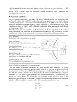
3.1 Inertial position control
We start the outer-loop feedback control design by transforming the tracking control
problem into a regulation problem:

()
01
ref
002 0
03
cos sin 0
sin cos 0
001
z
Zz XY
z
χχ
χχ
⎡⎤⎡ ⎤
⎢⎥⎢ ⎥
==− −
⎢⎥⎢ ⎥
⎢⎥⎢ ⎥
⎣⎦⎣ ⎦
(9)

where we introduce a vehicle carried vertical reference frame with origin in the center of
gravity and X-axis aligned with the horizontal component of the velocity vector (Ren and
Beard, 2004, Proud et al., 1999). Differentiating Eq. (9) now gives

(
)
()
ref ref
02
ref ref
001
ref
cos
sin
sin
Vz V
ZzV
zV
χχχ
χχχ
γ
⎡
⎤
+− −
⎢
⎥
⎢
⎥
=− + −
⎢
⎥
⎢
⎥

−
⎣
⎦




(10)

We want to control the position errors
0
Z
through the flight-path angles
χ
and
γ
, and the
total airspeed V. However, from Eq. (10) it is clear that it is not yet possible to do something
about
02
z
in this design step. Now we select the virtual controls

(
)
des,0 ref ref
01 01
cosVV cz
χχ
=−− (11)

ref
des,0
03 03
arcsin ,
22
cz z
V
π
π
γγ
⎛⎞
−
=
−<<
⎜⎟
⎝⎠

(12)

where
01
0c > and
03
0c > are the control gains. The actual implementable virtual control
signals
des
V
and
des

γ
, as well as their derivatives,
des
V

and
des
γ

, are obtained by filtering the
virtual signals with a second-order low-pass filter. In this way, tedious calculation of the
virtual control derivatives is avoided (Swaroop et al., 1997). An additional advantage is that
the filters can be used to enforce magnitude or rate limits on the states (Farrell et al., 2003,
2007). As an example, the state-space representation of such a filter for
des,0
V
is given by

()
()
()
2
1
2
des,0
212
2
2
V
VV R M

VV
q
qt
qt S S V q q
ω
ζω
ζω
⎡
⎤
⎡⎤
⎢
⎥
⎛⎞
=
⎛⎞
⎢⎥
⎢
⎥
⎡⎤
−−
⎜⎟
⎜⎟
⎢⎥
⎢
⎥
⎣⎦
⎜⎟
⎣⎦
⎜⎟
⎝⎠

⎢
⎥
⎝⎠
⎣
⎦


(13)

des
1
des
2
V
q
q
V
⎡⎤
⎡
⎤
=
⎢⎥
⎢
⎥
⎢⎥
⎣
⎦
⎣⎦

(14)

where
(
)
M
S ⋅ and
(
)
R
S
⋅
represent the magnitude and rate limit functions as given in (Farrell
et al., 2007). These functions enforce the state V to stay within the defined limits. Note that if
Advances in Flight Control Systems

28
the signal
des,0
V is bounded, then
des
V and
des
V

are also bounded and continuous signals.
When the magnitude and rate limits are not in effect, the transfer function from
des,0
V to
des
V is given by

des 2
des,0 2 2
2
V
VV V
V
Vs
ω
ζ
ωω
=
++
(15)
and the error
des,0 des
VV− can be made arbitrarily small by selecting the bandwidth of the
filter to be sufficiently large (Swaroop et al., 1997).
3.2 Flight-path angle and airspeed control
In this loop the objective is to steerV and
γ
to their desired values, as determined in the
previous section. Furthermore, the heading angle
χ
has to track the reference signal
ref
χ
, and
we also have to guarantee that
02
z is regulated to zero. The available (virtual) controls in this

step are the aerodynamic angles
μ
and
α
, as well as the thrust T . The lift, drag, and side
forces are assumed to be unknown and will be estimated. Note that the aerodynamic forces
also depend on the control-surface deflections
T
ear
U
δδδ
=
⎡
⎤
⎣
⎦
. These forces are quite
small, because the surfaces are primarily moment generators. However, because the current
control-surface deflections are available from the command filters used in the inner loop, we
can still take them into account in the control design. The relevant equations of motion are
given by

(
)
(
)
(
)
111 11 2 1
,,,XAFXUBGXUX HX=+ +


(16)
where
11 1
0 0 sin cos cos 0 0
1 cos 1 1
0 0 , cos sin cos , 0 0
cos cos cos
0sin 0 0 0 1
cos sin sin cos
Vg V
T
AH B
mV mV mV
g
T
mV V
γαβ
μ
αβμ
γγ γ
μ
αβμ γ
⎡⎤
⎢⎥
⎡⎤ ⎡ ⎤
−−
⎢⎥
⎢⎥ ⎢ ⎥
⎢⎥

⎢⎥ ⎢ ⎥
== =
⎢⎥
⎢⎥ ⎢ ⎥
⎢⎥
⎢⎥ ⎢ ⎥
−
⎢⎥
⎣⎦ ⎣ ⎦
−
⎢⎥
⎣⎦


are known (matrix and vector) functions, and
()
()
()
()
()
()
()
11
,
,, , sinsin
,
,sincos
T
LXU
F Y XU G L XU T

DXU
LXU T
α
μ
α
μ
⎡
⎤
⎡⎤
⎢
⎥
⎢⎥
⎢
⎥
==−
⎢⎥
⎢
⎥
⎢⎥
⎢
⎥
⎣⎦
−
⎣
⎦


are functions containing the uncertain aerodynamic forces. Note that the intermediate
control variables
α

and
μ
do not appear affine in the
1
X subsystem, which complicates the
design somewhat. Because the control objective in this step is to track the smooth reference
signal
(
)
des des des des
1
T
XV
χγ
= with
()
1
T
XV
χ
γ
= , the tracking errors are defined as
Adaptive Backstepping Flight Control for Modern Fighter Aircraft

29

11
des
112 11
13

z
Zz XX
z
⎡⎤
⎢⎥
==−
⎢⎥
⎢⎥
⎣⎦
(17)
To regulate
1
Z and
02
z to zero, the following equation needs to be satisfied (Kanayama et al.,
1990):

()
()
11 11
ref des
11 2 0202 12 12 11 1 1
13 13
ˆ
ˆ
,, sin
cz
BG X U X V c z c z AF H X
cz
−

⎡⎤
⎢⎥
=− + − − +
⎢⎥
⎢⎥
−
⎣⎦

(18)
where
1
ˆ
F
is the estimate of
1
F and

( ) ()()
()
()()
()
120
0
ˆ
ˆˆ
,, , , sin sin
ˆˆ
,,sincos
T
GXUX LXU L XU T

LXU LXU T
α
α
α
αμ
α
αμ
⎡
⎤
⎢
⎥
⎢
⎥
=++
⎢
⎥
⎢
⎥
++
⎢
⎥
⎣
⎦
(19)
with the estimate of the lift force decomposed as
()()()
0
ˆˆ ˆ
,,,LXU L XU L XU
α

α
=+
The estimate of the aerodynamic forces
1
ˆ
F
is defined as

()
11
1
ˆ
ˆ
,
T
FF
FXU
=
ΦΘ (20)
where
1
T
F
Φ is a known (chosen) regressor function and
1
ˆ
F
Θ
is a vector with unknown constant
parameters. It is assumed that there exists a vector

1
F
Θ
such that

(
)
11
1
,
T
FF
FXU
=
ΦΘ (21)

This means the estimation error can be defined as
111
ˆ
FFF
Θ
=Θ −Θ

. We now need to determine
the desired values
des
α
and
des
μ

. The right-hand side of Eq. (18) is entirely known, and so the
left-hand side can be determined and the desired values can be extracted. This is done by
introducing the coordinate transformation

()()
(
)
0
ˆˆ
,,sincosxLXULXU T
α
α
αμ
≡+ + (22)

()()
(
)
0
ˆˆ
,,sinsinyLXULXU T
α
α
αμ
≡+ + (23)

which can be seen as a transformation from the two-dimensional polar coordinates
()()
0
ˆˆ

,,sinLXU LXU T
α
α
α
++
and
μ
to Cartesian coordinates x and y. The desired signals
,0
00
T
des
Tyx
⎡
⎤
⎣
⎦
are given by
Advances in Flight Control Systems

30

()
des ,0
11 11
ref des
1 0 02 02 12 12 1 1 1 1
01313
ˆ
sin

Tcz
B
y
Vcz c z AFHX
xcz
⎡⎤
−
⎡⎤
⎢⎥
⎢⎥
=− + − − +
⎢⎥
⎢⎥
⎢⎥
⎢⎥
−
⎣⎦
⎣⎦

(24)
Thus, the virtual control signals are equal to

() ()
des,0 2 2
00 0
ˆˆ
,,sinLXU x y LXU T
α
α
α

=+− − (25)
and

(
)
()
()
00 0
00 0 0
des,0
00 0 0
00
00
arctan / if 0
arctan / if 0 and 0
arctan / if 0 and 0
/2 if 0 and 0
/2 if 0 and 0
yx x
yx x y
yx x y
xy
xy
π
μ
π
π
π
⎧
>

⎪
+
<≥
⎪
⎪
=
−
<<
⎨
⎪
=
>
⎪
⎪
−
=<
⎩
(26)
Filtering the virtual signals to account for magnitude, rate, and bandwidth limits will give
the implementable virtual controls
des
α
,
des
μ
and their derivatives. The sideslip-angle
command was already defined as
ref
0
β

=
, and thus
des des des
2
0
T
X
μα
⎡
⎤
=
⎣
⎦
and its derivative
are completely defined. However, care must be taken because the desired virtual control
des,0
μ
is undefined when both
0
x and
0
y
are equal to zero, making the system momentarily
uncontrollable. This sign change of
()()
0
ˆˆ
,,sinLXU LXU T
α
α

α
++can only occur at very low
or negative angles of attack. This situation was not encountered during the maneuvers
simulated in this study. To solve the problem altogether, the designer could measure the
rate of change for
0
x and
0
y
and devise a rule base set to change sign when these terms
approach zero. Furthermore, problems will also occur at high angles of attack when the
control effectiveness term
ˆ
L
α
will become smaller and eventually change sign. Possible
solutions include limiting the angle-of-attack commands using the command filters or
proper trajectory planning to avoid high-angle-of-attack maneuvers. Also note that so far in
the control design process, we have not taken care of the update laws for the uncertain
aerodynamic forces; they will be dealt with when the static control design is finalized.
3.3 Aerodynamic angle control
Now the reference signal
des des des des
2
[]
T
X
μαβ
= and its derivative have been found and
we can move on to the next feedback loop. The available virtual controls in this step are the

angular rates
3
X . The relevant equations of motion for this part of the design are given by

(
)
(
)
(
)
221 2 32
,XAFXUBXXHX=++

(27)
where
2 2
cos sin
0
tan tan sin tan cos 0
cos cos
11
0 0 , cos tan 1 sin tan
cos
sin 0 cos
010
AB
mV
αα
βγμγμ
ββ

α
βαβ
β
αα
⎡
⎤
⎡⎤
+
⎢
⎥
⎢⎥
⎢
⎥
−
⎢⎥
==−−
⎢
⎥
⎢⎥
⎢
⎥
⎢⎥
⎢
⎥
⎣⎦
⎢
⎥
⎣
⎦

Adaptive Backstepping Flight Control for Modern Fighter Aircraft

31
()
2
sin tan sin sin tan cos sin tan cos tan cos cos
1sin
cos cos
cos
cos cos cos sin
g
T
V
g
HT
mV V
g
T
V
α
γμ αβ αβγμ βγμ
α
γμ
β
αβ γμ
⎡ ⎤
+− −
⎢ ⎥
⎢ ⎥
⎢ ⎥

=+
⎢ ⎥
⎢ ⎥
⎢ ⎥
−+
⎢ ⎥
⎣ ⎦


are known (matrix and vector) functions. The tracking errors are defined as

des
222
ZXX=− (28)
To stabilize the
2
Z subsystem, a virtual feedback control
des,0
3
X is defined as

des,0 des
23 22 21 2 2 2 2
ˆ
,0
T
BX CZ AF H X C C
=
−−−+ =>


(29)

The implementable virtual control (i.e., the reference signal for the inner loop)
des
3
X and its
derivative are again obtained by filtering the virtual control signal
des,0
3
X with a second-order
command-limiting filter.
3.4 Angular rate control
In the fourth step, an inner-loop feedback loop for the control of the body-axis angular rates
3
T
X
pq
r=
⎡⎤
⎣⎦
is constructed. The control inputs for the inner loop are the control-surface
deflections
T
ear
U
δδδ
=
⎡⎤
⎣⎦
. The dynamics of the angular rates can be written as

()
()
(
)
()
333 3 3
,XAFXUBXUHX=++

(30)
where
(
)
()
()
12
34
22
37 356
49
82
0
00,
0
cr cp q
cc
Ac Hcprcpr
cc
cp cr q
⎡

⎤
+
⎡⎤
⎢
⎥
⎢⎥
==−−
⎢
⎥
⎢⎥
⎢
⎥
⎢⎥
−
⎣⎦
⎢
⎥
⎣
⎦

are known (matrix and vector) functions, and
0
303
0
,
ear
ear
ear
LLLL
FM BMMM

NNNN
δδδ
δδδ
δδδ
⎡
⎤⎡ ⎤
⎢
⎥⎢ ⎥
==
⎢
⎥⎢ ⎥
⎢
⎥⎢ ⎥
⎢
⎥⎢ ⎥
⎣
⎦⎣ ⎦

are unknown (matrix and vector) functions that have to be approximated. Note that for a
more convenient presentation, the aerodynamic moments have been decomposed: for
example,

(
)
(
)
0
,,
ear
ear

MXU M XU M M M
δδδ
δ
δδ
=+++ (31)
Advances in Flight Control Systems

32
where the higher-order control-surface dependencies are still contained in
(
)
0
,
M
XU . The
control objective in this feedback loop is to track the reference signal
des ref ref ref
3
[]
T
Xpqr=
with the angular rates
3
X . Defining the tracking errors

des
333
ZXX=− (32)
and taking the derivatives results in

()
()
(
)
()
des
333 3 3 3
,ZAFXUBXUHXX=++−

(33)

To stabilize the system of Eq. (33), we define the desired control
0
U as

0des
33 3 3 33 3 3 3 3
ˆˆ
,0
T
ABU CZ AF H X C C
=
−−−+ =>

(34)

where
3
ˆ
F

and
3
ˆ
B
are the estimates of the unknown nonlinear aerodynamic moment functions
3
F and
3
B , respectively. The F-16 model is not over-actuated (i.e., the
3
B matrix is square). If
this is not the case, some form of control allocation would be required (Enns, 1998, Durham,
1993). The estimates are defined as

()
()
33 33
33
ˆˆ
ˆˆ
,, ,for1,,3
i
ii
TT
FF BB
FXUB X i=Φ Θ =Φ Θ = " (35)

where
3
T

F
Φ and
3
i
T
B
Φ
are the known regressor functions,
3
ˆ
F
Θ
and
3
ˆ
i
B
Θ
are vectors with
unknown constant parameters, and
3
ˆ
i
B represents the ith column of
3
ˆ
B
. It is assumed that
there exist vectors
3

F
Θ
and
3
i
B
Θ
such that

(
)
(
)
33 33
33
,,
i
ii
TT
FF BB
FXUB X
=
ΦΘ=ΦΘ (36)

This means that the estimation errors can be defined as
333
ˆ
FFF
Θ
=Θ −Θ


and
333
ˆ
iii
BBB
Θ
=Θ −Θ

.
The actual controlU is found by applying a filter similar to Eq. (13) to
0
U .
3.5 Update laws and stability properties
We have now finished the static part of our control design. In this section the stability
properties of the control law are discussed and dynamic update laws for the unknown
parameters are derived. Define the control Lyapunov function

()()
()
()
11 1 33 3 3 3 3
22
12
00 11 13 22 33
02
3
11 1
1
122cos

2
1
trace trace trace
2
ii i
TTT
TT T
FF F FF F B B B
i
z
VZZz zZZZZ
c
−− −
=
⎛⎞
−
=++ ++++
⎜⎟
⎜⎟
⎝⎠
+ ΘΓΘ + ΘΓΘ + Θ Γ Θ
∑
   
(37)

with the update gains matrices
11 33
0, 0
TT
FF FF

Γ
=Γ > Γ =Γ > , and
33
0
ii
T
BB
Γ
=Γ > . Taking the
derivative ofV along the trajectories of the closed-loop system gives
Adaptive Backstepping Flight Control for Modern Fighter Aircraft

33
(
)
(
)
(
)
() ()
()
(
)
()
()
()
11
1
2des,0 ref2des,0
01 01 02 01 01 02 01 12 03 03 03

2ref 2 2
12
11 11 12 02 12 13 13 1 1 1 1 2 1 2
02
des,0
1112 12 222 22
sin sin sin
ˆ
sin sin
ˆˆ
TT
FF
TTT
F
Vczzz VV zzz V z czV z
c
cz V zz z cz Z A BG X G X
c
ZB G X G X ZCZ ZA
χχ γγ
=− + + − + − + − − − +
⎛⎞
−− + −+ ΦΘ+ − +
⎜⎟
⎜⎟
⎝⎠
+−−+Φ




()
()
1
33 3 3 11 1 33 3
33 3
des,0
22 3 3 3 33
3
01 1
33 333
1
3
1
1
ˆ
ˆˆ
trace trace
ˆ
trace
ii
ii i
TT T
F
TT T T T T
FF B B i FFF FFF
i
T
BB B
i
ZB X X ZCZ

ZA U ZAB U U
−−
=
−
=
Θ+ − − +
⎛⎞
⎛⎞⎛⎞
+ ΦΘ + Φ Θ + − − ΘΓΘ − ΘΓΘ +
⎜⎟⎜⎟
⎜⎟
⎝⎠⎝⎠
⎝⎠
⎛⎞
−ΘΓΘ
⎜⎟
⎝⎠
∑
∑


  


(38)
To cancel the terms in Eq. (38), depending on the estimation errors, we select the update
laws

()
(

)
111 333 3 333
1 1 22 33 33
ˆˆˆ
,,proj
iiii
TT T T
FFFa FFF B BBB i
A Z AZ AZ AZUΘ=ΓΦ + Θ=ΓΦ Θ = ΓΦ

(39)
with
() ()
(
)
11 11
1111212
ˆ
TT
aF F F F
AABGXGXΦΘ = ΦΘ + −


The update laws for
3
ˆ
B
include a projection operator (Ioannou and Sun, 1995) to ensure that
certain elements of the matrix do not change sign and full rank is maintained always. For
most elements, the sign is known based on physical principles. Substituting the update laws

in Eq. (38) leads to
()
()
()
()
()
()()
222ref 2 2 des,0
12
01 01 03 03 11 11 12 13 13 2 2 2 3 3 3 01
02
des,0 des,0 des,0 0
03 11 1 2 1 2 22 3 3 3 33
sin
ˆ
ˆ
sin sin
TT
TTT
c
Vczczcz V zczZCZZCZVV z
c
V z ZBGX GX ZBX X ZABUU
γγ
=−−−−− −− − +− +
−− + − + −+ −

(40)
where the first line is already negative semi-definite, which we need to prove stability in the
sense of Lyapunov. Because our Lyapunov function V equation (37) is not radially

unbounded, we can only guarantee local asymptotic stability (Kanayama et al., 1990). This is
sufficient for our operating area if we properly initialize the control law to
ensure
12
/2z
π
≤± . However, we also have indefinite error terms due to the tracking errors
and due to the command filters used in the design. As mentioned before, when no rate or
magnitude limits are in effect, the difference between the input and output of the filters can
be made small by selecting the bandwidth of the filters to be sufficiently larger than the
bandwidth of the input signal. Also, when no limits are in effect and the small bounded
difference between the input and output of the command filters is neglected, the feedback
controller designed in the previous sections will converge the tracking errors to zero (for
proof, see (Farrell et al., 2005, Sonneveldt et al., 2007, Yip, 1997)).
Naturally, when control or state limits are in effect, the system will in general not track the
reference signal asymptotically. A problem with adaptive control is that this can lead to
corruption of the parameter-estimation process, because the tracking errors that are driving
this process are no longer caused by the function approximation errors alone (Farrell et al.,
2003). To solve this problem we will use a modified definition of the tracking errors in the
update laws in which the effect of the magnitude and rate limits has been removed, as
suggested in (Farrell et al., 2005, Sonneveldt et al., 2006). Define the modified tracking errors
Advances in Flight Control Systems

34

111 222 333
,,ZZ ZZ ZZ
=
−Ξ = −Ξ = −Ξ


(41)
with the linear filters

()
(
)
(
)
()
()
des,0
11111 21 2
des,0
222233
0
33333
ˆˆ
,, ,,
ˆ
CBGXUXGXUX
CBXX
CABUU
Ξ=− Ξ+ −
Ξ=− Ξ+ −
Ξ=− Ξ+ −



(42)
The modified errors will still converge to zero when the constraints are in effect, which

means the robustified update laws look like

()
(
)
111 333 3 333
1 1 22 33 33
ˆˆˆ
,,proj
iiii
TT T T
FFFa FFF B BBB i
A Z AZ AZ AZUΘ=ΓΦ + Θ=ΓΦ Θ = ΓΦ

(43)
To better illustrate the structure of the control system, a scheme of the adaptive inner-loop
controller is shown in Fig. 2.
4. Model identification
To simplify the approximation of the unknown aerodynamic force and moment functions,
thereby reducing computational load, the flight envelope is partitioned into multiple
connecting operating regions called hyperboxes or clusters. This can be done manually
using a priori knowledge of the nonlinearity of the system, automatically using nonlinear
optimization algorithms that cluster the data into hyperplanar or hyperellipsoidal clusters
(Babuška, 1998) or a combination of both. In each hyperbox a locally valid linear-in-the-
parameters nonlinear model is defined, which can be estimated using the update laws of the
Lyapunov-based control laws. The aerodynamic model can be partitioned using different
state variables, the choice of which depends on the expected nonlinearities of the system. In
this study we use B-spline neural networks (Cheng et al., 1999, Ward et al., 2003) (i.e., radial
basis function neural networks with B-spline basis functions) to interpolate between the
local nonlinear models, ensuring smooth transitions. In the previous section we defined

parameter update laws equation (43) for the unknown aerodynamic functions, which were
written as

() ()
()
11 33 33
13 3
ˆˆˆ
ˆˆˆ
,, ,,
i
ii
TT T
FF FF BB
FXUFXUB X
=
ΦΘ=ΦΘ=ΦΘ (44)
Now we will further define these unknown vectors and known regressor vectors. The total
force approximations are defined as

() ( )
()
()
()() () () ()
()()
()
0
0
0
ˆˆ ˆ ˆ

ˆ
,, ,
2
ˆˆ ˆ ˆ ˆ ˆ
,, , , , ,
22
ˆˆ
ˆ
,, ,
q
e
pr
ar
e
LLeL Le
YeY Y Y aY r
DeD e
qc
LqSC C C C
V
pb
rb
YqSC C C C C
VV
DqSC C
αδ
δδ
δ
αβ βδ α α αβδ
α

βδ αβ αβ αβδ αβδ
αβδ αβδ
⎛⎞
=+++
⎜⎟
⎝⎠
⎛⎞
=++++
⎜⎟
⎝⎠
=+
(45)
Adaptive Backstepping Flight Control for Modern Fighter Aircraft

35

Fig. 2. Inner-loop control system
and the moment approximations are defined as
()() () () () ()
()
()
()
()() () () () ()
0
0
0
ˆ
ˆˆ ˆ ˆˆˆ
,, , , , , ,
22

ˆ
ˆˆ ˆ
,,
2
ˆ
ˆˆ ˆ ˆˆˆ
,, , , , , ,
22
pr
ear
q
e
pr
ear
eear
LL L LLL
e
MM M
e ear
NN N NNN
pb
rb
LqSC C C C C C
VV
qc
MqSC C C
V
pb
rb
NqSC C C C C C

VV
δδδ
δ
δδδ
αβδ αβ αβ αβδ αβδ αβδ
αβ α αβδ
α
βδ αβ αβ αβδ αβδ αβδ
⎛ ⎞
=+++++
⎜ ⎟
⎝ ⎠
⎛⎞
=++
⎜⎟
⎝⎠
⎛ ⎞
=+++++
⎜ ⎟
⎝ ⎠
(46)
Note that these approximations do not account for asymmetric failures that will introduce
coupling of the longitudinal and lateral motions of the aircraft. If a failure occurs that
introduces a parameter dependency that is not included in the approximation, stability can
no longer be guaranteed. It is possible to include extra cross-coupling terms, but this is
beyond the scope of this paper. The total nonlinear function approximations are divided
into simpler linear-in-the parameter nonlinear coefficient approximations: for example,

() ()
0

00
ˆ
ˆ
,,
LL
T
LCC
C
α
βϕαβθ
= (47)
where the unknown parameter vector
0
ˆ
L
C
θ
contains the network weights (i.e., the unknown
parameters), and
0
L
C
ϕ
is a regressor vector containing the B-spline basis functions
(Sonneveldt et al., 2007). All other coefficient estimates are defined in similar fashion. In this
case a two-dimensional network is used with input nodes for
α
and
β
. Different scheduling

parameters can be selected for each unknown coefficient. In this study we used third-order
B-splines spaced 2.5 deg and one or more of the selected scheduling variables
α
,
β
and
e
δ
.
Following the notation of Eq. (47), we can write the estimates of the aerodynamic forces and
moments as

() () ()
() () ()
ˆ
ˆˆ
ˆˆ ˆ
,, , ,, , ,,
ˆˆ ˆ
ˆˆˆ
,, , ,, , ,,
TT T
LeL YeY DeD
TT T
eee
LLMMNN
LY D
LM N
αβδ αβδ αβδ
αβδ αβδ αβδ

=Φ Θ =Φ Θ =Φ Θ
=Φ Θ =Φ Θ =Φ Θ
(48)
Advances in Flight Control Systems

36
which is a notation equivalent to the one used in Eq. (44). Therefore, the update laws
equation (43) can indeed be used to adapt the B-spline network weights. In practice
nonparametric uncertainties such as 1) un-modeled structural vibrations 2) measurement
noise, 3) computational round-off errors and sampling delays, and 4) time variations of the
unknown parameters, can result in parameter drift. One approach to avoiding parameter
drift taken here is to stop the adaptation process when the training error is very small (i.e. a
dead zones (Babuška, 1998, Karason and Annaswamy, 1994)).
5. Simulation results
This section presents the simulation results from the application of the flight-path controller
developed in the previous sections to the high-fidelity, six-degree-of-freedom F-16 model of
Sec. 2. Both the control law and the aircraft model are written as C S-functions in
MATLAB/Simulink. The simulations are performed at three different starting flight
conditions with the trim conditions: 1) h= 5000 m, V= 200 m/s, and α=θ=2.774 deg; 2) h=0 m,
V =250 m/s, and α=θ=2.406 deg; and 3) h= 2500 m, V= 150 m/s, and α=θ=0.447 deg; where h
is the altitude of the aircraft, and all other trim states are equal to zero.
Furthermore, two maneuvers are considered: 1) a climbing helical path and 2) a
reconnaissance and surveillance maneuver. The latter maneuver involves turns in both
directions and some altitude changes. The simulations of both maneuvers last 300 s. The
reference trajectories are generated with second-order linear filters to ensure smooth
trajectories. To evaluate the effectiveness of the online model identification, all maneuvers
will also be performed with a ±30% deviation in all aerodynamic stability and control
derivatives used by the controller (i.e., it is assumed that the onboard model is very
inaccurate). Finally, the same maneuvers are also simulated with a lockup at ±10 deg of the
left aileron.

5.1 Control parameter tuning
We start with the selection of the gains of the static control law and the bandwidths of the
command filters. Lyapunov stability theory only requires the control gains to be larger than
zero, but it is natural to select the largest gains of the inner loop. Larger gains will, of course,
result in smaller tracking errors, but at the cost of more control effort. It is possible to derive
certain performance bounds that can serve as guidelines for tuning (see, for example, Krstić,
et al., 1993, Sonneveldt et al., 2007). However, getting the desired closed-loop response is
still an extensive trial-and-error procedure. The control gains were selected as
01
0.1c = ,
5
02
10c
−
= ,
03
0.5c =
,
11
0.01c =
,
12
2.5c =
,
13
0.5c =
,
(
)
2

dia
g
1,1,1C = ,
()
3
dia
g
2,2,2C = .
The bandwidths of the command filters for the actual control variables
e
δ
,
a
δ
, and
r
δ
are
chosen to be equal to the bandwidths of the actuators, which are given in (Sonneveldt et al.,
2007). The outer-loop filters have the smallest bandwidths. The selection of the other
bandwidths is again trial and error. A higher bandwidth in a certain feedback loop will
result in more aggressive commands to the next feedback loop. All damping ratios are equal
to 1.0. It is possible to add magnitude and rate limits to each of the filters. In this study
magnitude limits on the aerodynamic roll angle
μ
and the flight-path angle
γ
are used to
avoid singularities in the control laws. Rate and magnitude limits equal to those of the
actuators are enforced on the actual control variables.

Adaptive Backstepping Flight Control for Modern Fighter Aircraft

37
The selected command-filter parameters can be found back in Table 1. As soon as the
controller gains and command-filter parameters have been defined, the update law gains
can be selected. Again, the theory only requires that the gains should be larger than zero.
Larger update gains means higher learning rates and thus more rapid changes in the B-
spline network weights.
5.2 Manoeuvre 1: upward spiral
In this section the results of the numerical simulations of the first test maneuver, the
climbing helical path, are discussed. For each of the three flight conditions, five cases are
considered: nominal, the aerodynamic stability and control derivatives used in the control law
perturbed with +30% and with -30% with respect to the real values of the model, a lockup of
the left aileron at +10 deg, and a lockup at -10 deg. No actuator sensor information is used. In
Fig. 3 the results are plotted of the simulation without uncertainty, starting at flight condition
1. The maneuver involves a climbing spiral to the left with an increase in airspeed. It can be
seen that the control law manages to track the reference signal very well and closed-loop
tracking is achieved. The sideslip angle does not become any larger than ±0.02 deg. The
aerodynamic roll angle does reach the limit set by the command filter, but this has no
consequences for the performance. The use of dead zones ensures that the parameter update
laws are indeed not updating during this maneuver without any uncertainties. The responses
at the two other flight conditions are virtually the same, although less thrust is needed due to
the lower altitude of flight condition 2 and the lower airspeed of flight condition 3. The other
control surfaces are also more efficient. This is illustrated in Tables 2–4, in which the mean
absolute values (MAVs) of the outer-loop tracking errors, control-surface deflections, and
thrust can be found. Plots of the parameter-estimation errors are not included. However, the
errors converge to constant values, but not to zero, as is common with Lyapunov-based
update laws (Sonneveldt et al., 2007, Page and Steinberg, 1999).

Table 1. Command-filter parameters


Table 2. Manoeuvre 1 at flight condition 1: mean absolute value of tracking errors and
control inputs
Advances in Flight Control Systems

38

Table 3. Manoeuvre 1 at flight condition 2: mean absolute value of tracking errors and
control inputs



Table 4. Manoeuvre 1 at flight condition 3: mean absolute value of tracking errors and
control inputs
The response of the closed-loop system during the same maneuver starting at flight
condition 1, but with +30% uncertainties in the aerodynamic coefficients, is shown in Fig. 4.
It can be observed that the tracking errors of the outer loop are now much larger, but in the
end, the steady-state tracking error converges to zero. The sideslip angle still remains within
0.02 deg. Some small oscillations are visible in Fig. 4j, but these stay well within the rate and
magnitude limits of the actuators. In Tables 2–4 the MAVs of the tracking errors and control
inputs are shown for all flight conditions. As was already seen in the plots, the average
tracking errors increase, but the magnitude of the control inputs stays approximately the
same. The same simulations have been performed for a -30% perturbation in the stability
and control derivatives used by the control law, and the results are also shown in the tables.
It appears that underestimated initial values of the unknown parameters lead to larger
tracking errors than overestimates for this maneuver. Finally, the maneuver is performed
with the left aileron locked at ±10 deg [i.e.,
(

)
damaged
0.5 10 /180
aa
δδπ
=± ]. Figure 5 shows the
response at flight condition 3 with the aileron locked at -10 deg.
Except for some small oscillations in the response of roll rate p, there is no real change in
performance visible; this is confirmed by the numbers of Table 4. However, from Tables 2
and 3 we observe that aileron and rudder deflections become larger with both locked aileron
failure cases, whereas tracking performance hardly declines.
5.3 Manoeuvre 2: reconnaissance
The second maneuver, called reconnaissance and surveillance, involves turns in both
directions and altitude changes, but airspeed is kept constant. Plots of the simulation at
flight condition 3 with -30% uncertainties are shown in Fig. 6. Tracking performance is again
excellent and the steady-state tracking errors converge to zero. There are some small
oscillations in the rudder deflection, but these are within the limits of the actuator. We
compare the MAVs of the tracking errors and control inputs with those for the nominal case
in Table 5 and observe that the average tracking errors have not increased much for this
case. The degradation of performance for the uncertainty cases is somewhat worse at the
other two flight conditions, as can be seen in Tables 6 and 7. The sideslip angle always
remains within 0.05 deg for all flight conditions and uncertainties. Corresponding with the
Adaptive Backstepping Flight Control for Modern Fighter Aircraft

39
results of maneuver 1, overestimation of the unknown parameters again leads to smaller
tracking errors. Simulations of maneuver 2 with the locked aileron are also performed.
Figure 7 shows the results for flight condition 1 with a locked aileron at _10 deg. Some very
small oscillations are again visible in the roll rate, aileron, and rudder responses, but
tracking performance is good and steady-state convergence is achieved.

Table 6 confirms that the results of the simulations with actuator failure hardly differ from
the nominal case. There is only a small increase in the use of the lateral control surfaces. The
same holds at the other flight conditions, as can be seen in Tables 5 and 7.


Table 5. Manoeuvre 2 at flight condition 3: mean absolute value of tracking errors and
control inputs


Table 6. Manoeuvre 2 at flight condition 1: mean absolute value of tracking errors and
control inputs


Table 7. Manoeuvre 2 at flight condition 2: mean absolute value of tracking errors and
control inputs
6. Conclusions
In this paper a nonlinear adaptive flight-path control system is designed for a high-fidelity
F-16 model. The controller is based on a backstepping approach with four feedback loops
that are designed using a single control Lyapunov function to guarantee stability. The
uncertain aerodynamic forces and moments of the aircraft are approximated online with B-
spline neural networks for which the weights are adapted by Lyapunov-based update laws.
Numerical simulations of two test maneuvers were performed at several flight conditions to
verify the performance of the control law. Actuator failures and uncertainties in the stability
and control derivatives are introduced to evaluate the parameter-estimation process. The
results show that trajectory control can still be accomplished with these uncertainties and
failures, and good tracking performance is maintained. Compared with other Lyapunov-
Advances in Flight Control Systems

40
based trajectory control designs, the present approach is much simpler to apply and the

online estimation process is more robust to saturation effects. Future studies will focus on
the actual trajectory generation and the extension to formation-flying control.
Appendix constraint adaptive backstepping
Backstepping [21] is a systematic, Lyapunov-based method for nonlinear control design,
which can be applied to nonlinear systems that can be transformed into lower-triangular
form, such as the system of Eq. (A.1):

(
)
(
)
11 12
xfx gxx=+

(A.1)
The name “backstepping” refers to the recursive nature of the control law design procedure.
Using the backstepping procedure, a control law is recursively constructed, along with a
control Lyapunov function (CLF) to guarantee global stability. For the system Eq. (A.1), the
aim of the design procedure is to bring the state vector
1
x
to the origin. The first step is to
consider
2
x
as the virtual control of the scalar
1
x
subsystem and to find a desired virtual control
law

()
11
x
α
that stabilizes this subsystem by using the control Lyapunov function
(
)
11
Vx :

()
2
11 1
1
2
Vx x=
(A.2)
The time derivative of this CLF is negative definite

()
(
)
() () ()
11
11 1 1 11 1
1
0, 0
Vx
Vx fx gx x x
x

α
∂
⎡⎤
=
+<≠
⎣⎦
∂

(A.3)
If only the virtual control law

(
)
211
xx
α
= (A.4)
could be satisfied. The key property of backstepping is that we can now “step back” through
the system. If the error between
2
x and its desired value is defined as

(
)
211
zx x
α
=−
(A.5)
the system Eq. (6) can be rewritten in terms of this error state

(
)
(
)
(
)
()
() () ()
()
11 111
11
1111
1
xfx gx x z
x
zu fx gx x z
x
α
α
α
⎡⎤
=+ +
⎣⎦
∂
⎡
⎤
=− + +
⎣
⎦

∂


(A.6)
The control Lyapunov function Eq. (A.2) can now be expanded with a term penalizing the
error state
z


()
()
2
21 11
1
,
2
Vxz Vx z=+
(A.7)
Adaptive Backstepping Flight Control for Modern Fighter Aircraft

41
In simplified notation the time derivative of
2
V is equal to

() ()
()
11
21 1
11

111
11
111
V
Vfgzzufgz
xx
VV
fg z gu fg z
xxx
α
αα
α
αα
⎛⎞
∂∂
⎡
⎤⎡⎤
=+++−++
⎜⎟
⎣
⎦⎣⎦
∂∂
⎝⎠
⎛⎞
∂∂∂
⎡
⎤
=++ +−++
⎡⎤
⎜⎟

⎣⎦
⎣
⎦
∂∂∂
⎝⎠

(A.8)
which can be rendered negative definite with the control law

()
11
1
11
,0
V
ucz fg z gc
xx
α
α
∂∂
⎡⎤
=
−+ + + − >
⎣⎦
∂∂
(A.9)
This design procedure can also be used for a system with a chain of integrators. The only
difference is that there will be more virtual states to “backstep” through. Starting with the
state “farthest” from the actual control, each step of the backstepping technique can be
broken up into three parts: 1. Introduce a virtual control

1
α
and an error state z , and rewrite
the current state equation in terms of these; 2. choose a CLF for the system, treating it as a
final stage; 3) choose an equation for the virtual control that makes the CLF stabilizable.
The CLF is augmented at subsequent steps to reflect the presence of new virtual states, but
the same three stages are followed at each step. Hence, backstepping is a recursive design
procedure.
For systems with parametric uncertainties there exists a method called adaptive
backstepping (Kannelakopoulos et al., 1991), which achieves boundedness of the closed-
loop states and convergence of the tracking error to zero.
Consider the parametric strict-feedback system

(
)
()
() ()
1211
1111
,,
T
T
nnn n
T
nn
xxx
xxxx
xxux
−−−
=+

=+
=+

## #

"

ϕθ
ϕ
θ
βϕθ
(A.10)
where
(
)
0x
β
≠ for all
n
x ∈ \ ,
θ
is a vector of unknown constant parameters, and
i
ϕ
are
known (smooth) function vectors. The control objective is to asymptotically track a given
reference
()
r
y

t
with
1
x . All derivatives of
(
)
r
y
t
are assumed to be known.
The adaptive backstepping design procedure is similar to the normal backstepping
procedure, only this time a control law (static part) and a
parameter update law (dynamic
part) are designed along with a control Lyapunov function to guarantee global stability. The
control law makes use of a parameter estimate
ˆ
θ
, which is constantly adapted by the
dynamic parameter update law. Furthermore, the control Lyapunov function now contains
an extra term that penalizes the parameter estimation error
ˆ
θ
θθ
=
−

.
Theorem A.1 (Adaptive Backstepping Method): To stabilize the system Eq. (A.9) an error
variable is introduced for each state

()
1
1
i
iir i
zxy
α
−
−
=− − (A.11)
along with a virtual control law
Advances in Flight Control Systems

42
()
()
()
()
11
1
11 1 1
11
1
12
ˆˆ
,,
ˆˆ
ii
i k
T

ii i i
ii r ii i i k r i ik
k
kk
k
r
x
y
cz z x
y
z
x
y
−−
−
−− − −
−+
−
==
⎛⎞
∂∂ ∂ ∂
=− − − + + + Γ + Γ
⎜⎟
⎜⎟
∂
∂∂
∂
⎝⎠
∑∑
αα α α

α
θωθ τω
θθ
(A.12)
for
1,2, ,in= " , where the tuning function
i
τ
and the regressor vectors
i
ω
are defined as

()
(
)
1
1
ˆ
,,
i
ii r i ii
x
y
z
τ
θτω
−
−
=+ (A.13)

and

()
()
1
2
1
1
ˆ
,,
i
i
i
ii r i k
k
k
xy
x
−
−
−
=
∂
=−
∂
∑
α
ω
θϕ ϕ
(A.14)

where
(
)
12
,,,
ii
xxx x= " ,
() ()
(
)
,,,
ii
rirr r
y
yy y=

"
. 0
i
c > are design constants. With these new
variables the control and adaptation laws can be defined as

()
()
(
)
()
1
1
ˆ

,,
nn
nr r
uxyy
x
αθ
β
−
⎡
⎤
=+
⎢
⎥
⎣
⎦
(A.15)
and

()
(
)
1
ˆˆ
,,
n
nr
xy Wz
θτθ
−
=Γ =Γ


(A.16)
where 0
T
Γ=Γ > is the adaptation gain matrix and W the regressor matrix

(
)
()
1
ˆ
,,,
i
Wz
θ
ωω
= " (A.17)
The control law Eq. (A.15) together with the update law Eq. (A.17) renders the derivative of
the Lyapunov function

21
1
11
22
n
T
i
i
Vz
θ

θ
−
=
=+Γ
∑

(A.18)
negative definite and thus this adaptive controller guarantees global boundedness of
()
xt
and asymptotically tracking of a given reference
(
)
r
y
t with
1
x .
Proof of this theorem can be found in Sec. 4.3 of (Krstić et al., 1992).
The standard adaptive backstepping procedure as has been discussed so far has a number of
drawbacks.
1.
The analytic calculation of the virtual control derivatives is tedious, especially for large
systems;
2.
The procedure can only handle systems that can be transformed into a lower-triangular
form;
3.
Constraints on the inputs and states are not taken into account.
The third drawback can be a major problem when designing for flight control, because the

actuators of an aircraft have rate, bandwidth, and magnitude constraints. When the control
signal demanded by the backstepping controller cannot be generated by the actuators, that
is, the actuators saturate, stability can no longer be guaranteed. The problem becomes worse

Adaptive Backstepping Flight Control for Modern Fighter Aircraft

43


Fig. 3. Manoeuvre 1: climbing helical path performed at flight condition 1 without any
uncertainty or actuator failures
Advances in Flight Control Systems

44



Fig. 4. Manoeuvre 1: climbing helical path performed at flight condition 2 with +30%
uncertainties in the aerodynamic coefficients
Adaptive Backstepping Flight Control for Modern Fighter Aircraft

45



Fig. 5. Manoeuvre 1: climbing helical path performed at flight condition 3 with left aileron
locked at -10 deg
Advances in Flight Control Systems

46

Fig. 6. Manoeuvre 2: reconnaissance and surveillance performance at flight condition 3 with
-30% uncertainties in the aerodynamic coefficients