Frontiers in Guided Wave Optics and Optoelectronics Part 3 pot
Bạn đang xem bản rút gọn của tài liệu. Xem và tải ngay bản đầy đủ của tài liệu tại đây (1.1 MB, 40 trang )
Irradiation Effects in Optical Fibers
65
systems for ITER, Proceedings of the 33rd EPS Conference on Plasma Phys., Rome, June
2006,
ITER Physics Expert Group on Diagnostics (1999). ITER Physics basis, Nucl. Fusion, Vol. 39,
(1999), (2541-2575)
Kaiser, P. (1974). Drawing-induced coloration in vitreous silica fibers, JOSA, Vol. 64, No. 4,
(1974), (475-481), ISSN doi:10.1364/JOSA.64.000475
Kajihara, K.; Hirano, M.; Skuja, L. & Hosono, H. (2008). Intrinsic defect formation in
amorphous SiO
2
by electronic excitation: Bond dissociation versus Frenkel
mechanisms, Physical Review B, Vol. 78, No.9 (September 2008), (094201 1-8), ISSN
1098-0121
Karlitschek, P.; Hillrichs, G. & Klein, K F. (1995). Photodegradation and nonlinear effects in
optical fibers induced by pulsed uv-laser radiation, Optics Communications, Vol. 116,
No. 1-3, (1995), (219-230), ISSN 0030-4018
Karlitschek, P.; Hillrichs, G. & Klein, K F. (1998). Influence of hydrogen on the colour center
formation in optical fibers induced by pulsed UV-laser radiation: Part 2: All-silica
fibers with low-OH undoped core, Optics Communications, Vol. 155, (October 1998)
(386-397), ISSN 0030-4018
Kimurai, E. Takada, Y. Hosono, M. Nakazawa, Takahashi, H. & Hayami, H. (2002). New
Techniques to Apply Optical Fiber Image Guide to Nuclear Facilities, J. of Nuclear
Sci. and Techn., Vol. 39, n
o
6, (603-607), ISSN 0022-3131
Li, J.; Lehman, R. L. & Sigel, G. H. Jr (1996). Electron paramagnetic resonance
characterization of nonuniform distribution of hydrogen in silica optical fibers,
Applied Physics Letters, Vol. 69, No. 14, (September 1996), (2131-2133), ISSN 0003-
6951
Mashkov, V. A.; Austin, Wm. R. ; Zhang, Lin & Leisure, R. G. (1996). Fundamental role of
creation and activation in radiation-induced defect production in high-purity
amorphous SiO
2
, Physical Review Letters, Vol. 76, No.16 (October 1995), (2926-2929),
ISSN 0031-9007
Messina, F.; Agnello S.; Cannas, M. & Parlato, A. (2009). Room temperature instability of E′
γ
centers induced by γ irradiation in Amorphous SiO
2
, The Journal of Physical
Chemistry A, Vol. 113, No.6, (December 2008), (1026-1032), ISSN 1520-5215
Nuccio, L.; Agnello, S. & Boscaino, R. (2009). Role of H
2
O in the thermal annealing of the E’
γ
center in amorphous silicon dioxide, Physical Review B, Vol. 79, N. 12, (March 2009),
(125205 1-8) ISSN 1098-0121
O'Keeffe, S.; Fitzpatrick, C.; Lewis, E. & Al-Shamma'a, A.I. (2008). A review of optical fibre
radiation dosimeters, Sensor Review, Vol. 28, No. 2, (136 – 142), ISSN 0260-2288
Ott, M.N. (2002). Radiation effects data on commercially available optical fiber: database
summary, Proceedings of 2002 IEEE Radiation Effects Data Workshop, pp. 24 – 31,
ISBN 0-7803-7544-0, Phoenix, July 2002, Institute of Electrical and Electronics
Engineers, Inc.
Pacchioni, G.; Skuja, L. & Griscom, D. L. (2000). Defects in SiO
2
and related dielectrics: science
and technology, Kluver Academic Publishers, ISBN 0-7923-6686-7, Dordrecht
Radiation effects, The 10 th Europhysical Conference on Defects in Insulation Materials,
Phys. Status Solidi, Vol. 4, No. 3 , (2007), (1060-1175)
Frontiers in Guided Wave Optics and Optoelectronics
66
Radzig, V. A. (1998). Point defects in disordered solids: Differences in structure and
reactivity of the (O≡Si-O)
2
Si: groups on silica surface, Journal of Non-Crystalline
Solids, Vol. 239, (1998), (49-56), ISSN 0022-3093
Reichle, R.; Brichard, B.; Escourbiac, F.; Gardarein, J.L.; Hernandez, D.; Le Niliot, C.;
Rigollet, F.; Serra, J.J.; Badie, J.M.; van Ierschot, S.; Jouve, M.; Martinez, S.; Ooms,
H.; Pocheau, C.; Rauber, X.; Sans, J.L.; Scheer, E.; Berghmans, F. & Decréton, M.
(2007). Experimental developments towards an ITER thermography diagnostic, J. of
Nuclear Materials, Vol. 363-365, (June 2007), (1466-1471),
doi:10.1016/j.jnucmat.2007.01.207
Shikama, T.; Nishitani, T.; Kakuta, T.; Yamamoto, S.; Kasai, S.; Narui, M.; Hodgson, E.;
Reichle, R.; Brichard, B.; Krassilinikov, A.; Snider, R.; Vayakis, G. & Costley A.
(2003). Irradiation test of diagnostic components for ITER application in a fission
reactor, Japan materials testing reactor, Nuclear fusion, Vol. 43, No. 7, (2003), (517-
521), ISSN 0029-5515
Skuja, L. (1998). Optically active oxygen-deficiency-related centers in amorphous silicon
dioxide, Journal of Non-Crystalline Solids, Vol. 239, No. 1-3, (1998), (16-48), ISSN
0022-3093
Skuja, L.; Hirano, M.; Hosono, H. & Kajihara, K. (2005). Defects in oxide glasses, Physica
Status Solidi (c), Vol. 2, No.1, (2005), (15-24), DOI:10.1002/pssc.200460102
Sporea D. & Sporea, R. (2005). Setup for the in situ monitoring of the irradiation-induced
effects in optical fibers in the ultraviolet-visible optical range, Review of Scientific
Instruments, Vol. 76, No. 11, (2005), DOI:10.1063/1.2130932
Sporea, D.; Sporea, A.; Agnello, S.; Nuccio, L.; Gelardi, F.M. & Brichard, B. (2007).
Evaluation of the UV optical transmission degradation of gamma-ray irradiated
optical fibers, CLEO/ The 7
th
Pacific Rim Conference on Lasers and Electro-Optics, Seoul,
August 2007
Troska, J.; Cervelli, G.; Faccio, F.; Gill, K.; Grabit, R.; Jareno, R.M.; Sandvik, A.M. & Vasey, F.
(2003). Optical readout and control systems for the CMS tracker, IEEE Trans.
Nuclear Sci., Vol. 50, No. 4, Part 1, (2003) (1067-1072), ISSN 0018-9499
Weeks, R.A. (1956). Paramagnetic resonance of lattice defects in irradiated quartz, J. Appl.
Phys., Vol. 27, No. 11, (1956), (1376-1381), DOI:10.1063/1.1722267
Weeks, R. A. & Sonder, E. (1963). The relation between the magnetic susceptibility, electron
spin resonance, and the optical absorption of the E
1
’center in fused silica, In:
Paramagnetic Resonance II, W. Low (Ed.), 869-879, Academic Press, LCCN 63-21409,
New York
Weil, J. A.; Bolton, J. R. & Wertz, J. E. (1994) Electron Paramagnetic Resonance, John Wiley &
Sons, 0-471-57234-9, New York
Zabezhailov, M.O.; Tomashuk, A.L.; Nikolin, I.V. & Plotnichenko, V.G. (2005). Radiation-
induced absorption in high-purity silica fiber preforms, Inorganic Materials, Vol. 41,
No.
3, (2005), (315–321), ISSN 0020-1685
4
Programmable All-Fiber Optical Pulse Shaping
Antonio Malacarne
1
, Saju Thomas
2
, Francesco Fresi
1,2
, Luca Potì
3
,
Antonella Bogoni
3
and Josè Azaña
2
1
Scuola Superiore Sant’Anna, Pisa,
2
Institut National de la Recherche Scientifique (INRS), Montreal, QC,
3
Consorzio Nazionale Interuniversitario per le Telecomunicazioni (CNIT), Pisa,
1,3
Italy
2
Canada
1. Introduction
Techniques for the precise synthesis and control of the temporal shape of optical pulses with
durations in the picosecond and sub-picosecond regimes have become increasingly
important for a wide range of applications in such diverse fields as ultrahigh-bit-rate optical
communications (Parmigiani et al., 2006; Petropoulos et al., 2001; Oxenlowe et al., 2007;
Otani et al., 2000), nonlinear optics (Parmigiani et al., 2006 b), coherent control of atomic and
molecular processes (Weiner, 1995) and generation of ultra-wideband RF signals (Lin &
Weiner, 2007). To give a few examples, (sub-)picosecond flat-top optical pulses are highly
desired for nonlinear optical switching (e.g. for improving the timing-jitter tolerance in
ultrahigh-speed optical time domain de-multiplexing (Parmigiani et al., 2006; Petropoulos et
al., 2001; Oxenlowe et al., 2007)) as well as for a range of wavelength conversion applications
(Otani et al., 2000); high-quality picosecond parabolic pulse shapes are also of great interest,
e.g. to achieve ultra-flat self-phase modulation (SPM)-induced spectral broadening in super-
continuum generation experiments (Parmigiani et al., 2006 b). For all these applications, the
shape of the synthesized pulse needs to be accurately controlled for achieving a minimum
intensity error over the temporal region of interest. The most commonly used technique for
arbitrary optical pulse shaping is based on spectral amplitude and/or phase linear filtering
of the original pulse in the spatial domain; this technique is usually referred to as ‘Fourier-
domain pulse shaping’ and has allowed the programmable synthesis of arbitrary waveforms
with resolutions better than 100fs (Weiner, 1995). Though extremely powerful and flexible,
the inherent experimental complexity of this implementation, which requires the use of very
high-quality bulk-optics components (high-quality diffraction gratings, high-resolution
spatial light modulators etc.), has motivated research on alternate, simpler solutions for
optical pulse shaping. This includes the use of integrated arrayed waveguide gratings
(AWGs) (Kurokawa et al., 1997), and fiber gratings (e.g. fiber Bragg gratings (Petropoulos et
al., 2001), or long period fiber gratings (Park et al. 2006)). However, AWG-based pulse
shapers (Kurokawa et al., 1997) are typically limited to time resolutions above 10ps. The
main drawback of the fiber grating approach (Petropoulos et al., 2001; Park et al. 2006) is the
lack of programmability: a grating device is designed to realize a single pulse shaping
operation over a specific input pulse (of prescribed wavelength and bandwidth) and once
Frontiers in Guided Wave Optics and Optoelectronics
68
the grating is fabricated, these specifications cannot be later modified. Recently, a simple
and practical pulse shaping technique using cascaded two-arm interferometers has been
reported (Park & Azaña, 2006). This technique can be implemented using widely accessible
bulk-optics components and can be easily reconfigured to synthesize a variety of transform-
limited temporal shapes of practical interest (e.g. flat-top and triangular pulses) as well as to
operate over a wide range of input bandwidths (in the sub-picosecond and picosecond
regimes) and center wavelengths. However, this solution presents all the drawbacks due to
a free-space solution where it is needful to strictly set the relative time delay inside each
interferometer in order to “program” different obtainable pulse shapes. Therefore the
pursuit of an integrated (fiber) pulse shaping solution, including full compatibility with
waveguide/fiber devices, which can be able to provide the additional functionality of
electronic programmability, manifests to be useful for a lot of different application fields.
For this reason a programmable fiber-based phase-only spectral filtering setup has been
recently introduced (Azaña et al., 2005; Wang & Wada, 2007). In the next section the
working principle of this spectral phase-only linear filtering approach is discussed and an
improvement of the solution reported in (Azaña et al., 2005) is presented and widely
investigated.
2. Programmable all-fiber optical pulse shaper
A pulse shaper can be easily described in the spectral domain as an amplitude and/or phase
filter. Using linear system theory it is possible to consider an input signal e
in
(t) whose
frequency spectrum is E
in
(ω) as reported in Fig. 1, and the corresponding output spectrum
E
out
(ω). The pulse shaper is represented by a filter transfer function H(ω) so that:
{
}
() () () ()
out in out
EEH et
ωωω
=⋅=ℑ
(1)
where H(ω) is found out so that the output temporal shape e
out
(t) = u(t) , with u(t) the desired
target intensity profile.
Previous solutions are based on amplitude-only filtering (Dai & Yao, 2008), amplitude and
phase filtering (Petropoulos et al., 2001; Weiner, 1995; Park et al., 2006; Azaña et al., 2003), or
phase-only filtering (Azaña et al., 2005; Wang & Wada, 2007; Weiner et al., 1993). In term of
power efficiency phase filtering is preferred since the energy is totally preserved with
respect to amplitude only or amplitude and phase filtering where some spectral components
are attenuated or canceled. Avoiding any amplitude filtering, in principle we may achieve
an energy lossless pulse shaping. Moreover, if only the output temporal intensity profile is
targeted, keeping its temporal phase profile unrestricted, a phase-only filtering offers a
higher design flexibility, even if obviously it rules out the possibility to obtain a Fourier
transform-limited output signal or an output phase equal to the input one. Then, with
phase-only filtering we are able to carry out an arbitrary temporal output phase but with a
programmable desired temporal output intensity profile.
In this case the system is represented by a phase-only transfer function M(ω) = K e
jΦ(ω)
,
where the design task is to look for Φ(ω) such that:
{
}
1
() () ()
in
M
Eut
ωω
−
ℑ⋅=
(2)
The very interesting fiber-based solution for programmable pulse shaping proposed in
(Azaña et al., 2005) and used in (Wang & Wada, 2007) is based on time-domain optical
Programmable All-Fiber Optical Pulse Shaping
69
phase-only filtering. This method originates from the most famous technique for
programmable optical pulse shaping, based on spatial-frequency mapping (Weiner et al.,
1993).
Fig. 1. Transfer function for a pulse shaper
Fig. 2. Spatial-domain approach for shaping of optical pulses using a spatial phase-only
mask
The scheme is shown in Fig. 2: a spatial dispersion is applied by a grating on the input
optical pulse, then a phase mask provides a spatial phase modulation and finally a spatial
dispersion compensation is given by another grating. Its main drawback consisted in being
a free space solution with all the problems related to a needful strict alignment, including
significant insertion losses and limited integration with fiber or waveguide optics systems.
For these reasons we looked for an all-fiber solution that essentially is a time-domain
equivalent (Fig. 3) of the classical spatial-domain pulse shaping technique (Weiner et al.,
1993), in which all-fiber temporal dispersion is used instead of spatial dispersion.
To achieve this all-fiber approach we started from a different solution based on the concept
concerning a time-frequency mapping using linear dispersive elements (Azaña et al., 2005).
As shown in Fig. 3 (top), applying an optical pulse at the input of a first order dispersive
medium, we obtain an output signal e
disp
(t) dispersed in time domain corresponding to the
spectral domain of the input pulse. In this way, a temporal phase modulation φ(t) applied to
the dispersed signal coming out from the dispersive medium corresponds to a spectral
phase modulation Φ(ω) applied to the input spectrum (Fig. 3, bottom). For a given first
order chromatic dispersion coefficient β
2
, the correspondence between temporal and
spectral phase modulations is:
2
() ( )tt
ϕ
ωβ
=Φ =
(3)
Frontiers in Guided Wave Optics and Optoelectronics
70
t
ω
E
in
(ω)
e
in
(t)
dispersive
element (β
2
)
e
disp
(t)
dispersed
t
ω
E
in
(ω)
ω
E
in
(ω) Φ(ω)
e
disp
(t)
φ(t)
t
t
ω
E
in
(ω)
e
in
(t)
dispersive
element (β
2
)
e
disp
(t)
dispersed
t
ω
E
in
(ω)
t
ω
E
in
(ω)
ω
E
in
(ω)
e
in
(t)
dispersive
element (β
2
)
e
disp
(t)
dispersed
t
ω
E
in
(ω)
ω
E
in
(ω)
ω
E
in
(ω) Φ(ω)
e
disp
(t)
φ(t)
t
ω
E
in
(ω) Φ(ω)
ω
E
in
(ω) Φ(ω)
e
disp
(t)
φ(t)
t
Fig. 3. Principle of time-frequency mapping for the time-domain pulse shaping approach. β
2
:
first order dispersion coefficient; φ(t): temporal phase modulation applied to the dispersed
signal; Φ(ω): spectral phase modulation applied to the input spectrum, corresponding to φ(t)
To apply the mentioned phase modulation an electro-optic (EO) phase modulator will be
used. As it will be more clear afterwards, any Φ(ω) that satisfies Eq. 2 will not be practical in
terms of design and implementation. Therefore we restrict Φ(ω) to a binary function with
levels π/2 and -π/2 and a frequency resolution determined by practical system
specifications (input/output dispersion and EO modulation bandwidth). It is possible to
demonstrate that with such a binary phase modulation with levels π/2 and -π/2, the re-
shaped signal is symmetric in the time domain. The temporal resolution of the binary phase
code, similarly to Eq. 2, is related to the corresponding spectral resolution this way:
2
/
pix pix
T
ω
β
=
(4)
Finally, to achieve the inverse Fourier-transform operation on the stretched, phase-
modulated pulse, such a pulse is compressed back with a dispersion compensator providing
the conjugated dispersion of the first dispersive element (Fig. 4).
As reported in Fig. 4, the binary phase modulation is provided to the EO-phase modulator
by a bit pattern generator (BPG) with a maximum bit rate of 20 Gb/s.
Dispersion mismatch between the two dispersive conjugated elements has a negative effect
on the performance of the system and for obtaining good quality pulse profiles it is critical
to match these two dispersive elements very precisely. In our work, this was achieved by
making use of the same linearly chirped fiber Bragg grating (LC-FBG) acting as pre- and
post-dispersive element, operating from each of its two ends, respectively (Fig. 5); this
simple strategy allowed us to compensate very precisely not only for the first-order
dispersion introduced by the LC-FBG, but also for the present relatively small undesired
higher-order dispersion terms.
As reported in Fig. 6, reflection of the LC-FBG acts as a band-pass filter applying at the same
time a group delay (GD) versus wavelength that is linear on the reflected bandwidth. In
Programmable All-Fiber Optical Pulse Shaping
71
particular the slope of the two graphs of Fig. 6 (left) represents the applied first-order
dispersion coefficient, respectively +480 and -480 ps/nm for each of the two ends of the LC-
FBG.
Pulsed
laser
Dispersive
element
EO-phase
modulator
Bit pattern
generator
Dispersion
compensator
e
in
(t)
t
t
e
disp
(t)
e
out
(t)
t
2
β
−
2
β
+
≈
Pulsed
laser
Dispersive
element
EO-phase
modulator
Bit pattern
generator
Dispersion
compensator
e
in
(t)
t
t
e
disp
(t)
e
out
(t)
t
Pulsed
laser
Dispersive
element
EO-phase
modulator
Bit pattern
generator
Dispersion
compensator
e
in
(t)
t
t
e
disp
(t)
e
out
(t)
t
Pulsed
laser
Dispersive
element
EO-phase
modulator
Bit pattern
generator
Dispersion
compensator
e
in
(t)
t
e
in
(t)
t
t
e
disp
(t)
t
e
disp
(t)
e
out
(t)
t
e
out
(t)
t
2
β
−
2
β
+
≈
Fig. 4. Schematic of the pulse shaping concept based on time-frequency mapping and
exploiting a binary phase-only filtering
Pulsed
laser
EO-phase
modulator
Bit pattern
generator
e
in
(t)
t
t
e
disp
(t)
e
out
(t)
t
circulator
circulator
LC-FBG
2
β
−
2
β
+
Pulsed
laser
EO-phase
modulator
Bit pattern
generator
e
in
(t)
t
e
in
(t)
t
t
e
disp
(t)
t
e
disp
(t)
e
out
(t)
t
e
out
(t)
t
circulator
circulator
LC-FBG
2
β
−
2
β
+
Fig. 5. Schematic of the pulse shaping concept based on time-frequency mapping exploiting
a single LC-FBG as pre- and post-dispersive medium
-1200
-1000
-800
-600
-400
-200
0
200
1540 1541 1542 1543 1544 1545
First end of LC-FBG
Second end of LC-FBG
-35
-30
-25
-20
-15
-10
-5
0
1540 1541 1542 1543 1544 1545
Reflectivity (first end of LC-FBG)
Wavelength (nm) Wavelength (nm)
GD (ps)
Power (dBm)
-1200
-1000
-800
-600
-400
-200
0
200
1540 1541 1542 1543 1544 1545
First end of LC-FBG
Second end of LC-FBG
-35
-30
-25
-20
-15
-10
-5
0
1540 1541 1542 1543 1544 1545
Reflectivity (first end of LC-FBG)
Wavelength (nm) Wavelength (nm)
GD (ps)
Power (dBm)
Fig. 6. Reflection behavior of the LC-FBG. (left) Group delay over the reflected bandwidth
for both the ends; (right) reflected bandwidth of the first end
Similarly to any linear pulse shaping method, the shortest temporal feature that can be
synthesized using this technique is essentially limited by the available input spectrum. On
Frontiers in Guided Wave Optics and Optoelectronics
72
the other hand, the maximum temporal extent of the synthesized output profiles is inversely
proportional to the achievable spectral resolution ω
pix.
2.1 Genetic algorithm as search technique
To find the required binary phase modulation function we implemented a genetic algorithm
(GA) (Zeidler et al., 2001). A GA is a search technique used in computing to find exact or
approximate solutions to optimization and search problems. GAs are a particular class of
evolutionary algorithms that use techniques inspired by evolutionary biology such as
inheritance, mutation, selection, and crossover (also called recombination), and they’ve been
already exploited for optical pulse shaping applications (Wu & Raymer, 2006). They are
implemented as a computer simulation in which a population of abstract representations
(called chromosomes) of candidate solutions (called individuals) to an optimization problem
evolves toward better solutions. Traditionally, solutions are represented in binary as strings
of logic “0”s and “1”s. The evolution usually starts from a population of randomly
generated individuals and happens in generations. In each generation, the fitness of every
individual in the population is evaluated, multiple individuals are stochastically selected
from the current population (based on their fitness), and modified (recombined and possibly
randomly mutated) to form a new population. The new population is then used in the next
iteration of the algorithm. Commonly, the algorithm terminates when either a maximum
number of generations has been produced, or a satisfactory fitness level has been reached
for the population. If the algorithm has terminated due to a maximum number of
generations, a satisfactory solution may or may not have been reached.
In our case we use GA to find a convergent solution for phase codes corresponding to
desired output intensity profiles (targets), starting from an input spectrum nearly Fourier
transform-limited. First we code each spectral pixel with ‘0’ or ‘1’ according to the phase
value (π/2 or -π/2, respectively). Each bit pattern producing a phase code is a chromosome.
We start with 48 random chromosomes. We select the best 8 chromosomes in terms of their
fitness (in terms of cost function, explained later). We obtain 16 new chromosomes from 8
pairs of old chromosomes (all of them chosen within the best 8) by crossover (2 new
chromosomes from each pair). Then we obtain 24 new chromosomes from 24 random old
chromosomes (1 new chromosomes from each) by mutation. Then we have 48 chromosomes
again (“the best 8” + “16 from crossover” + “24 from mutation”). This iteration can be
repeated a certain number of times. For our simulations we’ve chosen 10÷30 iterations
corresponding to elaboration times in the range of 5÷15 seconds (10 iterations for flat-top
and triangular pulses generation, 20÷30 iterations for bursts generation).
The fitness of each chromosome is indicated by its corresponding cost function. Each cost
function C
i
generally represents the maximum deviation in intensities between the predicted
output signal e
out
(t) and the target u(t) in a time interval [t
i
,t
i+1
]:
{
}
1
max ( ) ( ) ; 0 [ , ]
iout ii
Cetuttandttt
+
=−≥∈
(5)
while the total cost function C
tot
is defined as sum of the partial cost functions C
i
, each of them
with a specific weight w
i
:
tot i i
i
CCw=
∑
(6)
Programmable All-Fiber Optical Pulse Shaping
73
START
∞
=
min
C
1
+
=
ii
K
i
=
TOT
out
Cand
teCalculate )(
)(
ω
Mnew
(
)
TOTTOT
CsortC
=
min
1
CC
TOT
<
1
min
1min
)()(
TOT
CC
MM
=
=
ω
ω
phaserequired
theisM )(
min
ω
STOP
YES
YES
START
∞
=
min
C
1
+
=
ii
K
i
=
TOT
out
Cand
teCalculate )(
)(
ω
Mnew
(
)
TOTTOT
CsortC
=
min
1
CC
TOT
<
min
1
CC
TOT
<
1
min
1min
)()(
TOT
CC
MM
=
=
ω
ω
phaserequired
theisM )(
min
ω
STOP
YES
YES
Fig. 7. Flow chart of the applied optimization technique
During each iteration, thanks to GA we move in a direction that reduces the total cost
function. This way we derived the particular phase code so as to obtain the desired output
temporal intensity profile, whose deviation from the target hopefully is within an acceptable
limit. After a sufficient number of iterations, the obtained phase profile can be then
transferred to the experiment. In Fig. 7 the flow chart for a general optimization technique is
shown. In our case within the block where we calculate the new array of transfer functions
M
(ω), we apply GA through crossover and mutation as explained above.
To better understand what a cost function is, we report here a couple of examples
concerning the cost functions used for single flat-top pulse and pulsed-burst generations. In
Fig. 8 (left) the features taken into account for a flat-top pulse generation are shown. Since
the generated signal is symmetric in the time domain, we considered just the right half of
the output profile.
Three time intervals correspond to three cost functions: the first one (C
1
) is related to the
flatness in the central part of the pulse, the second one (C
2
) concerns the steepness of the
falling edge, whereas the last one (C
4
) is related to the pedestal amplitude. In particular, in
Fig. 9(a) we report the comparison between the simulated temporal profile carried out
Frontiers in Guided Wave Optics and Optoelectronics
74
through GA and its relative theoretical target for the case of a flat-top pulse. In this case, the
defined total cost function was C
tot
=5C
1
+C
2
+C
4
.
|e
out
(t)|
t
Intra-pulse
amplitude
fluctuations
Pedestal
amplitude
Timing
fluctuations
T
out
t
|e
out
(t)|
Flatness
Width/steepness
Pedestal amplitude
1
C
2
C
4
C
1
t
2
t
3
t
4
t
5
t
|e
out
(t)|
t
Intra-pulse
amplitude
fluctuations
Pedestal
amplitude
Timing
fluctuations
T
out
|e
out
(t)|
t
Intra-pulse
amplitude
fluctuations
Pedestal
amplitude
Timing
fluctuations
T
out
t
|e
out
(t)|
Flatness
Width/steepness
Pedestal amplitude
1
C
2
C
4
C
1
t
2
t
3
t
4
t
5
t
t
|e
out
(t)|
Flatness
Width/steepness
Pedestal amplitude
1
C
2
C
4
C
1
t
2
t
3
t
4
t
5
t
Fig. 8. (left) Cost functions for a single flat-top pulse generation. (right) Features taken into
account with cost functions for a pulsed-burst generation
(a)
(b)
(a)
(b)
Fig. 9. Simulated and target profiles for a flat-top pulse (a) and a 5-pulses sequence (b). The
used phase codes are shown in the insets (solid) together with the input pulse spectrum
(dashed)
In Fig. 8 (right) another example considering a pulsed-burst as target shows the considered
features: the intra-pulse amplitude fluctuations, the timing fluctuations and the pedestal
amplitude again. In particular, Fig. 9(b) shows the comparison between the simulated
temporal profile and its relative theoretical target for the case of a 5-pulses sequence. In this
case, even though we weighted the partial cost functions in order to obtain a sequence with
flat-top envelope, because of the limited spectral resolution, the simulated sequence is not so
equalized (inter-pulse amplitude fluctuations ≈ 25%) as the theoretical target.
Programmable All-Fiber Optical Pulse Shaping
75
To demonstrate the programmability of the proposed scheme, we targeted shapes like flat-
top, triangular and bursts of 2, 3, 4 and 5 pulses with nearly flat-top envelopes, defining a
specific total cost function for each case.
2.2 Experimental setup
As shown in the experimental setup in Fig. 10, the exploited optical pulse source was an
actively mode-locked fiber laser producing nearly transform-limited ~ 3.5 ps (FWHM)
Gaussian-like pulses with a repetition rate of 10 GHz, spectrally centered at λ
0
= 1542.4 nm.
The source repetition rate was decreased down to 625 MHz, corresponding to a period of
1.6 ns, using a Mach-Zehnder amplitude modulator (MZM) and a bit pattern generator
(BPG 1) producing a binary string with a logic “1” followed by fifteen logic “0”.
MODE-LOCKED
FIBER LASER
MZM
rep. rate: 10GHz
λ
S
=1542.4nm
EDFA
rep. rate:
625MHz
1
2
3
ODL
PM
1
BPG 1
“1000 0000 0000 0000”
10 Gb/s
clock
BPG 2
clock
20 Gb/s, 32 bits
3
PC
PC
PBS
OPTICAL
SAMPLER
2
θ
θ
LCFBG
θ = 3°
output
circulator
circulator
MODE-LOCKED
FIBER LASER
MZM MZM
rep. rate: 10GHz
λ
S
=1542.4nm
EDFA
rep. rate:
625MHz
1
2
3
ODLODL
PM
1
BPG 1
“1000 0000 0000 0000”
10 Gb/s
clock
BPG 2
clock
20 Gb/s, 32 bits
3
PC
PC
PBS
OPTICAL
SAMPLER
2
θ
θ
LCFBG
θ = 3°
output
circulator
circulator
Fig. 10. Experimental setup of the programmable all-fiber pulse shaper
In order to temporally stretch the optical pulses, they were reflected in a LC-FBG,
incorporated in a tunable mechanical rotator for fiber bending, which allowed us to tune the
chromatic dispersion coefficient by changing the stretching angle θ (Kim et al. 2004). Such
tunable dispersion compensator will be deepened and described in next Section (Section
2.2.1). Setting θ = 3°, we obtained a first-order dispersion coefficient of 480 ps/nm (β
2
≈ -
606 ps
2
/rad) over a 3dB reflection bandwidth of 2.3 nm (centered at the laser wavelength
λ
0
=1542.4nm). The dispersed pulses (port 3 of first circulator), each extending over a total
duration of ~1.6 ns, were temporally modulated using an EO phase modulator (PM) driven
by a second bit pattern generator (BPG 2), generating 32-bit codes, each with a bit rate of
20 Gb/s and a period of 1.6 ns, according to the designed codes obtained from the GA. To
accurately synchronize the phase code and the stretched pulse we employed an optical
delay line (ODL) together with shifting bit by bit the code generated from BPG 2. In order to
precisely compensate for the previously applied chromatic dispersion value, we used the
same LC-FBG operated in the opposite direction, thus introducing the exact opposite
dispersion (-480 ps/nm). At port 3 of the second circulator we obtained the desired output
Frontiers in Guided Wave Optics and Optoelectronics
76
pulse together with a small amount of the input pulse transmitted through the grating. The
desired output was discriminated using a polarization controller (PC) and a polarization
beam splitter (PBS). Finally, the output temporal waveform was monitored by a commercial
autocorrelator first, and then acquired by a quasi asynchronous optical sampler prototype
(Section 6 of Fresi’s chapter) based on four wave mixing (FWM), with a temporal resolution
of ~ 100 fs.
2.2.1 Tunable dispersion compensator based on a LC-FBG
Referring to (Kim et al. 2004), a method to achieve tunable chromatic dispersion
compensation without a center wavelength shift is based on the systematic bending
technique along a linearly chirped fiber Bragg grating (LC-FBG). The bending curvature
along the LC-FBG corresponding to the rotation angle of a pivots system can effectively
control the chromatic dispersion value of the LC-FBG within its bandwidth. The group
delay can be linearly controlled by the induction of the linear strain gradient with the
proposed method. Based on the proposed method, the chromatic dispersion could be
controlled in a range typically from ~100 to more than 1300 ps/nm with a shift of the
grating center wavelength less than 0.03 nm over the dispersion tuning range.
In our particular case, to “write” the LC-FBG prototype exploited in the experiment
presented in Section 2.2, we used a setup where a UV laser with a wavelength of 244 nm
was employed. Its light beam was deflected by a sequence of mirrors; the last mirror was
fixed on a mechanical arm, whose position was automatically driven by a proper LabView
software, so as to hit a phase mask. Such a mask divided the input beam in two coherent
beams so as to create interference fringes through beating. Such fringes had the task to
photo-expose the span of fiber in order to realize the LC-FBG. In this case the linear chirp
(periodicity linearly increasing/decreasing along the fiber) was directly introduced by the
phase mask.
In Fig. 11 the measured reflection spectrum and the group delay (GD) of a typical LC-FBG
are reported, showing excellent results in terms of amplitude ripples (< 0.5dB) (Fig. 11(a))
and linear behavior of the GD versus wavelength (Fig. 11(b)). The main difference between
the LC-FBG described in this section and the one employed in Section 2.2 is the central
wavelength (1542.4 nm instead of 1550.4 nm).
-70
-65
-60
-55
-50
-45
-40
1548,5 1549 1549,5 1550 1550,5 1551 1551,5
Wavelength (nm)
Power (dBm)
-300
-100
100
300
500
700
900
1100
1549,7 1549,9 1550,1 1550,3 1550,5 1550,7 1550,9
Wavelength (nm)
GD (ps)
(a)
(b)
-70
-65
-60
-55
-50
-45
-40
1548,5 1549 1549,5 1550 1550,5 1551 1551,5
Wavelength (nm)
Power (dBm)
-300
-100
100
300
500
700
900
1100
1549,7 1549,9 1550,1 1550,3 1550,5 1550,7 1550,9
Wavelength (nm)
GD (ps)
(a)
(b)
Fig. 11. (a) Reflection spectrum of a typical LC-FBG. (b) GD of the same LC-FBG
The LC-FBG was carefully attached to the cantilever beam fixed on the rotation stage in
order to compose the dispersion-tuning device (Kim et al. 2004). Through the device a
certain tunable bending angle is applied on the metal beam where the grating is attached.
Programmable All-Fiber Optical Pulse Shaping
77
Both the bandwidth and the chromatic dispersion value (the derivative of the graph in Fig.
11(b)) of the grating change with the bending angle applied to the grating. In particular,
increasing the rotation angle it is possible to decrease the chromatic dispersion and to
increase the reflection bandwidth.
In Fig. 12(a),(c) variation of reflection spectra with the rotation angle are shown, whereas in
Fig. 12(b),(d) variation of GD with the rotation angle are reported. As shown in Fig. 12(a),(c),
the central wavelength of the reflection bandwidth is fixed and equal to ~1550.4 nm. In Fig.
13 variation of the chromatic dispersion (left) and the -3dB-bandwidth (right) with the
rotation angle are reported.
-40
-35
-30
-25
-20
-15
-10
-5
0
1547,5 1548,5 1549,5 1550,5 1551,5 1552,5
Wavelength (nm)
Power (dBm)
0 deg
1 deg
2 deg
3 deg
-1200
-1000
-800
-600
-400
-200
0
200
1547,5 1548,5 1549,5 1550,5 1551,5 1552,5
Wave le ngth (nm)
GD (ps)
0 deg
1 deg
2 deg
3 deg
-1000
-800
-600
-400
-200
0
200
1544 1546 1548 1550 1552 1554 1556
Wavelength (nm)
GD (ps)
8 deg
9 deg
10 deg
-30
-25
-20
-15
-10
-5
0
5
10
1540 1542 1544 1546 1548 1550 1552 1554 1556 1558 1560
Wavelength (nm)
Power (dBm)
5 deg
6 deg
7 deg
8 deg
9 deg
10 deg
(a)
(b)
(c)
(d)
Fig. 12. Measured results of the variation of (a),(c) the reflection spectra and (b),(d) the group
delay of the tunable dispersion compensator with the rotation angle
0
200
400
600
800
1000
1200
1400
0246810
angle (deg)
Disp. (ps/nm)
0
1
2
3
4
5
6
7
8
9
10
01234567891011
angle (deg)
B-width@-3dB (nm)
0
200
400
600
800
1000
1200
1400
0246810
angle (deg)
Disp. (ps/nm)
0
1
2
3
4
5
6
7
8
9
10
01234567891011
angle (deg)
B-width@-3dB (nm)
Fig. 13. Variation of chromatic dispersion (left) and -3dB-bandwidth (right) of the tunable
dispersion compensator with the rotation angle
Frontiers in Guided Wave Optics and Optoelectronics
78
Concluding, in the example reported in this section a LC-FBG has been fabricated through a
proper setup and it has been employed with a mechanical rotator in order to compose an
all-fiber tunable chromatic dispersion compensator able to provide a chromatic dispersion in
the range (±134.4;±1320.4) ps/nm. The sign of the applied chromatic dispersion depends on
which end of the grating we employ. Furthermore, adding a circulator on an end of the LC-
FBG, we obtain a system where port 1 and port 3 of the circulator represents the input and
the output of the tunable dispersion compensator respectively (Fig. 14).
LC-FBG
θ
θ
12
3
1
2
3
input 1
input 2
output 1
output 2
+D
λ
-D
λ
LC-FBG
θ
θ
LC-FBG
θ
θ
12
3
1
2
3
input 1
input 2
output 1
output 2
+D
λ
-D
λ
Fig. 14. Tunable chromatic dispersion compensator scheme. From input 1/output 1 a
positive chromatic dispersion is provided whereas from input 2/output 2 a negative
chromatic dispersion is provided
2.3 Experimental results
The capabilities of our programmable picosecond pulse re-shaping system were first
demonstrated synthesizing the flat-top optical pulse related to Fig. 9(a) and the 5-pulses
sequence related to Fig. 9(b), monitoring the temporal profile of the output signal through a
commercial autocorrelator (Fig. 15), then the experiment has been repeated monitoring the
output optical signal by an optical sampler. In particular we synthesized five different
temporal waveforms of practical interest (Petropoulos et al., 2001; Park et al., 2006; Azaña et
(b)
(a)
(b)
(a)
Fig. 15. Experimental and simulated autocorrelation curves for the flat-top pulse (a) and the
5-pulses sequence (b)
Programmable All-Fiber Optical Pulse Shaping
79
al., 2003) (see Fig. 16), namely a 9-ps (FWHM) flat-top optical pulse (Fig. 16(a)), a 8.5-ps
(FWHM) triangular pulse (Fig. 16(b)), and three pulse sequences with flat-top envelopes,
respectively a “11” (Fig. 16(c)), a “111” (Fig. 16(d)) and a “101” (Fig. 16(e)) sequence, with
~ 20-ps bit spacing.
-0.2 -0.1 0 0.1 0.2
0
0.5
1
-0.2 -0.1 0 0.1 0.2
π/2
-π/2
0
1
0
0.5
ν- ν
0
(THz)
-0.2 -0.1 0 0.1 0.2
0
0.5
1
-0.2 -0.1 0 0.1 0.2
π/2
-π/2
0
1
0
0.5
ν- ν
0
(THz)
0
0,2
0,4
0,6
0,8
1
-50 -30 -10 10 30 50
Target
Experiment
-0.2 -0.1 0 0.1 0.2
0
0.5
1
-0.2 -0.1 0 0.1 0.2
π/2
-π/2
0
1
0
0.5
ν- ν
0
(THz)
-0.2 -0.1 0 0.1 0.2
0
0.5
1
-0.2 -0.1 0 0.1 0.2
π/2
-π/2
0
1
0
0.5
ν- ν
0
(THz)
-0.2 -0.1 0 0.1 0.2
0
0.5
1
-0.2 -0.1 0 0.1 0.2
π/2
-π/2
0
1
0
0.5
ν- ν
0
(THz)
-0.2 -0.1 0 0.1 0.2
0
0.5
1
-0.2 -0.1 0 0.1 0.2
π/2
-π/2
0
1
0
0.5
ν- ν
0
(THz)
-0.2 -0.1 0 0.1 0.2
0
0.5
1
-0.2 -0.1 0 0.1 0.2
π/2
-π/2
0
1
0
0.5
ν- ν
0
(THz)
-0.2 -0.1 0 0.1 0.2
0
0.5
1
-0.2 -0.1 0 0.1 0.2
π/2
-π/2
0
1
0
0.5
ν- ν
0
(THz)
0
0,2
0,4
0,6
0,8
1
-50 -30 -10 10 30 50
Target
Experiment
0
0,2
0,4
0,6
0,8
1
-50 -30 -10 10 30 50
Target
Experiment
0
0,2
0,4
0,6
0,8
1
-20 -10 0 10 20
Target
Experiment
Norm. Intensity
Time (ps)
a.u.
a.u.
a.u.a.u.
-0.2 -0.1 0 0.1 0.2
0
0.5
1
-0.2 -0.1 0 0.1 0.2
π/2
-π/2
0
1
0
0.5
ν- ν
0
(THz)
-0.2 -0.1 0 0.1 0.2
0
0.5
1
-0.2 -0.1 0 0.1 0.2
π/2
-π/2
0
1
0
0.5
ν- ν
0
(THz)
Phase (rad)
Phase (rad)
Phase (rad)
Phase (rad)
Norm. Intensity
Norm. Intensity
Norm. IntensityNorm. Intensity
(a)
(b)
(c)
(d)
(e)
0
0,2
0,4
0,6
0,8
1
-20 -10 0 10 20
Target
Experiment
Phase (rad)
a.u.
(a)
-0.2 -0.1 0 0.1 0.2
0
0.5
1
-0.2 -0.1 0 0.1 0.2
π/2
-π/2
0
1
0
0.5
ν- ν
0
(THz)
-0.2 -0.1 0 0.1 0.2
0
0.5
1
-0.2 -0.1 0 0.1 0.2
π/2
-π/2
0
1
0
0.5
ν- ν
0
(THz)
0
0,2
0,4
0,6
0,8
1
-50 -30 -10 10 30 50
Target
Experiment
-0.2 -0.1 0 0.1 0.2
0
0.5
1
-0.2 -0.1 0 0.1 0.2
π/2
-π/2
0
1
0
0.5
ν- ν
0
(THz)
-0.2 -0.1 0 0.1 0.2
0
0.5
1
-0.2 -0.1 0 0.1 0.2
π/2
-π/2
0
1
0
0.5
ν- ν
0
(THz)
-0.2 -0.1 0 0.1 0.2
0
0.5
1
-0.2 -0.1 0 0.1 0.2
π/2
-π/2
0
1
0
0.5
ν- ν
0
(THz)
-0.2 -0.1 0 0.1 0.2
0
0.5
1
-0.2 -0.1 0 0.1 0.2
π/2
-π/2
0
1
0
0.5
ν- ν
0
(THz)
-0.2 -0.1 0 0.1 0.2
0
0.5
1
-0.2 -0.1 0 0.1 0.2
π/2
-π/2
0
1
0
0.5
ν- ν
0
(THz)
-0.2 -0.1 0 0.1 0.2
0
0.5
1
-0.2 -0.1 0 0.1 0.2
π/2
-π/2
0
1
0
0.5
ν- ν
0
(THz)
0
0,2
0,4
0,6
0,8
1
-50 -30 -10 10 30 50
Target
Experiment
0
0,2
0,4
0,6
0,8
1
-50 -30 -10 10 30 50
Target
Experiment
0
0,2
0,4
0,6
0,8
1
-20 -10 0 10 20
Target
Experiment
Norm. Intensity
Time (ps)
a.u.
a.u.
a.u.a.u.
-0.2 -0.1 0 0.1 0.2
0
0.5
1
-0.2 -0.1 0 0.1 0.2
π/2
-π/2
0
1
0
0.5
ν- ν
0
(THz)
-0.2 -0.1 0 0.1 0.2
0
0.5
1
-0.2 -0.1 0 0.1 0.2
π/2
-π/2
0
1
0
0.5
ν- ν
0
(THz)
Phase (rad)
Phase (rad)
Phase (rad)
Phase (rad)
Norm. Intensity
Norm. Intensity
Norm. IntensityNorm. Intensity
(a)
(b)
(c)
(d)
(e)
0
0,2
0,4
0,6
0,8
1
-20 -10 0 10 20
Target
Experiment
Phase (rad)
a.u.
(a)
Fig. 16. Target and experimental profiles for a flat-top pulse (a), a triangular pulse (b), a “11”
sequence (c), a “111” sequence (d) and a “101” sequence. The respective used phase codes
are shown on the right (solid) together with the input pulse spectrum (dashed)
Frontiers in Guided Wave Optics and Optoelectronics
80
Fig. 16 shows the traces of the five synthesized pulse shapes experimentally acquired by the
optical sampler in comparison with the simulated pulse shapes (the required binary codes to
synthesize each of the target shapes are shown on the right of each graph), showing an
excellent agreement between theory and experiments in all cases. Based on the values of the
temporal pixel (the bit period of the BPG 2 was T
pix
= 20 ps) and first-order dispersion used
in our setup (D
λ
= 480 ps/nm), we estimated a spectral resolution (Eq. 4) of ~ 13.1 GHz,
which restricted the extension of the synthesized waveforms to ~ 76 ps, limiting the number
of pulses per synthesized pulse burst, each with a repetition period of ~ 20 ps, to a
maximum of three consecutive pulses.
To show the behavior of the system working on targets with a temporal extent larger than
the above mentioned maximum, in Fig. 17 we report the comparison between simulated
targets and experimental output temporal profiles acquired by the optical sampler, for cases
with a temporal extent larger than 80 ps. In the first case (Fig. 17(a)) even though the
agreement between simulation and experiment is quite good by the amplitude peaks of the
target, the pulse shaper is not able to maintain the pedestal amplitude within an acceptable
level, especially by the logic “0”s of the sequence. Moreover, in the target of the sequence
“1001” two side residual peaks are already present due to a limited spectral resolution.
0
0,2
0,4
0,6
0,8
1
-60 -40 -20 0 20 40 60
Target
Experiment
(a)
0
0,2
0,4
0,6
0,8
1
-60 -40 -20 0 20 40 60
Target
Experiment
(b)
0
0,2
0,4
0,6
0,8
1
-60 -40 -20 0 20 40 60
Target
Experiment
(c)
Norm. Intensity
Time (ps)
Time (ps)
Time (ps)
Norm. Intensity
0
0,2
0,4
0,6
0,8
1
-60 -40 -20 0 20 40 60
Target
Experiment
(a)
0
0,2
0,4
0,6
0,8
1
-60 -40 -20 0 20 40 60
Target
Experiment
(a)
0
0,2
0,4
0,6
0,8
1
-60 -40 -20 0 20 40 60
Target
Experiment
(b)
0
0,2
0,4
0,6
0,8
1
-60 -40 -20 0 20 40 60
Target
Experiment
(b)
0
0,2
0,4
0,6
0,8
1
-60 -40 -20 0 20 40 60
Target
Experiment
(c)
0
0,2
0,4
0,6
0,8
1
-60 -40 -20 0 20 40 60
Target
Experiment
(c)
Norm. Intensity
Time (ps)
Time (ps)
Time (ps)
Norm. Intensity
Fig. 17. Target and experimental profiles for a “1001” sequence (a), a “1111” sequence with
an equalized target (b) and a “1111” sequence with a non-equalized target (c)
This limitation is due to the limited chromatic dispersion imposed by the LC-FBG (with a
dispersion more than 480 ps/nm the reflection bandwidth would be narrower than the
input signal bandwidth giving rise to unacceptable distortions on the output signal) and to
the bit rate of the BPG 2 (20 Gb/s is the maximum value).
If we consider all the features mentioned in Section 2.1 about a pulsed-burst (acceptable
pulses amplitude fluctuations, timing fluctuations, pedestal amplitude), having a look on
Fig. 17(b)-(c) it is possible to notice bad performances in particular for the equalization and
the pedestal level of the pulsed sequence. Moreover, the mismatch between simulated
Programmable All-Fiber Optical Pulse Shaping
81
targets and experimental results increased if compared with all the cases shown in Fig. 16,
confirming the non-correct working condition.
Considering the frequency bandwidth of the output pulses from the pulse shaper
(FWHM ≈ 4.5 ps corresponding to a bandwidth ≈ 222 GHz), the reported setup provided a
fairly high time-bandwidth product > 16.
As indicated by Eq. 4, a higher spectral resolution (i.e. longer temporal extension for the
synthesized waveforms) can be achieved by increasing the bit rate of BPG 2 or by use of a
higher dispersion. Using a higher dispersion would however require to decrease the
repetition rate of the generated output pulses (assuming the same input pulse bandwidth).
Other experimental non-idealities affecting the system performance include spectral
fluctuations of the input spectrum, the non-perfect squared shape of the electric binary code
produced by the BPG 2 and undesired higher order dispersion terms introduced by the LC-
FBG.
3. Conclusion
In conclusion, we have demonstrated a fiber-based time-domain linear binary phase-only
filtering system enabling arbitrary temporal re-shaping of picosecond optical pulses. Flat-
top and triangular pulses together with two and three pulse-bursts have been synthesized
from the same input pulse by properly programming the bit pattern code driving an EO
phase modulator.
4. References
Azaña, J.; Slavik, R.; Kockaert, P.; Chen, L.R.; LaRochelle, S. (2003). Generation of
customized ultrahigh repetition rate pulse sequences using superimposed fiber
Bragg grating. IEEE Journal of Lightwave Technology, Vol. 21, No. 6, (June 2003) 1490-
1498, 0733-8724
Azaña, J.; Berger, N. K.; Levit, B.; Fischer, B. (2005). Reconfigurable generation of high-
repetition-rate optical pulse sequences based on time-domain phase-only filtering.
Optics Letters, Vol. 30, No. 23, (December 2005) 3228-3230, 0146-9592
Dai, Y.; Yao, J. (2008). Arbitrary pulse shaping based on intensity-only modulation in the
frequency domain. Optics Letters, Vol. 33, No. 4, (February 2008) 390-392, 0146-9592
Kim, J.; Bae, J. K.; Han, Y. G.; Kim, S. H.; Jeong, J. M.; Lee, S. B. (2004). Effectively tunable
dispersion compensation based on chirped fiber Bragg gratings without central
wavelength shift. IEEE Photonics Technology Letters, Vol. 16, No. 3, (March 2004) 849-
851, 1041-1135
Kurokawa, T.; Tsuda, H.; Okamoto, K.; Naganuma, K.; Takenouchi, H.; Inoue, Y.; Ishii, M.
(1997). Time-space-conversion optical signal processing using arrayed-waveguide
grating. Electronics Letters, Vol. 33, No. 22, (October 1997) 1890-1891, 0013-5194
Lin, I.S.; Weiner, A.M. (2007). Hardware Correlation of Ultra-Wideband RF Signals
Generated via Optical Pulse Shaping, IEEE International Topical Meeting on
Microwave Photonics, 2007, pp. 149-152, 1-4244-1168-8, Victoria, BC, Canada, October
2007
Otani, T.; Miyazaki, T.; Yamamoto, S. (2000). Optical 3R regenerator using wavelength
converters based on electroabsorption modulator for all-optical network
Frontiers in Guided Wave Optics and Optoelectronics
82
applications. IEEE Photonics Technology Letters, Vol. 12, No. 4, (April 2000) 431-433,
1041-1135
Oxenlowe, L.K.; Slavik, R.; Galili, M.; Mulvad, H.C.H.; Park, Y.; Azana, J.; Jeppesen, P.
(2007). Flat-top pulse enabling 640 Gb/s OTDM demultiplexing, Proceedings of
European Conference on Lasers and Electro-Optics, 2007 and the International Quantum
Electronics Conference. CLEOE-IQEC 2007, CI8-1, 978-1-4244-0931-0, Bourgogne,
France, June 2007
Park, Y. and Azaña, J. (2006). Optical pulse shaping technique based on a simple
interferometry setup, Proceedings of 19th Annual Meeting of the IEEE Lasers & Electro-
Optics Society, 2006, pp. 274-275, 9780780395558, Montreal, QC, Canada, November
2006
Park, Y; Kulishov, M; Slavík, R; Azaña, J. (2006). Picosecond and sub-picosecond flat-top
pulse generation using uniform long-period fiber gratings. Optics Express, Vol. 14,
No. 26, (December 2006) 12670-12678, 1094-4087
Parmigiani, F.; Petropoulos, P.; Ibsen, M.; Richardson, D.J. (2006). All-optical pulse
reshaping and retiming systems incorporating pulse shaping fiber Bragg grating.
IEEE Journal of Lightwave Technology, Vol. 24, No. 1, (January 2006) 357-364, 0733-
8724
Parmigiani, F.; Finot, C.; Mukasa, K.; Ibsen, M.; Roelens, M. A.; Petropoulos, P.; Richardson,
D. J. (2006). Ultra-flat SPM-broadened spectra in a highly nonlinear fiber using
parabolic pulses formed in a fiber Bragg grating. Optics Express, Vol. 14, No. 17,
(August 2006) 7617-7622, 1094-4087
Petropoulos, P.; Ibsen, M.; Ellis, A.D.; Richardson, D.J. (2001). Rectangular pulse generation
based on pulse reshaping using a superstructured fiber Bragg grating. IEEE Journal
of Lightwave Technology, Vol. 19, No. 5, (May 2001) 746-752, 0733-8724
Wang, X. and Wada, N. (2007). Spectral phase encoding of ultra-short optical pulse in time
domain for OCDMA application. Optics Express, Vol. 15, No. 12, (June 2007) 7319-
7326, 1094-4087
Weiner, A. M.; Oudin, S.; Leaird, D. E.; and Reitze, D. H. (1993). Shaping of femtosecond
pulses using phase-only filters designed by simulated annealing. Journal of the
Optical Society of America A, Vol. 10, No. 5, (May 1993) 1112-1120, 0740-3232
Weiner, A. M. (1995). Femtosecond optical pulse shaping and processing. Progress in
Quantum Electronics, Vol. 19, No. 3, (1995) 161-237, 0079-6727
Wu, C.; Raymer, M.G. (2006). Efficient picosecond pulse shaping by programmable Bragg
gratings. IEEE Journal of Quantum Electronics, Vol. 42, No. 9, (September 2006) 873-
884, 0018-9197
Zeidler, D.; Frey, S.; Kompa, K L.; and Motzkus, M. (2001). Evolutionary algorithms and
their application to optimal control studies. Physical Review A, Vol. 64, No. 2,
(August 2001), 1050-2947
5
Physical Nature of “Slow Light”
in Stimulated Brillouin Scattering
Valeri I. Kovalev
2
, Robert G. Harrison
1
and Nadezhda E. Kotova
2
1
Department of Physics, Heriot-Watt University, Edinburgh,
2
PN Lebedev Physical Institute of the Russian Academy of Sciences, Moscow,
1
UK
2
Russia
1. Introduction
It is well known that the velocity of a light pulse in a medium, referred to as the group
velocity, is smaller than the phase velocity of light, c/n, where c is the speed of light in
vacuum, and n is the refractive index of the medium. The difference between phase and
group velocity of light is a result of two circumstances: a pulse is generically composed of a
range of frequencies, and the refractive index, n, of a material is not constant but depends on
the frequency, ω, of the radiation, n = n(ω). A group index n
g
(ω) = n + ω(dn/dω) is used to
quantify the delay (or advancement), Δt
g
, of an optical pulse, Δt
g
= n
g
L/c, which propagates
in a medium of length L, where c/n
g
is called the group velocity (Brillouin, 1960).
For about a century studies of this phenomenon, now topically referred to as slow light (SL),
were mostly of a scholastic nature. In general the effect is very small for propagation of light
pulses through transparent media. However when the light resonantly interacts with
transitions in atoms or molecules, as for gain and absorption, the effect is greatly enhanced.
Fig. 1 shows the gain (inverted absorption) spectral profile around a resonance together
with its refractive index dispersion profile, the gradient of which results in n
g
(ω).
Fig. 1. a), Normalized dispersion of the gain coefficient, g(
ω
), (dashed line), the refractive
index, n(
ω
), and b),the group index, n
g
(
ω
), for a gain resonance.
As seen in the figure n
g
(ω) peaks at line centre and it is here that the group delay is a
maximum. However in reality for a meaningful delay the gain required must be high and
this leads to competing nonlinear effects, which overshadow the slowing down (Basov et al.,
1966). On the other hand in the vicinity of an absorbing resonance the corresponding
Frontiers in Guided Wave Optics and Optoelectronics
84
absorption is much too high to render the group effect useful. An exciting breakthrough
happened in the early nineties when it was shown that group velocities of few tens of
meters per second were possible with nonlinear resonance interactions (Hau et al., 1999).
Two important features of nonlinear resonances make this possible: substantially reduced
absorption, or even amplification, of radiation at a resonance, and sharpness of such
resonances; the sharper a resonance, the higher dn/dω and so the stronger the enhancement
of group index, and hence the greater the pulse is delayed.
Widely ranging applications for slow light have been proposed, of which those for
telecommunication systems and devices (optical delay lines, optical buffers, optical
equalizers and signal processors) are currently of most interest (Gauthier, 2005). The
essential demand of such devices is compatibility with existing telecommunication systems,
that is they must be of wide enough bandwidth (≥10 GHz) and able to be integrated
seamlessly into such systems.
Of the various nonlinear resonance mechanisms and media, which allow sufficiently long
induced delays, stimulated Brillouin and Raman scattering (SBS and SRS) in optical fiber are
deemed to be among the best candidates. Currently SBS is the most actively investigated
and many experimental and theoretical papers on pulse delaying via SBS in optical fiber
have been published in the last few years, see the review paper (Thevenaz, 2008) and
references therein. In this process the pulse to be delayed is a frequency down-shifted
(Stokes) pulse. This is transmitted through an optical fiber through which continuous wave
(CW) pump radiation is sent in the opposite direction to prime the delay process. It is
supposed that the Stokes pulse is amplified by parametric coupling with the pump wave
and a material (acoustic) wave in the medium (Kroll, 1965), and the amplification is
characterised by a resonant-type gain profile. The dispersion of refractive index associated
with this profile (which is similar to that in Fig.1) can then be used to increase the group
index for optical pulses at the Stokes frequency (Zeldovich, 1972).
Along with obvious device compatibility, there are several other advantages of the SL via
SBS approach for optical communications systems: slow-light resonance can be created at
any wavelength by changing the pump wavelength; use of optical fibre allows for long
interaction lengths and thus low powers for the pump radiation, the process runs at room
temperature, it uses off the shelf telecom equipment, and SBS works in the entire
transparency range of fibers and in all types of fiber. Currently a main obstacle to
applications of this approach is the narrow SBS gain spectral bandwidth, (Thevenaz, 2008),
which is typically ≈ 120-200 MHz in silica fiber in the spectral range of telecom optical
radiation (~1.3-1.6 μm) (Agrawal, 2006).
This chapter reviews our ongoing work on the physical mechanisms that give rise to pulse
delay in SBS. In section 2 the theoretical background of the SBS phenomenon is given and
the main working equations describing this nonlinear interaction are presented. In section 3
ways by which the SBS spectral bandwidth may be increased are addressed. Waveguide
induced spectral broadening of SBS in optical fibre is considered as a means of increasing
the bandwidth to the multi-GHz range. An alternative way widely discussed in the
literature, (Thevenaz, 2008), is based on spectral broadening of the pump radiation.
However it is shown through analytic analysis of the SBS equations converted to the
frequency domain that pump radiation broadening by any reasonable amount has only a
negligible effect on increasing the SBS bandwidth. Importantly in this section we show that,
irrespective of the nature of the broadening considered, the SBS gain bandwidth remains
Physical Nature of “Slow Light” in Stimulated Brillouin Scattering
85
centred at the Brillion frequency which is far removed from the centre frequency of the
Stokes pulse. Consequently the associated group index, which is enhanced at and around
the SBS gain centre, cannot lead to group index induced delay of a Stokes pulse as claimed
in the literature (Thevenaz, 2008). In section 4 the actual physical mechanisms by which a
Stokes pulse is delayed through SBS are examined. Analytical analysis of the equations in
the time domain shows that the SBS amplification process does not amplify an external the
Stokes pulse and so again cannot induce group delay of this pulse. Rather the delay is
shown to be predominantly a consequence of SBS gain build-up determined by inertia of the
acoustic wave excitation. Finally in section 5 conclusions are drawn from this work in regard
to current understanding of SL in SBS.
2. Theory of stimulated Brillioun scattering
In SBS, the resonance in a medium’s response occurs at the Brillouin frequency, Ω
B
, which is
the central frequency of the variation of density in a medium,
δρ
(z,t) = 1/2{
ρ
(z,t)exp[-
i(Ω
B
t+qz)] + c.c.}. This density variation is resonantly induced by an electrostrictive force
resulting from interference of two plane counter-propagating waves, the forward-going (+z
direction) Stokes and backward-going (-z direction) pump optical fields, E
S
(z,t) =
1/2{E
S
(z,t)exp[-i(
ω
S
t-k
S
z)] + c.c.} and E
p
(z,t) = 1/2{E
p
(z,t)exp[-i(
ω
p
t+k
p
z)] + c.c.}, respectively,
where
ρ
(z,t), E
S
(z,t) and E
p
(z,t) are the amplitudes of the acoustic wave and of Stokes and
pump fields, with Ω =
ω
p
-
ω
S
and q = k
p
+ k
S
,
ω
S
and k
S
, and
ω
p
and k
p
being their radian
frequencies and wavevectors and c.c. is the abbreviation for complex conjugate. In an
isotropic medium
δρ
(z,t) is described by the equation, (Zeldovich et al., 1985),
2
2
22 2 2
0
2
1
(,)
16
s
vA zt
tt
δρ δρ ε
δρ ρ
ρπ
∂∂∂
−∇ −∇ =− ∇Ε
∂∂∂
, (1)
where ν
s
is the speed of a free acoustic wave, A is its damping parameter, ∇
2
≡ ∂
2
/∂z
2
in the
chosen plane wave model,
ε
and
ρ
0
are the dielectric function and equilibrium density of the
medium, and E(z,t) = E
p
(z,t) + E
S
(z,t). Since the amplitude
ρ
(z,t) is supposed to be slowly
varying in space, then ∇
2
δ
ρ
(z,t) ≅ -q
2
δ
ρ
(z,t) and Eq.(1) is usually reduced to
22
2
0
22
1
(,) (,)
28
B
BpS
zt zt
ttz
δρ δρ ε
δρ ρ
ρπ
∂Γ∂∂∂
⎡
⎤
+Ω + =− Ε Ε
⎣
⎦
∂∂∂∂
. (2)
This is then the equation for the induced acoustic wave. It is a typical equation for an
externally driven damped resonant oscillator, in which the right-hand side is the driving
force, Ω
B
= qν
s
= 2ν
s
ω
p
/(c/n+ν
s
) ≅ 2nν
s
ω
p
/c is the resonant frequency of the oscillator, known
as the Brillouin frequency, Γ
B
is the FWHM spectral width of the resonant profile with 2/Γ
B
being the decay time of the acoustic wave.
The pump field reflected by the induced acoustic wave is a new Stokes field, which in turn
interacts with the pump field to further electrostrictively enhance the acoustic wave and so
the Stokes field and so forth. Increase of the Stokes field in SBS is therefore a direct
consequence of increase of reflectivity of the acoustic wave for the pump field. As such, so
called “SBS gain” characteristics are determined by the reflectivity, spectral characteristics
and dynamics of the acoustic wave. In the approximation that the CW pump radiation is not
Frontiers in Guided Wave Optics and Optoelectronics
86
depleted over the interaction length, L, the spatial/temporal evolution of the Stokes signal is
described by the nonlinear wave equation,
22 2
222 2 2
1
(,) (,)
SS
p
zt zt
zct c t
εε
δρ
ρ
∂Ε ∂Ε ∂ ∂
⎡
⎤
−= Ε
⎣
⎦
∂∂∂∂
. (3)
Eqs (2) and (3) are the basic equations, which describes the SBS phenomenon in an optically
lossless medium in the small signal plane wave approximation. Since the density and Stokes
field amplitudes,
ρ
(z,t) and E
S
(z,t), vary slowly in both space and time and the acoustic wave
in SBS attenuates strongly, their evolution is usually reduced to two well known first order
equations: from Eq.(2) the relaxation equation for
ρ
(z,t),
*
0
2
() ( ,)
28
BB
pS
s
ii EtEzt
tv
ρε
δρ ρ
ρπ
∂Γ ∂Ω
⎛⎞
++Ω=−
⎜⎟
∂∂
⎝⎠
, (4)
which describes the amplitude of the driven damped resonant oscillator, and from Eq.(3) the
partial differential equation for E
S
(z,t),
*( , ) ( )
2
SSS
p
EnE
iztEt
zct cn
ωε
ρ
ρ
∂∂ ∂
+=−
∂∂ ∂
. (5)
Here
δ
Ω = Ω - Ω
B
is the difference between the acoustic drive frequency, Ω, and the resonant
Brillouin frequency and asterisk, *, marks complex conjugate. The right-hand side of Eq. (5)
is a source of the Stokes emission.
3. Spectral broadening of SBS
In the literature on group index induced slow light it is argued that rate at which optical
pulses may be delayed is ultimately determined by the spectral bandwidth of the resonance
responsible for slow light generation in the material (Boyd & Gauthier, 2002). So, the
narrower the bandwidth the larger is the delay. On the other hand, to minimize pulse
distortion the bandwidth must exceed substantially that of the optical pulse to be delayed
and consequently determines a lower limit for the duration of the optical pulse. This
argument is correct for systems in which a resonance in the material is in resonance with the
optical pulse to be delayed, such as those based on electromagnetically induced
transparency and coherent population oscillation (Boyd & Gauthier, 2002). However as
shown below this does not apply to SBS since the resonance occurs around the Brillouin
frequency, Ω
B
, which is far from the frequency of the Stokes pulse to be delayed. This point
has been overlooked in the literature on SL via SBS and as a consequence has led to
misinterpretation of experimental findings of Stokes pulse delay in SBS. This issue is
considered in some detail in section 4 where it is shown the Stokes delay arises from the
inertial build up time of SBS and not group index delay as has been claimed throughout the
literature. Nevertheless it is still of academic interest to consider ways in which the spectral
bandwidth of SBS may be increased and this is considered below.
The physical mechanism responsible for Γ
B
is attenuation of the Brillioun acoustic wave, in
liquids and solid optical media this is predominantly due to viscosity (Zeldovich et al.,
1985). Such spectral broadening is homogeneous in nature. For bulk silica, Γ
B
, scales with
Physical Nature of “Slow Light” in Stimulated Brillouin Scattering
87
pump radiation wavelength, λ, as Γ
B
≅ 2π40/λ
2
MHz (Heiman et al. 1979), where λ is in μm.
It is evident from this expression that the shorter the radiation wavelength the wider the
spectrum, so for radiation in the short wavelength transmission window of silica, λ ≅ 0.2
μm, Γ
B
is expected to be ~2π GHz compared to ~ 20 MHz at telecom wavelengths, λ ≅ 1.3-1.6
μm. The SBS gain bandwidth in fibers may also be broadened through varying fiber design,
doping concentration, strain and/or temperature (Tkach et al., 1986; Shibata et al., 1987;
Azuma et al., 1988; Shibata et al., 1989; Yoshizawa et al., 1991; Tsun et al., 1992; Yoshizawa &
Imai, 1993; Shiraki et al., 1995; LeFloch & Cambon, 2003). However the highest achieved
line-width enhancement factor, compared to Γ
B
is ~5, (Yoshizawa et al., 1991). A potentially
attractive solution to increasing Γ
B
is by waveguide induced spectral broadening (Kovalev &
Harrison, 2000), which is discussed in some detail below (Sect. 3.1). Spectral broadening of
the pump radiation has also been proposed (Stenner et al., 2005, Herraez et al., 2006) as a
means for broadening Γ
B
and is currently a subject of considerable activity (Thevenaz, 2008).
However, as shown below (see Sect. 3.2) the effect is in fact negligible.
3.1 Waveguide induced spectral broadening of SBS
Due to the waveguiding nature of beam propagation in optical fiber and its effect on the SBS
interaction, such propagation has been shown to render the Stokes spectrum
inhomogeneous (Kovalev & Harrison, 2000), the bandwidth of which is massive in fibers of
high numerical aperture, NA (Kovalev & Harrison, 2002). The nature of the broadening
arises from the ability of optical fiber to support a fan of beam directions within an angle 2θ
c
(Fig. 2), where θ
c
is the acceptance angle of the fiber, defined as
1/2
2
2
arcsin 1 arcsin
cl
c
co co
nNA
nn
θ
⎧
⎫⎡⎤
=−=
⎨⎬
⎢
⎥
⎩⎭ ⎣⎦
, (6)
where n
cl,co
are the refractive indices of the fiber cladding and core, respectively.
Fig. 2. Sketch showing the nature of waveguide induced broadening of SBS gain spectrum;
a), schematic of fiber, and, b), homogeneously broadened spectral profiles for different
angles of scattering, ϕ.
The frequency shift of the Stokes depends on the angle, φ, between the momentum vectors
of the pump and scattered radiation through the relation Ω
B
(φ)=4
π
nν
s
sin(φ/2)/λ. So the
range of Ω
B
(φ) in a fiber will be from Ω
B
(π) = 4
π
nν
s
/λ to Ω
B
(π-2θ
c
) = 4
π
nν
s
cosθ
c
/λ. For every
Ω
B
(φ) there corresponds a homogeneously broadened line of the form
()
[]
2
2
2
4
),(
BB
B
Bh
Γ+Ω−Ω
Γ
=ΩΩ
γ
. (7)
Frontiers in Guided Wave Optics and Optoelectronics
88
The Stokes spectrum, broadened by guiding, is then the convolution of frequency-shifted
homogeneously broadened components, each generated from a different angular
component of the pump and Stokes signal (such broadening is inhomogeneous by
definition). The shape of the broadened Brillouin linewidth is described by the equation
(Kovalev & Harrison, 2002),
11
() ( 2)
( , ) tan 2 tan 2
2() (2)
BBBc
ic
BBc B B
ππθ
γθ
ππθ
−−
⎡
⎤
⎛⎞⎛ ⎞
Γ Ω −Ω Ω − −Ω
Ω= −
⎢
⎥
⎜⎟⎜ ⎟
Ω−Ω− Γ Γ
⎡⎤
⎢
⎥
⎝⎠⎝ ⎠
⎣⎦
⎣
⎦
, (8)
where θ
c
is linked to NA through Eq.(6). Fig. 3 shows γ
i
(Ω,θ
c
) for five values of NA.
Fig. 3. Line shape of the Brillouin gain spectrum in optical fiber for several NA values
(Kovalev & Harrison, 2002).
Fig. 4. Relation between, a), the gain profile (dashed) and the phase index (solid) and, b),
group index, for SBS in optical fibers.
Intuitively, the dispersion and group index profiles, which are associated with the
convolutionally broadened SBS gain spectrum (dashed lines in Fig.4a), are expected to also
be convolutionally broadened (solid lines in Fig.4a and Fig.4b). As seen (Fig.4b) the
maximum n
g
is expected to be more or less constant and so it’s value for each and all the
homogeneous spectral components that contribute to the group index profile is the same.
The shape of the group index spectrum is determined more precisely by numerical
simulation (Kovalev et al., 2008). The group index in the case of the SBS resonance in optical
fiber can be expressed as (Okawachi, 2005; Kovalev & Harrison, 2005),
22
0
2
22
22
() 4()
(,)
24( )
4( )
pB
BBB
gB
BB
BB
gI
nn
λ
ω
π
⎧
⎫
Γ
Ω−Ω Ω−Ω −Γ
⎪
⎪
ΩΩ=− +
⎨
⎬
Ω−Ω +Γ
⎡
⎤
Ω−Ω +Γ
⎪
⎪
⎣
⎦
⎩⎭
, (9)
where g
0
is the value of the SBS gain coefficient at the exact Brillouin resonance and I
p
is the
pump radiation intensity. When several resonant frequencies, Ω
B
, exist in the medium, and
the distribution of their relative amplitudes over the range from Ω
B
(π) to Ω
B
(π-2θ
c
) is some
Physical Nature of “Slow Light” in Stimulated Brillouin Scattering
89
function F(Ω
B
), the spectrum of the “broadened” group index, n
gb
(Ω), is described by the
convolution integral,
()
(2)
() ( ) ( ,)
B
Bc
g
bBgBB
nFnd
π
πθ
Ω
Ω−
Ω
=ΩΩΩΩ
∫
. (10)
Results of calculations for the case when F(
Ω
B
) = 1 in the range from Ω
B
(π) to Ω
B
(π-2θ
c
) are
presented in Fig.5. For the sake of illustration the results are centred by shifting the limits of
integration in such a way that the lower limit is
ω
1
=
ω
0
- mΓ
B
/2 and
ω
2
=
ω
0
+ mΓ
B
/2, where
m, which is called the rate of broadening, varies from 2 to 100. As seen the width of the
profile increases continuously with increasing m. The original shape of the profile
(individual components in Fig 4b) is retained for a broadening of m
≤ 2. Beyond this, the
profile becomes top-hat, at m
≅ 4, and for m > 4 it exhibits a dip, the depth of which increases
with increasing m. For m > 20 the dip tends to becomes flat-bottomed. It can therefore be
seen that the value of group index can stay constant over a broad range of frequencies,
especially when m > 60. However the price for this is a reduced magnitude of the group
index. However, as seen in Eq.(9), this may be compensated for by increase of the pump
intensity.
Fig. 5. Shape of group index, n
gb
, spectrally broadened due to waveguiding nature of fiber,
a) for m = 2-6, and b), for m = 2-100.
Earlier work has shown that waveguide induced broadening is dependant on the numerical
aperture of fiber through the equation (Kovalev & Harrison, 2002),
4
22
4
()
4
BB
co
N
A
n
Γ≅ Γ +Ω
. (11)
It follows from Eq.(11) that in the calculations above, m = 2 corresponds to NA = 0.12, which
is standard for single-mode telecom fiber. However, it is now readily possible to realise
single-mode fiber with much higher NA, ~0.8 (Knight et al., 2000). For such fiber the
broadening is ~15 GHz, which is comparable with the needs of telecom devises. As noted
above this analysis assumes that the homogeneously broadened Brillouin gain contributions
to the inhomogeneous profile are uniformly distributed, F(
Ω
B
) = 1. It is relatively straight
forward to account for alternative distributions by introducing their appropriate shape
function F(
Ω
B
) into Eq.(10).