Frontiers in Guided Wave Optics and Optoelectronics Part 15 doc
Bạn đang xem bản rút gọn của tài liệu. Xem và tải ngay bản đầy đủ của tài liệu tại đây (2.2 MB, 40 trang )
Polarization Properties of Laser-Diode-Pumped Microchip Nd:YAG Ceramic Lasers
545
be 1.1 μm. An SEM surface image of the micro-grained sample used in this experiment is
shown in Fig. 17(b), together with that of large-grain sample. The collimated linearly-
polarized LD beam was passed through an anamorphic prism pair and it was focused onto
the sample by a microscope objective lens of NA = 0.25, where the focused beam diameter
was about 80 μm. The laser exhibited a single-frequency TEM
00
-mode oscillation, which is
linearly polarized along the LD pump-beam polarization direction due to the reduced
thermal birefringence for mode-matched on-axis pumping condition as mentioned in
section 3. By shifting or tilting the laser cavity slightly as depicted by arrows in Fig. 17(a), a
variety of MG mode operations were observed, instead of Ince-Gauss (IG) modes,
depending on the degree of effective off-axis pumping. Typical far-field patterns, including
BG modes, are shown in Fig. 18. For the higher-order BG modes (BG
1
, BG
2
), an optical
vortex having a topological charge of 1 and 2 was formed in the center.
Fig. 18. Observed far-field lasing patterns. (a) Mathieu-Gauss laser beam. (b) Bessel-Gauss
laser beam.
Numerically reproduced intensity patterns corresponding to Fig. 18 and the phase portraits
are shown in Fig. 19. Here, the complex amplitude of the m-th order even and odd MG
beams propagating along the positive z of an elliptic coordinate system r = (ξ, η, z) is given
by (Gutierrez-Vega & Bandres, 2007):
),(),()()
2
exp()(
2
qceqJerGB
k
zk
rMG
mm
t
m
e
ηξ
μ
−= , (9)
),(),()()
2
exp()(
2
qseqJorGB
k
zk
rMG
mm
t
m
o
ηξ
μ
−= . (10)
Here, Je
m
(·) and Jo
m
(·) are the m-th order even and odd radial Mathieu functions, ce
m
(·) and
se
m
(·) are the m-th order even and odd angular Mathieu functions, GB(r) = μ
-1
exp(-r
2
/μw
0
2
) is
Frontiers in Guided Wave Optics and Optoelectronics
546
the fundamental Gaussian beam, μ(z) = 1 + iz/(kw
0
2
), w
0
is the Gaussian width at the waist
plane z = 0, and k = 2π/λ is the longitudinal wave number. q = k
t
2
f
0
2
/4 is the ellipticity
parameter, which carries information about the transverse wave number k
t
and the
semiconfocal separation at the waist plane f
0
.
Similarly, m-th order BG beams are given by
)exp()()()
2
exp(),(
2
φ
μμ
φ
im
rk
JrGB
k
zk
rBG
t
m
t
m
−−= . (11)
Here, (r,φ) are the polar coordinates and J
m
(·) is the m-th order Bessel function of the first
kind.
Fig. 19. Numerically reproduced intensity patterns corresponding to Fig. 18 and their phase
portraits. (a) Mathieu-Gauss laser beam. (b) Bessel-Gauss laser beam. λ (wavelength) = 1064
nm, w
0
= 3 mm. Adopted parameter values (k
t
, q) are (a)-(i): (2800/m, 0.2); (a)-(ii): (6000/m,
0.2); (a)-(iii): (4300/m, 0.5); (a)-(iv): (7500/m, 25); (b)-(i): (4500/m, 0); (b)-(ii): (5500/m, 0); (b)-
(iii): (6500/m, 0).
Elliptical-polarization BG modes or dual-polarization MG modes appeared for small
effective off-axis pumping. An example of polarization-dependent oscillation spectra is
shown in Fig. 20(a). With larger off-axis pumping, linearly polarized single or double
longitudinal MG mode operations were observed, where the longitudinal mode spacing
coincided with 12.88 GHz, which corresponds to the inverse of two round-trip times as
expected for BG and MG mode oscillations. An example oscillation spectrum consisting of
two longitudinal modes is shown in Fig. 20(b).
B. Effect of fluorescence anisotropy on lasing pattern formation
We replaced the micro-grained Nd:YAG ceramic by LiNdP
4
O
12
(LNP) and a-cut Nd:GdVO
4
crystals, which exhibit linearly polarized emission resulting from strong fluorescence
anisotropy independently of the pump-beam polarization state. Under the same azimuth
LD-pumping conditions as for micro-grained ceramic lasers, neither BG nor MG mode
oscillations appeared. Instead, single-frequency linearly polarized IG mode operations on
Polarization Properties of Laser-Diode-Pumped Microchip Nd:YAG Ceramic Lasers
547
Fig. 20. Far-field lasing patterns and their polarization-dependent optical spectra.
(a) Dual-polarization Mathieu-Gauss beam with small off-axis pumping.
(b) Linear-polarization multi-longitudinal mode Mathieu-Gauss beam with large off-axis
pumping.
elliptical coordinates were observed depending on the pump-beam position (Ohtomo et al.,
2007), similar to large grain Nd:YAG ceramic lasers with spatially dependent thermal
birefringence discussed in the previous subsection 4.1. Examples are shown in Fig. 21. As for
large-grain Nd:YAG ceramic lasers, neither BG nor MG mode oscillations appeared with
azimuth LD pumping.
Fig. 21. Ince-Gauss mode operations with azimuth LD pumping. (a) Nd:GdVO
4
single
crystal. (b) Large-grain Nd:YAG ceramic with average grain size of 19.2 μm.
C. Discussion
Laser oscillations in BG and MG modes are usually obtained in cavities with an axicon-type
lens or mirror (Gutierrez-Vega, 2003; Alvarez-Elizondo, 2008) such that interference
between conical lasing fields occurs within the laser cavity. In the present experiment, BG
and MG mode oscillations were produced just by azimuth LD pumping. Let us offer a
plausible explanation for MG mode oscillations in terms of effective off-axis pumping
depicted in Fig. 22(a).
In the framework of vector lasers (Kravtsov, 2004), the angular amplification inhomogeneity
has been shown to depend on the orientation of the polarization plane of laser radiation
from that of pump radiation, in the form of D(
θ
,
Ψ
) = 2A
0
cos
2
(θ -
Ψ
) as depicted in Fig. 22(b),
Frontiers in Guided Wave Optics and Optoelectronics
548
and the polarization state is almost completely determined by the polarization of the pump
radiation for an isotropic cavity with micro-grained Nd:YAG ceramic as described in section 3
(Ohtomo, 2007; Otsuka 2008). For azimuth LD pumping, the laser emission tends to occur such
that its polarization direction follows the LD polarization direction within the pumped area.
Let us assume a small reflection loss difference at uncoated surfaces of the thermal lens
between polarizations along radial and azimuth directions as depicted in Fig. 22(c). With the
two effects combined, the laser polarization state may depend on the pump-beam position
and size, i.e., gain area, if the LD polarization direction is fixed. For larger off-axis pumping,
MG modes with a linear eigen-polarization are expected as a result of the stronger
polarization discrimination effect and beam bending through the thermal lens as shown in
Fig. 22(a). For small off-axis pumping, BG modes with orthogonal eigen-polarizations
appear presumably because radial polarization components with a smaller reflection loss
increase within the gain area.
Fig. 22. (a) Conceptual illustration of the optical resonator containing a micro-grained
Nd:YAG thermal lens with azimuth LD pumping. (b) Angle-dependent dipole moment
induced by a linearly-polarized LD pump light. (c) Polarization-dependent reflection loss at
un-coated surfaces.
In anisotropic lasers or large-grain Nd:YAG ceramic lasers, the laser polarization state is
determined by fluorescence anisotropies or local thermal birefringence independently of the
pump polarization, and neither BG nor MG mode oscillations take place.
5. Concluding remarks
In this Chapter, reviews were given on modal and polarization properties of microchip
Nd:YAG ceramic lasers with laser-diode end pumping, featuring such effects as average
grain sizes and azimuth pumping.
Segregations into multiple local-modes and the associated variety of dynamic instabilities
occur in LD-pumped Nd:YAG samples with average grain size over several tens of microns
resulting from the field interference effect among local-modes. The following results have
been obtained for realizing stable single-frequency, linearly-polarized oscillations in
Nd:YAG microchip ceramic lasers:
1. Micro-grained ceramics, whose average grain sizes are below 5 μm, can guarantee
stable linearly-polarized TEM
00
mode operations.
Polarization Properties of Laser-Diode-Pumped Microchip Nd:YAG Ceramic Lasers
549
2. Large-grain ceramics, whose average grain sizes are larger than several tens of microns,
can exhibit stable linearly-polarized oscillations in forced Ince-Gauss modes with
azimuth/off-axis pumping.
3. Micro-grain ceramics can produce spontaneous Mathieu-Gauss and Bessel-Gauss lasing
modes with azimuth/off-axis pumping.
6. References
Alvarez-Elizondo, M. B., Rodrlguez-Masegosa, R. & Gutierrez-Vega, J. C. (2008). Generation
of Mathieu-Gauss modes with an axicon-based laser resonator. Opt. Express 16, 23
(2008) 18770-18775, eISSN 1094-4087.
Arlt, J., Dholakia, K., Allen, L. & Padgett, M. J. (1998). The production of multiringed
Laguerre-Gaussian modes by computer-generated holograms. J. Mod. Opt. 45, 6
(1998) 1231-1237, ISSN 0950-0340.
Bandres, M. A. & Gutierrez-Vega, J. C. (2004). Ince–Gaussian modes of the paraxial wave
equation and stable resonators. J. Opt. Soc. Am. A 21, 5 (2004) 873-880, ISSN 1084-7529.
Bielawski, S., Derozier, D. & Glorieux, P. (1992). Antiphase dynamics and polarization effects
in the Nd-doped fiber laser. Phys. Rev. A 46, 5 (1992) 2811-2822, ISSN 1050-2947.
Cabrera, E., Calderon, O. G. & Guerra, J. M. (2005). Experimental evidence of antiphase
population dynamics in lasers. Phys. Rev. A 72 (2005) 043824, ISSN 1050-2947.
Chu, S C. & Otsuka, K. (2007). Numerical study for selective excitation of Ince-Gaussian
modes in end-pumped solid-state lasers. Optics Express 15 (2007) 16506-16519,
eISSN 1094-4087.
Durin, J. (1987). Exact solutions for nondiffracting beams. I. The scalar theory. J. Opt. Soc.
Am. A, 4, 4 (1987) 651-654, ISSN 1084-7529.
Erneux, T (1990). Laser Bifurcations, Northwestern University Press, Evanston, IL.
Gutierrez-Vega, J. C., Rodrlguez-Masegosa, R. & Chaves-Cerda, S. (2003). Bessel-Gauss
resonator with spherical output mirror: geometrical- and wave-optics analysis. J.
Opt. Soc. Am. A 20, 11 (2003) 2113-2122, ISSN 1084-7529.
Ikesue, A., Furusato, I. & Kamata, K. (1995a). Fabrication of polycrystalline, transparent
YAG ceramics by a solid-state reaction method. J. Am. Ceram. Soc. 78, 1 (1995) 225-
228, ISSN 0002-7820.
Ikesue, A., Kinoshita, T., Kamata, K. & Yoshida, K. (1995b). Fabrication and optical
properties of high-performance polycrystalline Nd:YAG ceramics for solid-state
lasers. J. Am. Ceram. Soc. 78, 4 (1995) 1033-1040, ISSN 0002-7820.
Kawai, R., Miyasaka, Y., Otsuka, K., Ohtomo, T., Narita, T., Ko, J Y., Shoji, I. & Taira, T.
(2004). Oscillation spectra and dynamic effects in a highly-doped microchip
Nd:YAG ceramic laser. Opt. Express 12, 10 (2004) 2293-2302, eISSN 1094-4087.
Kimura, T. & Otsuka, K. (1971). Thermal effects of a continuously pumped Nd
3+
:YAG laser.
IEEE J. Quantum Electron. QE-7, 8 (1971) 403-407, ISSN 00189197.
Ko, J Y., Otsuka, K. & Kubota, T. (2001). Quantum-noise-induced order in lasers placed in
chaotic oscillation by frequency-shifted feedback. Phys. Rev. Lett. 86, 18 (2001) 4025-
4028, ISSN 0031-9007.
Koechner, W. & Rice, D. K. (1970). Effect of birefringence on the performance of linearly
polarized YAG:Nd lasers. IEEE J. Quantum Electron. QE-6,9 (1970) 557-566, ISSN
00189197.
Kravtsov, N. V., Lariontsev, E. G. & Naumkin, N. I. (2004). Dependence of polarisation of
radiation of a linear Nd:YAG laser on the pump radiation polarization. Quantum
Electron. 34, 9 (2004) 839-842, ISSN 1063-7818.
Frontiers in Guided Wave Optics and Optoelectronics
550
Lu, J., Prabhu, M., Xu, J., Ueda, K., Yagi, H., Yanagitani, T. & Kaminskii, A. (2000). Highly
efficient 2% Nd:yttrium aluminum garnet ceramic laser. Appl. Phys. Lett. 77, 23
(2000) 3707-3709, ISSN 0003-6951.
Narita, T., Miyasaka, Y. & Otsuka, K. (2005). Self-Induced instabilities in Nd:Y
3
Al
5
O
12
ceramic lasers. Jpn. J. Appl. Phys. 37 (2005) L1168-L1170, ISSN 0021-4922.
Ohtomo, T., Kamikariya, K. & Otsuka, K. (2007). Effect of grain size on modal structure and
polarization properties of laser-diode-pumped miniature ceramic lasers. Jpn. J.
Appl. Phys. 46 (2007) L1043-L1045, ISSN 0021-4922.
Ohtomo, T., Kamikariya, K., Otsuka, K. & Chu, S C. (2007). Single-frequency Ince-Gaussian
mode operations of laser-diode-pumped microchip solid-state lasers. Opt. Express
15, 17 (2007) 10705-10717, eISSN 1094-4087.
Ohtomo, T. & Otsuka, K. (2009). Yb:Y
3
Al
5
O
12
laser for self-mixing laser metrology with
enhanced optical sensitivity. Jpn. J. Appl. Phys. 48 (2009) 070212, ISSN 0021-4922.
Otsuka, K. (1999). Nonlinear Dynamics in Optical Complex Systems. Kluwer Academic
Publishers. Dordrecht/London/Boston (1999), Chapter 2, ISBN 07923-6132-6.
Otsuka, K., Kawai, R., Hwong, S L., Ko, J Y. & Chern, J L. (2000). Synchronization of
mutually coupled self-mixing modulated lasers. Phys. Rev. Lett. 84, 14 (2000) 3049-
3052, ISSN 0031-9007.
Otsuka, K., Ko, J Y., Lim, T S., and Makino, H. (2002). Modal interference and dynamical
instability in a solid-state slice laser with asymmetric end-pumping. Phys. Rev. Lett.
87 (2002) 083903, ISSN 0003-6951.
Otsuka, K., Narita, T., Miyasaka, Y., Ching, C C., Ko, J Y. & Chu, S C. (2006). Nonlinear
dynamics in thin-slice Nd:YAG ceramic lasers: Coupled local-mode model. Appl.
Phys. Lett. 89, 8 (2006) 081117, ISSN 0003-6951.
Otsuka, K., Nemoto, K., Kamikariya, K., Miyasaka, Y., Ko, J Y. & Lin, C C. (2007). Chaos
synchronization among orthogonally polarized emissions in a dual-polarization
laser. Phys. Rev. E 76, 2 (2007) 026204, ISSN 1063-651X.
Otsuka, K., Nemoto, K., Kamikariya, K., Miyasaka, Y. & Chu, S C. (2007). Linearly polarized
single-frequency oscillations of laser-diode-pumped microchip ceramic Nd:YAG
lasers with forced Ince–Gaussian mode operations. Jpn. J. Appl. Phys. 46 (2007) 5865-
5867, ISSN 0021-4922.
Otsuka, K. & Ohtomo, T. (2008). Polarization properties of laser-diode-pumped micro-grained
Nd:YAG ceramic lasers. Laser Phys. Lett. 5, 9 (2008) 659-663, ISSN 1612-2011.
Schwarz, U. T., Bandres, M. A. & Gutierrez-Vega, J. C. (2004). Observation of Ince–Gaussian
modes in stable resonators. Opt. Lett. 29, 16 (2004) 1870-1872, ISSN 0146-9592.
Shoji, I., Kurimura, S., Sato, Y., Taira, T., Ikesue, A. & Yoshida, K. (2000). Optical properties
and laser characteristics of highly Nd3 + -doped Y3Al5O12 ceramics. Appl. Phys.
Lett. 77, 7 (2000) 939-941, ISSN 0003-6951.
Shoji, I., Sato, Y., Kurimura, S., Lupei, V., Taira, T., Ikesue, A. & Yoshida, K. (2002). Thermal-
birefringence-induced depolarization in Nd:YAG ceramics. Opt. Lett. 27, 4 (2002)
234-236, ISSN 0146-9592.
Sudo, S., Miyasaka, Y., Kamikariya, K., Nemoto, K. & Otsuka, K. (2006). Microanalysis of
Brownian particles and real-time nanometer vibrometry with a laser-diode-
pumped self-mixing thin-slice solid-state laser. Jpn. J. Appl. Phys. 45 (2006) L926-
L928, ISSN 0021-4922.
Tokunaga, K., Chu, S C., Hsiao, H Y., Ohtomo, T. & Otsuka, K. (2009).
Spontaneous
Mathieu-Gauss mode oscillation in micro-grained Nd:YAG ceramic lasers with
azimuth laser-diode pumping. Laser Phys. Lett. 6, 9 (2009) 635-638, ISSN 1612-2011.
25
Surface-Emitting Circular Bragg Lasers
– A Promising Next-Generation On-Chip Light
Source for Optical Communications
Xiankai Sun and Amnon Yariv
Department of Applied Physics, California Institute of Technology,
Pasadena, California 91125,
USA
1. Introduction
Surface-emitting lasers have been attracting people’s interest over the past two decades
because of their salient features such as low-threshold current, single-mode operation, and
wafer-scale integration (Iga, 2000). Their low-divergence surface-normal emission also
facilitates output coupling and packaging. Although Vertical Cavity Surface Emitting Lasers
(VCSELs) have already been commercially available, their single-modedness and good
emission pattern are guaranteed only for devices with a small mode area (diameter of ~
μ
m).
Attempts of further increase in the emission aperture have failed mostly because of the
contradictory requirements of large-area emitting aperture and single modedness, which
casts a shadow over the usefulness of VCSELs in high-power applications.
A highly desirable semiconductor laser will consist of a large aperture (say, diameter larger
than 20
μ
m) emitting vertically (i.e., perpendicularly to the plane of the laser). It should
possess the high efficiency typical of current-pumped, edge-emitting semiconductor lasers
and, crucially, be single-moded. Taking a clue from the traditional edge-emitting distributed
feedback (DFB) semiconductor laser, we proposed employing transverse circular Bragg
confinement mechanism to achieve the goals and those lasers are accordingly referred to as
“circular Bragg lasers.”
There have been intensive research activities in planar circular grating lasers since early
1990s. Erdogan and Hall were the first to analyze their modal behavior with a coupled-
mode theory (Erdogan & Hall, 1990, 1992). Wu et al. were the first to experimentally realize
such lasers in semiconductors (Wu et al., 1991; Wu et al., 1992). With a more rigorous
theoretical framework, Shams-Zadeh-Amiri et al. analyzed their above-threshold properties
and radiation fields (Shams-Zadeh-Amiri et al., 2000, 2003). More recently, organic polymers
are also used as the gain medium for these lasers due to their low fabrication cost (Jebali et
al., 2004; Turnbull et al., 2005; Chen et al., 2007).
The circular gratings in the above-referenced work are designed radially periodic. In 2003
we proposed using Hankel-phased, i.e., radially chirped, gratings to achieve optimal
interaction with the optical fields (Scheuer & Yariv, 2003), since the eigenmodes of the wave
equation in cylindrical coordinates are Hankel functions. With their grating designed to
follow the phases of Hankel functions, these circular Bragg lasers usually take three
Frontiers in Guided Wave Optics and Optoelectronics
552
configurations as shown in Fig. 1: (a) circular DFB laser, in which the grating extends from
the center to the exterior boundary x
b
; (b) disk Bragg laser, in which a center disk is
surrounded by a radial Bragg grating extending from x
0
to x
b
; (c) ring Bragg laser, in which
an annular defect is surrounded by both inner and outer gratings extending respectively
from the center to x
L
and from x
R
to x
b
. Including a second-order Fourier component, the
gratings are able to provide in-plane feedback as well as couple laser emission out of the
resonator plane in vertical direction.
Fig. 1. Surface-emitting circular Bragg lasers: (a) circular DFB laser; (b) disk Bragg laser; (c)
ring Bragg laser. Laser emission is coupled out of the resonator plane in vertical direction
via the Bragg gratings
This chapter will present a comprehensive and systematic study on the surface-emitting
Hankel-phased circular Bragg lasers. It is structured in the following manner: Sec. 2 focuses
on every aspect in solving the modes of the lasers – analytical method, numerical method,
and mode-solving accuracy check. Sec. 3 gives near-threshold modal properties of the lasers;
comparison of different types of lasers demonstrates the advantages of disk and ring Bragg
lasers in high-efficiency surface laser emission. Sec. 4 discusses above-threshold modal
behavior, nonuniform pumping effect, and optimal design for different types of lasers. Sec. 5
concludes this chapter and suggests directions for future research.
2. Mode solving techniques
Taking into account the resonant vertical laser radiation, Appendix A presents a derivation
of a comprehensive coupled-mode theory for the Hankel-phased circular grating structures
in active media. The effect of vertical radiation is incorporated into the coupled in-plane
wave equations by a numerical Green’s function method. The in-plane (vertically confined)
electric field is expressed as
(1) (2)
() () () () (),
mm
E
xAxHxBxHx=+
(1)
where
(1)
()
m
H
x
and
(2)
()
m
H
x
are the mth-order Hankel functions which represent respectively
the in-plane outward and inward propagating cylindrical waves. A set of evolution
equations for the amplitudes A(x) and B(x) is obtained:
2
d()
() () () () ,
d
ix
Ax
ux Ax vx Bx e
x
δ
⋅
=⋅−⋅⋅
(2)
2
d()
() () () () ,
d
ix
Bx
ux Bx vx Ax e
x
δ
−
⋅
=− ⋅ + ⋅ ⋅
(3)
where
Surface-Emitting Circular Bragg Lasers – A Promising Next-Generation
On-Chip Light Source for Optical Communications
553
x =
βρ
: normalized radial coordinate with
β
being the in-plane propagation constant;
δ
= (
β
design
–
β
)/
β
: frequency detuning factor, representing a relative frequency shift of a
resonant mode from the designed value;
−
⎧
=
⎨
⎩
1
() ,if is within a
g
ratin
g
re
g
ion
()
(), if is within a no-
g
ratin
g
re
g
ion;
A
A
gx h x
ux
gx x
12
, if is within a
g
ratin
g
re
g
ion
()
0, if is within a no-
g
ratin
g
re
g
ion;
hih x
vx
x
+
⎧
=
⎨
⎩
h
1
= h
1r
+ ih
1i
: grating’s radiation coupling coefficient, representing the effect of vertical
laser radiation on the in-plane modes;
h
2
: grating’s feedback coupling coefficient, which can always be chosen real;
g
A
(x) = g(x) –
α
: space-dependent net gain coefficient, the minimum value of which
required to achieve laser emission will be solved analytically or numerically;
α
: nonsaturable internal loss, including absorption and nonradiative scattering losses;
g(x) = g
0
(x)/[1 + I(x)/I
sat
]: intensity-dependent saturated gain profile;
g
0
(x): unsaturated gain profile; and
I(x)/I
sat
: field intensity distribution in units of saturation intensity.
It should be noted that, although Eqs. (2) and (3) appear to be a set of coupled equations for
in-plane waves only, they implicitly include the effect of vertical radiation due to h
1
. As it
will become clearer in Sec. 2.3, the vertical radiation can simply be treated as a loss term
during the process of solving the in-plane laser modes.
2.1 Analytical mode solving method
When solving the modes at threshold with uniform gain (or pump) distribution across the
device, the net gain coefficient g
A
is x independent. The generic solutions of Eqs. (2) and (3)
in no-grating regions are trivial:
0
() ,
A
g
x
A
xAe=
(4)
0
() .
A
g
x
Bx Be
−
=
(5)
In grating regions, by introducing
() ()
ix
A
xAxe
δ
−
=
and
() ()
ix
Bx Bxe
δ
=
, Eqs. (2) and (3)
become:
()
d()
() (),
d
Ax
ui Ax vBx
x
δ
=− −
(6)
()
d()
() (),
d
Bx
ui Bx vAx
x
δ
=− − +
(7)
whose generic solutions lead to
sinh[ ( )] cosh[ ( )]
() (0) ,
sinh[ ] cosh[ ]
ix
Sx L Sx L
Ax A e
SL SL
δ
−
+−
=
−+
^
^
(8)
Frontiers in Guided Wave Optics and Optoelectronics
554
(0) [( ) ]sinh[ ( )] [ ( ) ]cosh[ ( )]
() ,
sinh[ ] cosh[ ]
ix
A
e u i S Sx L u i S Sx L
Bx
vSLSL
δ
δδ
−
−− −+ −− −
=⋅
−+
^^
^
(9)
where
22
()Sui v
δ
≡−−
,
^
is a constant to be determined by specific boundary
conditions, and L is a normalized length parameter (see Fig. 2). The determination of the
constant
^
in Eqs. (8) and (9) requires the specific boundary conditions be applied to the
grating under investigation.
We focus on two typical boundary conditions to obtain
^
and the corresponding field
reflectivity in each case.
L
A(0)
B(0)
A(L)
B(L)
r
r
1
1
(a)
L
A(0)
B(0)
A(L)
B(L)
r
r
1
1
(a)
L
x
0
A(x
0
)
B(x
0
)
A(L)
B(L) = 0
(b)
r
r
2
2
L
x
0
A(x
0
)
B(x
0
)
A(L)
B(L) = 0
(b)
r
r
2
2
Fig. 2. Two types of boundary conditions for calculating reflectivities. (a) A(0) = B(0), r
1
(L) =
A(L)/B(L); (b) B(L) = 0, r
2
(x
0
, L) = B(x
0
)/A(x
0
)
Case I: As shown in Fig. 2(a), the grating extends from the center x = 0 to x = L. An inward
propagating wave with amplitude B(L) impinges from outside on the grating. The
reflectivity is defined as r
1
(L) = A(L)/B(L). The finiteness of E(x) at the center x = 0 requires
A(0) = B(0), leading to
( )sinh[ ] cosh[ ]
sinh[ ] ( ) cosh[ ]
uvi SL S SL
SSLuvi SL
δ
δ
−
−+
=
+−−
^
and to the reflectivity
2
1
( ) ( )sinh[ ] cosh[ ]
() .
( ) ( )sinh[ ] cosh[ ]
iL
A
LuviSLSSL
rL e
B
LuviSLSSL
δ
δ
δ
−
−+
==
−−− +
(10)
Case II: As shown in Fig. 2(b), the grating extends from x = x
0
to x = L. An outward
propagating wave with amplitude A(x
0
) impinges from inside on the grating. The
reflectivity is defined as r
2
(x
0
, L) = B(x
0
)/A(x
0
). No inward propagating wave comes from
outside of the grating, i.e., B(L) = 0. This condition leads to
()
δ
=
−^ Sui
and to the reflectivity
0
2
00
20
000
() sinh[( )]
(,) .
( ) ( )sinh[ ( )] cosh[ ( )]
ix
Bx v SL x
rxL e
A
x ui SLx S SLx
δ
δ
−
−
==
−−−−
(11)
It should be noted that, as seen from their definitions, the above reflectivities Eqs. (10) and
(11) include the propagation phase.
With the obtained reflectivities for the two types of boundary conditions, it is easy to derive
the laser threshold condition for each circular Bragg laser configuration.
1.
Circular DFB laser:
The limiting cases r
1
(x
b
) → ∞ or r
2
(0, x
b
) = 1 lead to the same result
Surface-Emitting Circular Bragg Lasers – A Promising Next-Generation
On-Chip Light Source for Optical Communications
555
tanh[ ] .
b
S
Sx
uvi
δ
=
−−
(12)
2.
Disk Bragg laser:
Considering the radially propagating waves in the disk and taking the unity reflectivity at
the center, the threshold condition is
0
2
20
1(,)1
A
gx
b
erxx
⋅
⋅=
, which reads
0
2( )
0
00
sinh[ ( )]
1.
( )sinh[ ( )] cosh[ ( )]
A
gix
b
bb
evSxx
u i Sx x S Sx x
δ
δ
−
⋅⋅ −
=
−−−−
(13)
3.
Ring Bragg laser:
Considering the radially propagating waves in the annular defect, the threshold condition is
2( )
12
() (,)1
AR L
gx x
LRb
rx e rx x
−
⋅⋅=
, which reads
2( )( )
sinh[ ( )]
( )sinh[ ] cosh[ ]
1.
( )sinh[ ] cosh[ ] ( )sinh[ ( )] cosh[ ( )]
ARL
gi xx
bR
LL
L L bR bR
evSxx
uvi Sx S Sx
uvi Sx S Sx ui Sx x S Sx x
δ
δ
δδ
−−
⋅⋅ −
−− +
⋅
=
−−− + − − − −
(14)
The above threshold conditions Eqs. (12), (13), and (14) govern the modes of the lasers of
each type and will be used to obtain their threshold gains (g
A
) and corresponding detuning
factors (
δ
). With these values, substituting Eqs. (4), (5), (8), and (9) into Eq. (1) and then
matching them at the interfaces yield the corresponding in-plane modal field patterns.
Despite their much simpler and more direct forms, these threshold conditions automatically
satisfy the requirements that E(x) and E’(x) be continuous at every interface between the
grating and no-grating regions (Sun & Yariv, 2009c).
2.2 Numerical mode solving method
When solving the modes at threshold with uniform gain (or pump) distribution across the
device, g
A
is independent of x so that Eqs. (2) and (3) can have analytical solutions Eqs. (4)
and (5), or (8) and (9). In the case of using a nonuniform pump profile and/or taking into
account the gain saturation effect in above-threshold operation, g
A
becomes dependent on x
and Eqs. (2) and (3) have to be solved numerically. The modes are then obtained by
identifying those satisfying the boundary conditions.
As explained in Sec. 2.1, the same boundary conditions (BCs) apply to all the three types of
circular Bragg lasers: (i) A(0) = B(0); (ii) B(x
b
) = 0; (iii) A(x) and B(x) continuous for 0 < x < x
b
.
In Eqs. (2) and (3), g
0
(x) for a certain gain distribution profile can be parameterized with a
proportionality constant, say, its maximal value g
0
.
The mode solving procedure is as follows: Having BC(i), we start with an amplitude set [A
B] = A(0)[1 1] at the center, then numerically integrate Eqs. (2) and (3) along x to the exterior
boundary x
b
, during which both A and B values are kept continuous at every interface
between grating and no-grating regions to satisfy BC(iii). After the integration, we have
B(x
b
) whose absolute value marks a contour map in the 2-D plane of g
0
and
δ
. Now each
minimum point in this contour map satisfies BC(ii) and thus represents a mode with
corresponding g
0
and
δ
. Retrieving A(x) and B(x) for this mode and substituting them into
Eq. (1) give the modal field pattern.
We can also calculate the modal pump level using the obtained g
0
. Assuming a linear
pump–gain relationship above transparency, the unsaturated gain g
0
(x) follows the profile
of pump intensity I
pump
(x), and we may define the pump level P
pump
≡ ∫ I
pump
(x) · 2π
ρ
· d
ρ
=
Frontiers in Guided Wave Optics and Optoelectronics
556
P
0
∫ g
0
(x) · x · dx, where P
0
having a power unit is a proportionality constant determined by
specific experimental setup. For simple g
0
(x) profiles, P
pump
can have analytical expressions
as will be shown in Sec. 4.2, otherwise, numerical integration always remains a resort.
2.3 Mode-solving accuracy check
In this subsection we derive an energy relation on which the examination of mode-solving
accuracy is based. This energy relation is a direct result of the coupled-mode equations (2)
and (3) combined with the boundary conditions and thus is exact.
Similar to the procedure in (Haus, 1975), multiplying Eq. (2) by A
*
and Eq. (3) by B
*
, then
adding each equation to its complex conjugate, one obtains
()
2
2
22
1
d
2,
d
ix ix
Ar
A
ghAvABe vABe
x
δδ
∗∗∗−
=− −⋅⋅−⋅⋅
(15)
()
2
2
22
1
d
2.
d
ix ix
Ar
B
ghBvABe vABe
x
δ
δ
∗− ∗ ∗
=− − + ⋅ ⋅ + ⋅ ⋅
(16)
Subtracting Eq. (16) from Eq. (15) yields
(
)
(
)
2
22 22
1
d
22 .
d
ix ix
Ar
AB gAB hAe Be
x
δδ
−
−= +− +
(17)
Integrating Eq. (17) from x = 0 to x = x
b
and applying the boundary conditions A(0) = B(0)
and B(x
b
) = 0 lead to
(
)
grating
2
222
1
0
peripheral leakage
p
ower generated in the gain medium
vertical laser emission
() 2 d 2 d,
b
x
ix ix
br A
A
xhAeBexgABx
δδ
−
++=+
∫∫
(18)
which is interpreted as the energy conservation theorem for the surface-emitting circular
Bragg lasers. This equation states that, in steady state, the net power generated in the gain
medium is equal to the sum of peripheral leakage power and vertical emission power. Due
to its exactness, we may use this relation to monitor the accuracy of mode solving by
substituting into Eq. (18) the obtained modal g
0
(x),
δ
, A(x), and B(x) and comparing the left-
hand and right-hand sides of the equation.
As an aside, it should be noted that all the power terms in Eq. (18) are in units of a
saturation power defined by
2
sat sat
4,PED
β
≡
(19)
where E
sat
is the saturation field which relates to the saturation intensity by I
sat
=
cn
ε
0
|E
sat
|
2
/2 (c, the speed of light; n, transverse effective index;
ε
0
, the vacuum
permittivity), and D is the thickness (vertical dimension) of the laser resonator.
3. Near-threshold modal properties
3.1 Threshold, frequency detuning, and in-plane modal pattern
For numerical demonstration, we assume all the lasers possess a vertical layer structure as
described in (Scheuer et al., 2005a) which was designed for 1.55
μ
m laser emission. The
Surface-Emitting Circular Bragg Lasers – A Promising Next-Generation
On-Chip Light Source for Optical Communications
557
grating design procedure is detailed in Appendix B. The effective index n
eff
is calculated to
be 2.83 and the in-plane propagation constant
β
= k
0
n
eff
= 11.47
μ
m
–1
. The circular grating is
designed to follow the phase of Hankel functions with m = 0 to favor circularly symmetric
modes. A quarter duty cycle is chosen to have both large feedback for in-plane waves while
keeping a considerable amount of vertical emission. The coupling coefficients were found to
be h
1
= 0.0072 + 0.0108i and h
2
= 0.0601.
Since we would like to compare the modal properties of different types of lasers with a same
footprint, a typical device size of x
b
= 200 (corresponding to
ρ
b
≈ 17.4
μ
m) is assumed for all.
For the disk Bragg laser, the inner disk radius x
0
is assumed to be x
b
/2 = 100. For the ring
Bragg laser, the annular defect is assumed to be located at the middle x
b
/2 = 100 and the
defect width is set to be a wavelength of the cylindrical waves therein, yielding x
L
+ x
R
= x
b
=
200 and x
R
– x
L
= 2π. The calculated modal field patterns, along with the corresponding
threshold gain values (g
A
) and frequency detuning factors (
δ
), of the circular DFB, disk, and
ring Bragg lasers are listed in Table 1.
Mode number 1 2 3 4 5
Modal
field
g
A
(10
−3
) 0.283 1.03 2.04 3.11 4.12
Circular
DFB laser
δ
(10
−3
)
61.8 66.6 74.1 83.6 94.6
Modal
field
g
A
(10
−3
) 0.127 0.288 0.454 0.690 1.21
Disk Bragg
laser
δ
(10
−3
)
49.8 21.2 –8.09 –37.4 –66.5
Modal
field
g
A
(10
−3
) 0.457 1.06 1.92 3.14 4.09
Ring Bragg
laser
δ
(10
−3
)
55.9 66.9 71.0 84.4 91.6
Table 1. Modal field patterns, along with their threshold gains (g
A
) and frequency detuning
factors (
δ
), of the circular DFB, disk, and ring Bragg lasers. All the three types of lasers have
an exterior boundary radius of x
b
= 200. After (Sun & Yariv, 2008)
A comparison of these modal properties concludes the following features of the three laser
structures:
1.
All the displayed modes of the circular DFB laser are in-band modes on one side of the
band gap (all
δ
> 0). This is due to the radiation coupling induced mode selection
mechanism (Sun & Yariv, 2007). Increased gain results in the excitation of higher-order
modes.
2.
All the displayed modes of the disk Bragg laser are confined to the center disk with
negligible peripheral power leakage and thus possess very low thresholds and very
small modal volumes as will be shown in Sec. 3.3.
Frontiers in Guided Wave Optics and Optoelectronics
558
3. All the displayed modes of the ring Bragg laser, with the exception of the fundamental
defect mode, resemble their counterparts of the circular DFB laser. The defect mode
has a larger threshold gain than the fundamental mode of the circular DFB laser,
but the former possesses a much higher emission efficiency as will be shown in Sec.
3.3.
3.2 Radiation field and far-field pattern
As mentioned earlier, by implementing a second-order circular grating design, the gratings
can not only provide feedback for the in-plane fields but also couple the laser emission
vertically out of the resonator plane. As derived in Appendix A, Eq. (A12) relates the in-
plane fields with the vertical radiation field in the grating regions. The radiation pattern at
the emission surface is known as the near-field. For the grating design with m = 0, the near-
field is expressed as
(
)
(1)
110
,
ix ix
EsAe sBe H
δδ
−
−
Δ= +
(20)
where s
1
and s
−1
at the emission surface can be obtained numerically according to Eq. (A13)
for a given grating structure. Following the design procedure in Appendix B, both s
1
and s
−1
at the emission surface were calculated to be 0.1725 − 0.0969i. Using the Huygens–Fresnel
principle, the diffracted far-field radiation pattern of light from a circular aperture can be
calculated under the parallel ray approximation (|
r||r’|) (Hecht, 1998):
(
)
()
[]
aperture aperture
2π
0
00 0
exp
ˆ
() (,) d (,)exp ( )d
4π 4π
( ) exp sin cos( ) d d ( ) ( sin ) d ,
4π 2
b b
ikr
ikr ikr
ik
e
UE E ik
r
ee
Eik EJk
rr
ρ ρ
ϕρ
ρϕ ρϕ
ρ
ρ θ ϕ φ ρρϕ ρ ρ θρρ
==
′
−
′′′
∝Δ ≈ Δ − ⋅
′
−
=Δ− −=Δ
∫∫ ∫∫
∫∫ ∫
rr
rrrrr
rr
(21)
where
ˆˆ
cos sin
ρ
ϕρϕ
′
=
+rxy
is the source point and
ˆˆˆ
sin cos sin sin cosrrr
θ
φθφ θ
=
++rxyz
is the field point. The far-field intensity pattern is then given by
2
() () () ()IUU U
∗
==rrrr
(22)
and plotted in Fig. 3 for the fundamental mode of circular DFB, disk, and ring Bragg
lasers.
In the far-field patterns, the different lobes correspond to different diffraction orders of the
light emitted from the circular aperture. In the circular DFB and ring Bragg lasers, most of
the energy is located in the first-order Fourier component thus their first-order diffraction
peaks dominate. In the disk Bragg laser it is obvious that the zeroth-order peak dominates.
These calculation results are similar to some of the experimental data for circular DFB and
DBR lasers (Fallahi et al., 1994; Jordan et al., 1997).
Surface-Emitting Circular Bragg Lasers – A Promising Next-Generation
On-Chip Light Source for Optical Communications
559
Fig. 3. Far-field intensity patterns of the fundamental mode of (a) circular DFB, (b) disk, and
(c) ring Bragg lasers. After (Sun & Yariv, 2009a)
3.3 Single-mode range, quality factor, modal area, and internal emission efficiency
In the previous subsections we have compared the modal properties for devices with a fixed
exterior boundary radius x
b
= 200. In what follows we will vary the device size and
investigate the size dependence of modal gains to determine the single-mode range for each
laser type. Within each own single-mode range limit, the fundamental mode of these lasers
will be used to calculate and compare the quality factor, modal area, and internal emission
efficiency. Similar to the prior calculations with a fixed x
b
, we still keep x
0
= x
b
/2 for the disk
Bragg laser and x
L
+ x
R
= x
b
, x
R
– x
L
= 2π for the ring Bragg laser even as x
b
varies.
Single-Mode Range
In the circular Bragg lasers, since a longer radial Bragg grating can provide stronger
feedback for in-plane waves, larger devices usually require a lower threshold gain. The
downside is that a larger size also results in smaller modal discrimination, which is
unfavorable for single-mode operation in these lasers. As a result, there exists a range of the
exterior boundary radius x
b
values for each laser type within which range the single-mode
operation can be achieved. This range is referred to as the “single-mode range.” Figure 4
plots the evolution of threshold gains for the 5 lowest-order modes as x
b
varies from 50 to
350. The single-mode ranges for the circular DFB, disk, and ring Bragg lasers are 50–250, 60–
140, and 50–250, respectively, which are marked as the pink regions. Since single-mode
50 100 150 200 250 300 350
0
0.005
0.01
0.015
0.02
0.025
Exterior boundary radius x
b
Threshold gain g
A
(a) Circular DFB laser
1
3
2
5
4
50 100 150 200 250 300 350
0
0.005
0.01
0.015
0.02
Exterior boundary radius x
b
(b) Disk Bragg laser
1
5
3
2
4
50 100 150 200 250 300 350
0
0.005
0.01
0.015
0.02
0.025
Exterior boundary radius x
b
(c) Ring Bragg laser
1
5
3
4
2
Fig. 4. Evolution of threshold gains of the 5 lowest-order modes of (a) circular DFB, (b) disk,
and (c) ring Bragg lasers. The modes are labeled in accord with those shown in Table 1. The
single-mode range for each laser type is marked in pink. After (Sun & Yariv, 2008)
0 5 10 15 20 25 30
0
0.2
0.4
0.6
0.8
1
θ
(deg.)
(a) Circular DFB laser
Far-field intensity (a.u.)
0 5 10 15 20 25 30
0
0.2
0.4
0.6
0.8
1
θ
(deg.)
(b) Disk Bragg laser
0 5 10 15 20 25 30
0
0.2
0.4
0.6
0.8
1
θ
(deg.)
(c) Ring Bragg laser
Frontiers in Guided Wave Optics and Optoelectronics
560
operation is usually preferred in laser designs, in the rest of this subsection we will limit x
b
to remain within each single-mode range and focus on the fundamental mode only.
Quality Factor
As a measure of the speed with which a resonator dissipates its energy, the quality factor Q
for optical resonators is usually defined as
ω
E/P where
ω
denotes the radian resonance
frequency,
E the total energy stored in the resonator, and P the power loss. In our surface-
emitting circular Bragg lasers, the power loss P has two contributions: coherent vertical laser
emission coupled out of the resonator due to the first-order Bragg diffraction, and
peripheral power leakage due to the finite radial length of the Bragg reflector.
Jebali et al. recently developed an analytical formalism to calculate the Q factor for first-
order circular grating resonators using a 2-D model in which the in-plane peripheral leakage
was considered as the only source of power loss (Jebali et al., 2007). To include the vertical
emission as another source of the power loss, a rigorous analytical derivation of the Q factor
requires a 3-D model be established. This is much more complicated than the 2-D case.
However, since we are interested in comparing different laser types, a relative Q value will
be good enough. Considering that the energy stored in a volume is proportional to ∫|
E|
2
dV
and that the outflow power through a surface is proportional to ∫|
E|
2
dS, we define an
unnormalized quality factor
grating
grating
2π
2
00 0
2π
22
00
2
2
00
22
2
0
dd (,)d
(, 0) dd d ( ,) d
()d () d
,
(, 0) d ()d ( )
b
b
D
D
bb
Dx
D
bb
zEz
Q
Ez zE z
Zzz Ex xx
Exz xx Z z z Ex x x
ρ
ϕρρρ
ρ
ρρϕ ρ ρ ρ ϕ
β
′
=
Δ= + =
⋅
=
Δ= + ⋅=
∫∫ ∫
∫∫ ∫ ∫
∫∫
∫∫
(23)
where Z(z) denotes the vertical mode profile for a given layer structure [see Eq. (A3)] and D
the thickness of the laser resonator. For a circularly symmetric mode, the angular integration
factors are canceled out. The expressions for the in-plane field E and radiation field ΔE are
given by Eqs. (1) and (20), respectively.
The unnormalized quality factor Q’ Eq. (23) is obviously proportional to an exact Q and the
former is more intuitive and convenient for calculational purposes. The Q’ of the
fundamental mode for the three laser types is calculated and displayed in Fig. 5. As
expected, increase in the device size (x
b
) results in an enhanced Q’ value for all three types of
lasers. Additionally, the disk Bragg laser exhibits a much higher Q’ than the other two laser
structures of identical dimensions. As an example, for x
b
= 100, the Q’ value of the disk
Bragg laser is approximately 3 times greater than that of the circular DFB or ring Bragg
lasers. This is consistent with their threshold behaviors shown in Table 1.
Modal Area
Based on the definition of modal volume (Coccioli et al., 1998), an effective modal area is
similarly defined:
2
eff
mode
2
||dd
.
max{| | }
ϕ
=
∫∫
xx
A
E
E
(24)
Surface-Emitting Circular Bragg Lasers – A Promising Next-Generation
On-Chip Light Source for Optical Communications
561
50 100 150 200 250
0
50
100
150
200
250
Exterior boundary radius x
b
Unnormalized quality factor Q'
Disk Bragg laser
Ring Bragg laser
Circular DFB laser
Fig. 5. Unnormalized quality factor of circular DFB, disk, and ring Bragg lasers. After (Sun &
Yariv, 2008)
The modal area is a measure of how the modal field is distributed within the resonator. A
highly localized mode having a small modal area can have strong interaction with the
emitter. Figure 6 plots
eff
mode
A
of the fundamental mode, within each single-mode range, for
the three laser types. The top surface area of the laser resonator (
2
π
b
x
) is also plotted to serve
as a reference. The modal area of the disk Bragg laser is found to be at least one order of
magnitude lower than those of the circular DFB and ring Bragg lasers. This is not surprising
and can be inferred from their unique modal profiles listed in Table 1.
50 100 150 200 250
10
1
10
2
10
3
10
4
10
5
10
6
Modal area A
eff
mode
Exterior boundary radius x
b
Disk Bragg laser
Top surface area
π
x
b
2
Ring Bragg laser
Circular DFB laser
Fig. 6. Modal area of circular DFB, disk, and ring Bragg lasers. The top surface area of the
laser resonator (
2
π
b
x
) is also plotted as a reference. After (Sun & Yariv, 2008)
Internal Emission Efficiency
As mentioned earlier, the generated net power in the circular Bragg lasers is dissipated by
two kinds of loss: vertical laser emission and peripheral power leakage. The internal
emission efficiency
η
in
is thus naturally defined as the fraction of the total power loss which
is represented by the useful vertical laser emission. Figure 7 depicts the
η
in
of the
fundamental mode, within each single-mode range, for the three laser types. As expected,
Frontiers in Guided Wave Optics and Optoelectronics
562
all the lasers possess a larger
η
in
with a larger device size. Comparing devices of identical
dimensions, only the disk and ring Bragg lasers achieve high emission efficiencies. This is a
result of their fundamental modes being located in a band gap while the circular DFB laser’s
fundamental mode is at a band edge, i.e., in a band. Band-gap modes experience much
stronger reflection from the Bragg gratings, yielding less peripheral power leakage than in-
band modes.
50 100 150 200 250
0.2
0.3
0.4
0.5
0.6
0.7
0.8
0.9
1
Exterior boundary radius x
b
Internal emission efficiency
η
in
Disk Bragg laser
Circular DFB laser
Ring Bragg laser
Fig. 7. Internal emission efficiency of circular DFB, disk, and ring Bragg lasers. After (Sun &
Yariv, 2008)
Summary of Comparison
In this subsection, by varying the device size we have obtained the single-mode range and
compared the quality factor, modal area, and internal emission efficiency of the three types
of lasers. It is demonstrated that, under similar conditions, disk Bragg laser has the highest
quality factor, the smallest modal area, and the highest internal emission efficiency,
indicating its suitability in high-efficiency, low-threshold, ultracompact laser design, while
ring Bragg laser has a large single-mode range, large modal area, and high internal emission
efficiency, indicating its wide application as a high-efficiency, large-area laser.
4. Above-threshold modal analysis
In Sec. 3 we have solved the modes and compared the near-threshold modal properties of
the three types of surface-emitting circular Bragg lasers. This section focuses on an above-
threshold modal analysis which includes gain saturation effect. The coupled-mode
equations (2) and (3) will be solved numerically with boundary conditions. The relation of
surface emission power versus pump power will be simulated. The laser threshold and
external emission efficiency will be compared for these lasers under different pump profiles.
Lastly, with the device size varying in a large range, the evolution curve of pump level for
several lowest-order modes will be generated and the optimal design guidelines for these
lasers will be suggested.
4.1 Surface emission power versus pump power relation
The numerical mode solving recipe is described in detail in Sec. 2.2. Simply put, Eqs. (2) and
(3) are integrated along x from x = 0 to x = x
b
with the initial boundary condition [A B] =
Surface-Emitting Circular Bragg Lasers – A Promising Next-Generation
On-Chip Light Source for Optical Communications
563
A(0)[1 1]. By identifying those satisfying the final boundary condition B(x
b
) = 0 one finds the
modes with corresponding g
0
and
δ
. The modal pump level is then given by P
pump
= ∫ g
0
(x) ·
x · dx in units of a proportionality constant P
0
. Explained in Sec. 2.3, the surface emission
power P
em
from the laser is just the second term on the left-hand side of Eq. (18). By varying
the value of A(0) at the beginning of the integration process, we are able to get the (P
pump
,
P
em
) pairs which basically form the typical input–output relation for a laser mode.
As an example, we consider the circular DFB laser with x
b
= 200 and the other structural
parameters the same as those used in Sec. 3. The additional parameter used in the numerical
integration, the nonsaturable internal loss
α
, is assumed to be 0.2 × 10
–3
(already normalized
by
β
) for typical III–V quantum well lasers. With the simulated (P
pump
, P
em
) pairs, the typical
laser input–output relation is obtained for the fundamental mode and plotted in Fig. 8. The
laser threshold P
th
is defined as the pump level at the onset of surface laser emission. The
external emission efficiency (or, energy conversion efficiency)
η
ex
is defined as the slope
dP
em
/dP
pump
of the linear fit of the simulated data points up to P
em
= 10P
sat
. As can be seen,
the output power varies linearly with the pump power above threshold, which is in
agreement with the theoretical and experimental results for typical laser systems [see, e.g.,
Sec. 9.3 of (Yariv, 1989)].
Fig. 8. Surface emission power P
em
(in units of P
sat
) versus pump power level P
pump
for the
fundamental mode of circular DFB laser (x
b
= 200) under uniform pumping. The laser
threshold P
th
is defined as the pump level at the onset of surface laser emission. The external
emission efficiency
η
ex
is defined as the slope of the linear fit of the simulated data points up
to P
em
= 10P
sat
.
4.2 Nonuniform pumping effects
So far our studies on the circular Bragg lasers have assumed a uniform pumping profile and
thus a uniform gain distribution across the devices. In practical situations, the pumping
profile is usually nonuniform, distributed either in a Gaussian shape in optical pumping
(Olson et al., 1998; Scheuer et al., 2005a) or in an annular shape in electrical pumping (Wu et
al., 1994). The effects of nonuniform pumping have been investigated theoretically (Kasunic
et al., 1995; Greene & Hall, 2001) and experimentally (Turnbull et al., 2005) for circular DFB
lasers. In this subsection we will study and compare the nonuniform effects on the three
types of surface-emitting circular Bragg lasers.
0 3 6 9 12 15 18 21 24
2
4
6
8
10
Pump level P
pump
(P
0
)
Surface emission power
P
em
(
P
sat
)
Simulated data
Linear fit
th
P
em
ex
p
ump
d
d
P
P
η
≡
Frontiers in Guided Wave Optics and Optoelectronics
564
Fig. 9. Illustration of different pump profiles: (a) uniform; (b) Gaussian; (c) annular
Let us focus on three typical pumping profiles – uniform, Gaussian, and annular – as shown
in Fig. 9. The pump level P
pump
can be expressed analytically in terms of the pump profile
parameters:
a.
Uniform:
2
1
00 pump0 0
2
0
() ,0 , d ,
b
x
bb
g
xg xxP gxx gx=≤≤ =⋅⋅=
∫
(25)
b.
Gaussian:
(
)
(
)
22
22
2
1
0 0 pump 0 0
2
0
( ) exp , 0, exp d ,
pp
p
xx
ww
g
xg x P g xx gw
∞
=−≥ = −⋅⋅=
∫
(26)
c.
Annular:
(
)
(
)
22
22
00
() ()
() exp exp , 0,
pp
pp
xx xx
ww
gx g x
−+
⎡⎤
=
−+− ≥
⎢⎥
⎣⎦
(
)
(
)
(
)
()
22 2
22 2
2
pump 0 0
0
() ()
exp exp d exp π erf ,
pp p p
pp p
p
ppp
xx xx x
ww w
x
w
Pg xxgw wx
∞
−+
⎡⎤⎡ ⎤
=−+−⋅⋅= −+
⎢⎥⎢ ⎥
⎣⎦⎣ ⎦
∫
(27)
where the error function
2
π
0
2
erf( ) exp( ) d .
x
x
tt≡−
∫
To compare the nonuniform pumping effects, the typical exterior boundary radius x
b
= 200
is again assumed for all the circular DFB, disk, and ring Bragg lasers. In addition, for the
disk Bragg laser the inner disk radius is set to be x
0
= x
b
/2, and for the ring Bragg laser the
two interfaces separating the grating and no-grating regions are located at x
L
= x
b
/2 – π and
x
R
= x
b
/2 + π. Following the calculation procedure in Sec. 4.1, the threshold pump level P
th
and the external emission efficiency
η
ex
of the fundamental mode of the three types of lasers
were calculated with the uniform, Gaussian, and annular pump profiles, respectively, and
the results are listed in Table 2. Without loss of generality, the Gaussian profile was
assumed to follow Eq. (26) with w
p
= x
b
/2 = 100, and the annular profile was assumed to
follow Eq. (27) with x
p
= x
b
/2 = 100 and w
p
= x
b
/4 = 50. The numbers shown in Table 2
indicate an inverse relation between P
th
and
η
ex
. The lowest P
th
and the highest
η
ex
are
achieved with the Gaussian pump for the circular DFB and disk Bragg lasers and with the
annular pump for the ring Bragg laser.
These observations can actually be understood with fundamental laser physics: In any laser
system the overlap factor between the gain spatial distribution and that of the modal
intensity is crucial and proportionate. In semiconductor lasers once the pump power is
strong enough to induce the population inversion the medium starts to amplify light. The
lasing threshold is determined by equating the modal loss with the modal gain, which is the
Surface-Emitting Circular Bragg Lasers – A Promising Next-Generation
On-Chip Light Source for Optical Communications
565
Circular DFB laser Disk Bragg laser Ring Bragg laser
Pump profile
P
th
η
ex
P
th
η
ex
P
th
η
ex
Uniform 9.760 0.7369 6.565 0.4374 13.162 0.9278
Gaussian 5.967 0.9961 2.373 0.8741 8.570 1.379
Annular 6.382 0.9742 5.855 0.7358 7.010 1.500
Table 2. Threshold pump level P
th
(in units of P
0
) and external emission efficiency
η
ex
(in
units of P
sat
/P
0
) of circular DFB, disk, and ring Bragg lasers under different pump profiles.
After (Sun & Yariv, 2009b)
exponential gain constant experienced by the laser mode. This modal gain is proportional to
the overlap integral between the spatial distribution of the gain and that of the modal
intensity. Therefore if one assumes that, to the first order, the gain is proportional to the
excess pump power over the transparency, then the threshold pump level P
th
is inversely
proportional to the above overlap integral [see, e.g., Sec. 11.3 of (Yariv, 1989)]. On the other
hand, since the rate of simulated emission per electron and thus the gain are proportional to
the modal intensity as seen by the electron [see, e.g., Sec. 8.3 of (Yariv, 1989)], this leads to a
direct proportion between the external emission efficiency
η
ex
and the overlap integral. The
bottom line is that a larger overlap between the pump profile and the modal intensity
distribution results in more efficient energy conversion in the gain medium which
consequently leads to a lower P
th
and a higher
η
ex
.
4.3 Considerations in optimal design
To obtain the optimal design for these circular Bragg lasers, we will again vary their device
size in a large range and inspect their size-dependent behavior. Like what we have done in
Sec. 3.3, we will vary the exterior boundary radius x
b
for all the lasers while keeping x
0
=
x
b
/2 for the disk Bragg laser and x
L
= x
b
/2 – π, x
R
= x
b
/2 + π for the ring Bragg laser.
Figure 10 shows the dependence of the pump level P
pump
and the frequency detuning factor
δ
on the device size x
b
for the 3 lowest-order modes, under uniform pump profile, of the
three types of lasers. In each subfigure, the modes are numbered in accord with those shown
in Table 1. For both P
pump
and
δ
, dashed lines mark their values obtained at threshold and
solid lines at P
em
= 10P
sat
.
Seen from the upper left and right subplots of Fig. 10, the circular DFB and ring Bragg lasers
still possess large discrimination between the modes even when operated in above-
threshold regime (e.g., at P
em
= 10P
sat
), which ensures them a large single-mode range of at
least 50–250. Additionally, we have identified low-pump ranges for their Mode 1 at P
em
=
10P
sat
, which are 100–160 for the circular DFB laser and 80–130 for the ring Bragg laser. The
low-pump range is another important factor in designing such lasers for high-efficiency,
high-power applications. The existence of this low-pump range is a result of competition
between the pumped area and the required gain level: although larger devices require a
larger area to be pumped, their longer radial Bragg gratings reduce the needed gain because
of stronger reflection of the optical fields from the gratings.
Seen from the upper middle subplot of Fig. 10, the P
pump
for the disk Bragg laser exhibits
interesting behaviors: (i) at x
b
= 200, the order of Modes 1 and 2 exchanges from at threshold
to above threshold due to the gain saturation effects; (ii) the single-mode range (for Mode 2)
shifts from 60–140 at threshold to 90–175 at high surface emission level P
em
= 10P
sat
.
Therefore the single-mode range for designing the disk Bragg laser should be the overlap of
these two ranges, i.e., 90–140.
Frontiers in Guided Wave Optics and Optoelectronics
566
Fig. 10. Device-size-dependent pump level P
pump
and frequency detuning factor
δ
of the 3
lowest-order modes, under uniform pump profile, of (a) circular DFB, (b) disk, and (c) ring
Bragg lasers. x
b
is the exterior boundary radius for all types of lasers. The inner disk radius
x
0
of the disk Bragg laser is set to be x
b
/2. The inner and outer edges of the annular defect of
the ring Bragg laser are set to be x
L
= x
b
/2 – π and x
R
= x
b
/2 + π, respectively. The modes are
labeled in accord with those shown in Table 1. Dashed lines mark the values obtained at
threshold and solid lines at P
em
= 10P
sat
. After (Sun & Yariv, 2009b)
Seen from the lower subplots of Fig. 10, all the laser modes have overlapped dashed and
solid lines, which means their frequency detuning factors
δ
are unaffected by the surface
emission level. This is because of
δ
being an intrinsic property of a laser mode.
5. Conclusion and outlook
In this chapter we have described and analyzed a type of on-chip microlasers whose surface
emission is very useful for many applications. The main advantage of these lasers would be
the relative high (say, more than tens of mW), single-mode optical power emitted broadside
and coupled directly into a fiber or telescopic optics. Other areas of applications that can
benefit from such lasers include ultrasensitive biochemical sensing (Scheuer et al., 2005b),
all-optical gyroscopes (Scheuer, 2007), and coherent beam combination (Brauch et al., 2000)
for high-power, high-radiance sources in communications and display technology.
Furthermore, a thorough investigation of such lasers may also lead to a better
understanding in designing and fabricating a nanosized analogue, if a surface-plasmon
approach is employed.
Throughout this work we have been trying to make a small contribution to understanding
of the circular Bragg lasers for their applications as high-efficiency, high-power, surface-
emitting lasers. We have covered the basic concepts, calculation methods, near- and above-
threshold modal properties, and design strategies for such lasers.
50 100 150 200 250
0
10
20
30
40
50
60
Exterior boundary radius x
b
(c) Ring Bragg laser
1
1
2
2
3
3
50 100 150 200 250
0
10
20
30
40
50
Exterior boundary radius x
b
(b) Disk Bragg laser
1
2
3
1
2
3
50 100 150 200 250
0
10
20
30
40
50
60
Exterior boundary radius x
b
Pump level
P
pump
(
P
0
)
(a) Circular DFB laser
1
1
2
2
3
3
50 100 150 200 250
60
80
100
120
140
160
180
200
Exterior boundary radius x
b
Frequency detuning factor
δ
(10
-3
)
1
2
3
50 100 150 200 250
-50
0
50
100
150
Exterior boundary radius x
b
2
3
1
50 100 150 200 250
40
60
80
100
120
140
160
180
Exterior boundary radius x
b
1
2
3
Surface-Emitting Circular Bragg Lasers – A Promising Next-Generation
On-Chip Light Source for Optical Communications
567
We have studied three typical configurations of such circular Bragg lasers – namely, circular
DFB laser, disk Bragg laser, and ring Bragg laser. Following the grating design principle for
linear DFB lasers, the gratings of circular Bragg lasers have to be in sync with the phases of
optical waves in a circular (or cylindrical) geometry. Since the eigensolutions of wave
equation in a circular geometry are Hankel functions, this leads to a varying period of the
gratings in radial direction, i.e., radially chirped gratings. To obtain efficient output
coupling in vertical direction, a second-order scheme has been employed, and a quarter
duty cycle has proved to be a good choice.
After a series of comparison of the modal properties, it becomes clear that disk and ring
Bragg lasers have superiority over circular DFB lasers in high-efficiency surface emission.
More specifically, disk Bragg lasers are most useful in low-threshold, ultracompact laser
design while ring Bragg lasers are excellent candidates for high-power, large-area lasers.
Considering above-threshold operation with a nonuniform pump profile, it has been
numerically demonstrated and theoretically explained that a larger overlap between the
pump profile and modal intensity distribution leads to a lower threshold and a higher
energy conversion efficiency. To achieve the same level of surface emission, disk Bragg laser
still requires the lowest pump power, even though its single-mode range is modified
because of the gain saturation induced mode transition. Circular DFB and ring Bragg lasers
find their low-pump ranges at high surface emission level. These results provide us useful
information for designing these lasers for single-mode, high-efficiency, high-power
applications.
Looking ahead, there is still more work to be done on this special topic. For example, it
would be interesting to further investigate how the grating design effects on the modal far-
field pattern and what design results in a pattern having all, or almost all, of the energy
located in the zeroth-order lobe with narrow divergence. This will be useful for applications
which require highly-directional, narrow-divergence laser beams. On the other hand, since
this chapter is mainly theoretical analysis oriented, experimental work, of course, has to
develop to verify the theoretical predictions. In the field of optoelectronics, a single-mode,
high-power laser having controllable beam shape and compatible with on-chip integration
is still being highly sought. Due to the many salient features that have been described, it is
our belief that the surface-emitting circular Bragg lasers will take the place of the prevailing
VCSELs and make the ideal on-chip light source for next-generation optical communications
and many other areas.
Appendix A: Derivation of comprehensive coupled-mode theory for circular
grating structure in an active medium
In the case that the polarization effects due to the waveguide structure are not concerned,
we can start from the scalar Helmholtz equation for the z component of electric field in
cylindrical coordinates
22
22
0
22 2
11
(,) (,,) 0,
z
kn z E z
z
ρρρϕ
ρρ ρ ρ ϕ
⎡⎤
⎛⎞
∂∂ ∂ ∂
+
++ =
⎢⎥
⎜⎟
∂∂ ∂ ∂
⎝⎠
⎣⎦
(A1)
where
ρ
,
ϕ
, and z are respectively radial, azimuthal, and vertical coordinates, k
0
=
ω
/c =
2
π/λ
0
is the wave number in vacuum.
Frontiers in Guided Wave Optics and Optoelectronics
568
For an azimuthally propagating eigenmode, E
z
in a passive uniform medium in which the
dielectric constant n
2
(
ρ
, z) =
ε
r
(z) can be expressed as
() (1) (2)
(,,) (,)exp( ) ( ) ( ) ()exp( ),
m
zz mm
E z E z im AH BH Z z im
ρ
ϕρϕ βρβρ ϕ
⎡⎤
==+
⎣⎦
(A2)
with m the azimuthal mode number,
β
= k
0
n
eff
the in-plane propagation constant, and Z(z)
the fundamental mode profile of the planar slab waveguide satisfying
2
22
0
2
() () ().
r
kz Zz Zz
z
εβ
⎛⎞
∂
+=
⎜⎟
∂
⎝⎠
(A3)
In a radially perturbed gain medium, the dielectric constant can be expressed as n
2
(
ρ
, z) =
ε
r
(z) + i
ε
i
(z) + Δ
ε
(
ρ
, z) where
ε
i
(z) with |
ε
i
(z)|
ε
r
(z) represents the medium gain or loss and
Δ
ε
(
ρ
, z) is the perturbation profile which in a cylindrical geometry can be expanded in
Hankel-phased plane wave series:
(
)
()
(1)
0design
1, 2
(1)
0
1, 2
(2) (1) (2) (1)
22
02 2 1 1
(1) (2)
(1) (1)
(,) ()exp [ ( )]
( )exp [ ( )] exp( )
() () () () .
lm
l
lm
l
ix ix ix ix
mmmm
mm
mm
zazilH
az il H x il x
HHHH
az e a z e az e a z e
HH
HH
δδδδ
ερ ε β ρ
εδ
ε
=± ±
=± ±
−⋅ ⋅ −⋅ ⋅
−−
Δ=−Δ −Φ
=−Δ − Φ − ⋅
⎡⎤
⎢⎥
=−Δ + + +
⎢⎥
⎣⎦
∑
∑
(A4)
In the above expression, a
l
(z) is the lth-order expansion coefficient of Δ
ε
(
ρ
, z) at a given z. x is
the normalized radial coordinate defined as x =
βρ
.
δ
= (
β
design
−
β
)/
β
(|
δ
| 1), the
normalized frequency detuning factor, represents a relative frequency shift of a resonant
mode from the designed value.
To account for the vertical radiation, an additional term ΔE(x, z) is introduced into the
modal field so that
() (1) (2)
(,) () () () () () (,).
m
zmm
E
xz AxH x BxH x Zz Exz
⎡⎤
=+ +Δ
⎣⎦
(A5)
Assuming that the radiation field ΔE(x, z) has an exp(±ik
0
z) dependence on z in free space,
i.e.,
2
2
1
0,
m
E
ρ
ρρ ρ ρ
⎡⎤
⎛⎞
∂∂
−
Δ=
⎢⎥
⎜⎟
∂∂
⎝⎠
⎣⎦
(A6)
substituting Eqs. (A4), (A5), and (A6) into Eq. (A1), introducing the large-radius
approximations (Scheuer & Yariv, 2003)
(1,2) (1,2) (1,2)
(1,2)
() d () d ()
,()(),
dd
n
n
mm m
m
n
Hx Hx Hx
iH x
xx x
≈±
(A7)
neglecting the second derivatives of A(x) and B(x), and applying the modal solution in the
passive unperturbed case, one obtains
Surface-Emitting Circular Bragg Lasers – A Promising Next-Generation
On-Chip Light Source for Optical Communications
569
()
()
2
2
(1) (2) (1) ( 2) 2 2
0
00
222
2(2) (1) (2) (1)
22
00
2211
2(1) (2)
(1) (1)
(1) (2)
dd 1
2
dd
.
i
mm mm ri
ix ix ix ix
mmmm
mm
mm
mm
k
AB
iZ H H i AH Z BH Z k ik E
xx z
kH H H H
ae a ea ea e
HH
HH
AH Z BH Z E
δδδδ
ε
εε
ββ
ε
β
−⋅ ⋅ −⋅ ⋅
−−
⎛⎞
∂
⎛⎞
−
+++++Δ
⎜⎟
⎜⎟
∂
⎝⎠
⎝⎠
⎡⎤
Δ
⎢⎥
=+++
⎢⎥
⎣⎦
×++Δ
(A8)
The phase-matching condition requires that the source and wave have close phase
dependence. Grouping the terms with the same kind of Hankel functions leads to the
following set of coupled equations:
22
(1) (1) (1) 2 (1)
000
21
22
(1)
d
2,
d
ix ix
i
mm m m
m
kk
AE
i H Z i AH Z a BH e Z a H e
x
H
δδ
εε
ββ
⋅⋅
−−
⎛⎞
Δ
Δ
⎜⎟
+= +
⎜⎟
⎝⎠
(A9)
22
(2) (2) (2) 2 (2)
000
21
22
(1)
d
2,
d
ix ix
i
mm m m
m
kk
BE
iHZi BHZ aAHeZa He
x
H
δδ
εε
ββ
−⋅ −⋅
⎛⎞
Δ
Δ
⎜⎟
−+ = +
⎜⎟
⎝⎠
(A10)
()
2
22(1)(1)
0001 1
2
.
ix ix
rmm
kEkaAHeZaBHeZ
z
δδ
εε
−⋅ ⋅
−
⎛⎞
∂
+Δ=Δ +
⎜⎟
∂
⎝⎠
(A11)
From Eq. (A11), ΔE can be expressed as
(
)
(1)
11
,
ix ix
m
EsAe sBe H
δδ
−⋅ ⋅
−
Δ= +
(A12)
where
2
00
() ()()(,)d,
ll
s
zk azZzGzzz
ε
+∞
−∞
′
′′′
=Δ
∫
(A13)
and G(z, z’) is the Green’s function satisfying
2
2
0
2
() (, ) ( ).
r
kz Gzz zz
z
εδ
⎛⎞
∂
′
′
+=−
⎜⎟
∂
⎝⎠
(A14)
Substituting Eq. (A12) into Eqs. (A9) and (A10), multiplying both sides by Z(z), and
integrating over z yield
()( )
2
1,1 1, 1 2
d
,
d
ix
A
A
gh Ah ihBe
x
δ
⋅
−−−−
=− − +
(A15)
()()
2
1, 1 1,1 2
d
,
d
ix
A
B
gh BhihAe
x
δ
−
⋅
−
=− − + +
(A16)
where the gain coefficient
2
2
0
2
() ()d,
2
Ai
k
g
zZ z z
P
ε
β
+∞
−∞
≡−
∫
(A17)