Mechatronic Systems, Simulation, Modeling and Control 2012 Part 2 pdf
Bạn đang xem bản rút gọn của tài liệu. Xem và tải ngay bản đầy đủ của tài liệu tại đây (876.46 KB, 20 trang )
ElectromechanicalAnalysisofaRing-typePiezoelectricTransformer 13
opposite surfaces and is poled along its thickness direction. One of the electrodes of the PT
is split into two regions on the diameter of 11mm. The transformer structure was fabricated
using the piezoelectric material APC840 by APC International, USA. The material
properties provided by the supplier are listed in Table I. The displacement distributions of
the mode shapes based on theoretical analysis for the PT are presented in Fig.4. Also, to
easily realize the dynamic behavior of the PT, a finite element method analysis of the
vibration of the PT is conducted. And the results of the extensional vibration modes of the
PT are shown in Fig.5(a)(b)(c).
A HP 4194A Impedance Analyzer was used to measure the input impedance and output
impedance, and results are shown in Fig.6. The input impedance was measured for the
shorted electrodes in the receiving portion, and the output impedance was measured for the
shorted electrodes in the driving portion. This transformer was designed to operate in the
first vibration mode. For the input impedance of the PT, the first resonant frequency is 91.2
kHz, the first anti-resonant frequency is 94.05 kHz. For the output impedance of the PT, the
first resonant frequency is 91.2 kHz, the first anti-resonant frequency is 93.6 kHz in the input
impedance of the PT. It shows that nearly the same resonant frequency were obtained in
spite of the impedance was measured from the driving portion or the receiving portion. The
results are the same with theoretical analysis of Eqs. (24) and (27).
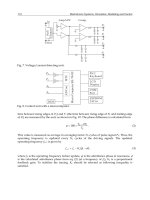
Basd on Eqs.(34)-(36), input impedance as a function of frequency at different load
resistances are calculated and shown in Fig.7. And the experimental results are shown in
Fig.8. In the input impedance of the PT with load resistance varied from short (R
L
=0) to
open (R
L
=∞), it shows that the peak frequency is changed from 94.05 kHz to 97.85 kHz. The
peak frequency is increased as the load resistance is increased. Also, there exists an optimal
load resistance R
L,opt
, which shows the maximum damping ratio in the input impedance
when compared with the other different load resistances. We can also calculated the
optimal load resistance R
L,opt
=2.6 kΩ from Eq.(52). It should be noted that efficiency of the
PT approaches to the maximum efficiency when the load resistance R
L
approaches the
optimal load resistance R
L,opt
.
Fig. 4. Mode shapes of the piezoelectric transformer.
(a) 1st vibration mode (b) 2nd vibration mode (c) 3rd vibration mode
Fig. 5. Vibration modes of piezoelectric transformer.
Fig. 6. Input and output impedance
4.2 Voltage Step-up Ratio, Output Power, and Efficiency
The experimental setup for the measurement of the voltage step-up ratio and output power
of the PT is illustrated in Fig.9. A function generator (NF Corporation, WF1943) and a high
frequency amplifier (NF Corporation, HSA4011) were used for driving power supply. The
variation in electric characteristics with load resistance and driving frequency were
measured with a multi-meter (Agilent 34401A). The voltage step-up ratios as a function of
frequency at different load resistances were measured and compared with theoretical
analysis, as shown in Fig.10. It shows that the experimental results are in a good agreement
with the theoretical results, so the proposed electromechanical model for the PT was
verified.
Fig. 7. Experimental setup
MechatronicSystems,Simulation,ModellingandControl14
Piezoelectric coefficient d
31
-125×10
-12
C/N
Coupling factor k
p
0.59
Mechanical quality factor Q
m
500
Dielectric constant ε
33
/ε
0
1694
Density ρ 7600 g/cm
3
Young’s modulus Y
11
E
8×10
10
N/m
2
Table 1. Properties of piezoelectric material.
Input piezoelectric capacitance C
i
1.5nF
Output piezoelectric capacitance C
o
671.5pF
Input turn ratio A
i
0.1198
Output turn ratio A
o
0.07545
Effective mass m
1
4.773×10
-4
kg
Effective damping d
1
1.868 N-s/m
Effective stiffness k
1
1.569×10
8
N/m
Table 2. Parameters of the equivalent circuit
Fig. 8. Calculated input impedance
Fig. 9. Measured input impedance
Fig. 10. Voltage step-up ratio
ElectromechanicalAnalysisofaRing-typePiezoelectricTransformer 15
Piezoelectric coefficient d
31
-125×10
-12
C/N
Coupling factor k
p
0.59
Mechanical quality factor Q
m
500
Dielectric constant ε
33
/ε
0
1694
Density ρ 7600 g/cm
3
Young’s modulus Y
11
E
8×10
10
N/m
2
Table 1. Properties of piezoelectric material.
Input piezoelectric capacitance C
i
1.5nF
Output piezoelectric capacitance C
o
671.5pF
Input turn ratio A
i
0.1198
Output turn ratio A
o
0.07545
Effective mass m
1
4.773×10
-4
kg
Effective damping d
1
1.868 N-s/m
Effective stiffness k
1
1.569×10
8
N/m
Table 2. Parameters of the equivalent circuit
Fig. 8. Calculated input impedance
Fig. 9. Measured input impedance
Fig. 10. Voltage step-up ratio
MechatronicSystems,Simulation,ModellingandControl16
5. Conclusion
In this chapter, an electromechanical model for ring-type PT is presented. An equivalent
circuit of the PT is shown based on the electromechanical model. Also, the voltage step-up
ratio, input impedance, output impedance, and output power of the PT are calculated, and
the optimal load resistance and the maximum efficiency for the PT have been obtained. In
the last, some simulated results of the electromechanical model are compared with the
experimental results for verification. The model presented here lays foundation for a
general framework capable of serving a useful design tool for optimizing the configuration
of the PT.
6. References
Bishop, R. P. (1998). Multi-Layer Piezoelectric Transformer, US Patent No.5834882.
Hagood, N. W. Chung, W. H. Flotow, A. V. (1990). Modeling of Piezoelectric Acatuator
Dynamics for Active Structural Control. Intell. Mater. Syst. And Struct., Vol.1, pp.
327-354, ISSN:1530-8138.
Hu, J. H. Li, H. L. Chan, H. L. W. Choy, C. L. (2001). A Ring-shaped Piezoelectric
Transformer Operating in the third Sysmmetric Extenxional Vibration Mode.
Sensors and Actuators, A., No.88, pp. 79-86, ISSN:0924-4247.
Laoratanakul, P. Carazo, A. V. Bouchilloux P. Uchino, K. (2002). Unipoled Disk-type
Piezoelectric Transformers. Jpn. J. Appl. Phys., Vol.41, No., pp. 1446-1450,
ISSN:1347-4065.
Rosen, C. A. (1956). Ceramic Transformers and Filters, Proceedings of Electronic Comp., pp.
205-211.
Sasaki, Y. Uehara, K. Inoue, T. (1993). Piezoelectric Ceramic Transformer Being Driven with
Thickness Extensional Vibration, US Patent No.5241236.
GeneticAlgorithm–BasedOptimalPWMinHighPower
SynchronousMachinesandRegulationofObservedModulationError 17
Genetic Algorithm–Based Optimal PWM in High Power Synchronous
MachinesandRegulationofObservedModulationError
AlirezaRezazade,ArashSayyahandMitraAaki
x
Genetic Algorithm–Based Optimal PWM in
High Power Synchronous Machines and
Regulation of Observed Modulation Error
Alireza Rezazade
Shahid Beheshti University G.C.
Arash Sayyah
University of Illinois at Urbana-Champaign
Mitra Aflaki
SAIPA Automotive Industries Research and Development Center
1. Introduction
UNIQUE features of synchronous machines like constant-speed operation, producing
substantial savings by supplying reactive power to counteract lagging power factor caused
by inductive loads, low inrush currents, and capabilities of designing the torque
characteristics to meet the requirements of the driven load, have made them the optimal
choices for a multitude of industries. Economical utilization of these machines and also
increasing their efficiencies are issues that should receive significant attention. At high
power rating operation, where high switching efficiency in the drive circuits is of utmost
importance, optimal PWM is the logical feeding scheme. That is, an optimal value for each
switching instant in the PWM waveforms is determined so that the desired fundamental
output is generated and the predefined objective function is optimized (Holtz , 1992).
Application of optimal PWM decreases overheating in machine and results in diminution of
torque pulsation. Overheating resulted from internal losses, is a major factor in rating of
machine. Moreover, setting up an appropriate cooling method is a particularly serious issue,
increasing in intricacy with machine size. Also, from the view point of torque pulsation,
which is mainly affected by the presence of low-order harmonics, will tend to cause jitter in
the machine speed. The speed jitter may be aggravated if the pulsing torque frequency is
low, or if the system mechanical inertia is small. The pulsing torque frequency may be near
the mechanical resonance of the drive system, and these results in severe shaft vibration,
causing fatigue, wearing of gear teeth and unsatisfactory performance in the feedback
control system.
Amongst various approaches for achieving optimal PWM, harmonic elimination method is
predominant (Mohan et al., 2003), (Chiasson et al., 2004), (Sayyah et al., 2006), (Sun et al.,
1996), (Enjeti et al., 1990). One of the disadvantages associated with this method originates
from this fact that as the total energy of the PWM waveform is constant, elimination of low-
order harmonics substantially boosts remaining ones. Since copper losses are fundamentally
2
MechatronicSystems,Simulation,ModellingandControl18
determined by current harmonics, defining a performance index related to undesirable
effects of the harmonics is of the essence in lieu of focusing on specific harmonics (Bose BK,
2002). Herein, the total harmonic current distortion (THCD) is the objective function for
minimization of machine losses. The fundamental frequency is necessarily considered
constant in this case, in order to define a sensible optimization problem (i.e. “Pulse width
modulation for Holtz, J. 1996”).
In this chapter, we have strove to propose an appropriate current harmonic model for high
power synchronous motors by thorough inspecting the main structure of the machine (i.e.
“The representation of Holtz, J 1995”), (Rezazade et al.,2006), (Fitzgerald et al., 1983),
(Boldea & Nasar, 1992). Possessing asymmetrical structure in direct axis (d- axis) and
quadrature axis (q-axis) makes a great difference in modelling of these motors relative to
induction ones. The proposed model includes some internal parameters which are not part
of machines characteristics. On the other hand, machines d and q axes inductances are
designed so as to operate near saturation knee of magnetization curve. A slight change in
operating point may result in large changes in these inductances. In addition, some factors
like aging and temperature rise can influence the harmonic model parameters.
Based on gathered input and output data at a specific operating point, these internal
parameters are determined using online identification methods (Åström & Wittenmark,
1994), (Ljung & Söderström, 1983). In light of the identified parameters, the problem has
been redrafted as an optimization task, and optimal pulse patterns are sought through
genetic algorithm (GA) (Goldberg, 1989), (Michalewicz, 1989), (Fogel, 1995), (Davis, 1991),
(Bäck, 1996), (Deb, 2001), (Liu, 2002). Indeed, the complexity and nonlinearity of the
proposed objective function increases the probability of trapping the conventional
optimization methods in suboptimal solutions. The GA provided with salient features can
effectively cope with shortcomings of the deterministic optimization methods, particularly
when decision variables increase. The advantages of this optimization are so remarkable
considering the total power of the system. Optimal PWM waveforms are accomplished up
to 12 switches (per quarter period of PWM waveform), in which for more than this number
of switching angles, space vector PWM (SVPWM) method, is preferred to optimal PWM
approach. During real-time operation, the required fundamental amplitude is used for
addressing the corresponding switching angles, which are stored in a read-only memory
(ROM) and served as a look-up table for controlling the inverter.
Optimal PWM waveforms are determined for steady state conditions. Presence of step
changes in trajectories of optimal pulse patterns results in severe over currents which in turn
have detrimental effects on a high-performance drive system. Without losing the feed
forward structure of PWM fed inverters, considerable efforts should have gone to mitigate
the undesired transient conditions in load currents. The inherent complexity of
synchronous machines transient behaviour can be appreciated by an accurate representation
of significant circuits when transient conditions occur. Several studies have been done for
fast current tracking control in induction motors (Holtz & Beyer, 1991), (Holtz & Beyer,
1994), (Holtz & Beyer, 1993), (Holtz & Beyer, 1995). In these studies, the total leakage
inductance is used as current harmonic model for induction motors. As mentioned earlier,
due to asymmetrical structure in d and q axes conditions in synchronous motors, derivation
of an appropriate current harmonic model for dealing with transient conditions seems
indispensable which is covered in this chapter. The effectiveness of the proposed method for
fast tracking control has been corroborated by establishing an experimental setup, where a
field excited synchronous motor in the range of 80 kW drives an induction generator as the
load. Rapid disappearance of transients is observed.
2. Optimal Synchronous PWM for Synchronous Motors
2.1 Machine Model
Electrical machines with rotating magnetic field are modelled based upon their applications
and feeding scheme. Application of these machines in variable speed electrical drives has
significantly increased where feed forward PWM generation has proven its effectiveness as
a proper feeding scheme. Furthermore, some simplifications and assumptions are
considered in modelling of these machines, namely space harmonics of the flux linkage
distribution are neglected, linear magnetic due to operation in linear portion of
magnetization curve prior to experiencing saturation knee is assumed, iron losses are
neglected, slot harmonics and deep bar effects are not considered. In light of mentioned
assumptions, the resultant model should have the capability of addressing all circumstances
in different operating conditions (i.e. steady state and transient) including mutual effects of
electrical drive system components, and be valid for instant changes in voltage and current
waveforms. Such a model is attainable by Space Vector theory (i.e. “On the spatial
propagation of Holtz, J 1996”).
Synchronous machine model equations can be written as follows:
,
R
R S R
S
S S R S
d
j
d
Ψ
u r i Ψ
(1)
0 ,
D
D D
d
d
Ψ
R i
(2)
,
R S R
S S R m
Ψ l i Ψ
(3)
,
R
m m D F
Ψ l i i
(4)
,
D D D m S F
Ψ l i l i i
(5)
where:
0
1
, ,
0
0
d
S lS m F F
q
l
i
l
l l l i
(6)
0 0
,
0 0
md Dd
m D
mq Dq
l l
l l
l l
(7)
where
d
l
and
q
l
are inductances of the motor in d and q axes;
D
i
is damper winding current;
R
S
u
and
R
S
i
are stator voltage and current space vectors, respectively;
D
l is the damper
GeneticAlgorithm–BasedOptimalPWMinHighPower
SynchronousMachinesandRegulationofObservedModulationError 19
determined by current harmonics, defining a performance index related to undesirable
effects of the harmonics is of the essence in lieu of focusing on specific harmonics (Bose BK,
2002). Herein, the total harmonic current distortion (THCD) is the objective function for
minimization of machine losses. The fundamental frequency is necessarily considered
constant in this case, in order to define a sensible optimization problem (i.e. “Pulse width
modulation for Holtz, J. 1996”).
In this chapter, we have strove to propose an appropriate current harmonic model for high
power synchronous motors by thorough inspecting the main structure of the machine (i.e.
“The representation of Holtz, J 1995”), (Rezazade et al.,2006), (Fitzgerald et al., 1983),
(Boldea & Nasar, 1992). Possessing asymmetrical structure in direct axis (d- axis) and
quadrature axis (q-axis) makes a great difference in modelling of these motors relative to
induction ones. The proposed model includes some internal parameters which are not part
of machines characteristics. On the other hand, machines d and q axes inductances are
designed so as to operate near saturation knee of magnetization curve. A slight change in
operating point may result in large changes in these inductances. In addition, some factors
like aging and temperature rise can influence the harmonic model parameters.
Based on gathered input and output data at a specific operating point, these internal
parameters are determined using online identification methods (Åström & Wittenmark,
1994), (Ljung & Söderström, 1983). In light of the identified parameters, the problem has
been redrafted as an optimization task, and optimal pulse patterns are sought through
genetic algorithm (GA) (Goldberg, 1989), (Michalewicz, 1989), (Fogel, 1995), (Davis, 1991),
(Bäck, 1996), (Deb, 2001), (Liu, 2002). Indeed, the complexity and nonlinearity of the
proposed objective function increases the probability of trapping the conventional
optimization methods in suboptimal solutions. The GA provided with salient features can
effectively cope with shortcomings of the deterministic optimization methods, particularly
when decision variables increase. The advantages of this optimization are so remarkable
considering the total power of the system. Optimal PWM waveforms are accomplished up
to 12 switches (per quarter period of PWM waveform), in which for more than this number
of switching angles, space vector PWM (SVPWM) method, is preferred to optimal PWM
approach. During real-time operation, the required fundamental amplitude is used for
addressing the corresponding switching angles, which are stored in a read-only memory
(ROM) and served as a look-up table for controlling the inverter.
Optimal PWM waveforms are determined for steady state conditions. Presence of step
changes in trajectories of optimal pulse patterns results in severe over currents which in turn
have detrimental effects on a high-performance drive system. Without losing the feed
forward structure of PWM fed inverters, considerable efforts should have gone to mitigate
the undesired transient conditions in load currents. The inherent complexity of
synchronous machines transient behaviour can be appreciated by an accurate representation
of significant circuits when transient conditions occur. Several studies have been done for
fast current tracking control in induction motors (Holtz & Beyer, 1991), (Holtz & Beyer,
1994), (Holtz & Beyer, 1993), (Holtz & Beyer, 1995). In these studies, the total leakage
inductance is used as current harmonic model for induction motors. As mentioned earlier,
due to asymmetrical structure in d and q axes conditions in synchronous motors, derivation
of an appropriate current harmonic model for dealing with transient conditions seems
indispensable which is covered in this chapter. The effectiveness of the proposed method for
fast tracking control has been corroborated by establishing an experimental setup, where a
field excited synchronous motor in the range of 80 kW drives an induction generator as the
load. Rapid disappearance of transients is observed.
2. Optimal Synchronous PWM for Synchronous Motors
2.1 Machine Model
Electrical machines with rotating magnetic field are modelled based upon their applications
and feeding scheme. Application of these machines in variable speed electrical drives has
significantly increased where feed forward PWM generation has proven its effectiveness as
a proper feeding scheme. Furthermore, some simplifications and assumptions are
considered in modelling of these machines, namely space harmonics of the flux linkage
distribution are neglected, linear magnetic due to operation in linear portion of
magnetization curve prior to experiencing saturation knee is assumed, iron losses are
neglected, slot harmonics and deep bar effects are not considered. In light of mentioned
assumptions, the resultant model should have the capability of addressing all circumstances
in different operating conditions (i.e. steady state and transient) including mutual effects of
electrical drive system components, and be valid for instant changes in voltage and current
waveforms. Such a model is attainable by Space Vector theory (i.e. “On the spatial
propagation of Holtz, J 1996”).
Synchronous machine model equations can be written as follows:
,
R
R S R
S
S S R S
d
j
d
Ψ
u r i Ψ
(1)
0 ,
D
D D
d
d
Ψ
R i
(2)
,
R S R
S S R m
Ψ l i Ψ
(3)
,
R
m m D F
Ψ l i i
(4)
,
D D D m S F
Ψ l i l i i
(5)
where:
0
1
, ,
0
0
d
S lS m F F
q
l
i
l
l l l i
(6)
0 0
,
0 0
md Dd
m D
mq Dq
l l
l l
l l
(7)
where
d
l
and
q
l
are inductances of the motor in d and q axes;
D
i
is damper winding current;
R
S
u
and
R
S
i
are stator voltage and current space vectors, respectively;
D
l is the damper
GeneticAlgorithm–BasedOptimalPWMinHighPower
SynchronousMachinesandRegulationofObservedModulationError 21
inductance;
md
l
is the d-axis magnetization inductance;
mq
l
is the q-axis magnetization
inductance;
Dq
l
is the d-axis damper inductance;
Dd
l
is the q-axis damper inductance;
m
Ψ
is the magnetization flux;
D
Ψ
is the damper flux;
F
i
is the field excitation current. Time is
also normalized as
t
, where
is the angular frequency. The block diagram model of
the machine is illustrated in Figure 1. With the presence of excitation current and its control
loop, it is assumed that a current source is used for synchronous machine excitation; thereby
excitation current dynamic is neglected. As can be observed in Figure 1, harmonic
component of
D
i
or
F
i
is not negligible; accordingly harmonic component of
m
Ψ
should
be taken into account and simplifications which are considered in induction machines for
current harmonic component are not applicable herein. Therefore, utilization of
synchronous machine complete model for direct observation of harmonic component of
stator current
h
i
is indispensable. This issue is subjected to this chapter.
Fig. 1. Schematic block diagram of electromechanical system of synchronous machine.
2.2 Waveform Representation
For the scope of this chapter, a PWM waveform is a
2
periodic function
f
with two
distinct normalized levels of -1, +1 for
0 2
and has the symmetries
ff
and
2ff
. A normalized PWM waveform is shown in
Figure 2.
Fig. 2. One Line-to-Neutral PWM structure.
Owing to the symmetries in PWM waveform of Figure 2, only the odd harmonics exist. As
such,
f
can be written with the Fourier series as
, 5,3,1
sin
k
k
kuf
(8)
with
2
0
1
1
4
sin
4
1 2 1 cos .
k
N
i
i
i
u f k
k
k
(9)
2.3 THCD Formulation
The total harmonic current distortion is defined as follows:
2
1
1
,
i S S
T
t t dt
T
i i
(10)
where
1S
i
is the fundamental component of stator current.
Assuming that the steady state operation of machine makes a constant exciting current, the
dampers current in the system can be neglected. Therefore, the equation of the machine
model in rotor coordinates can be written as:
R
R R R
S
S S S S S m F S
d
j j
d
i
u r i l i l i l
(11)
With the Park transformation, the equation of the machine model in stator coordinates (the
so called α-β coordinates) can be written as:
sin 2 cos 2
cos 2 sin 2
2
cos 2 sin 2 sin
,
sin 2 cos 2 cos
2
d q
S d q
d q
md F
l l
d
R l l
d
l l
d
l i
d
i
u i i
i
(12)
where
is the rotor angle. Neglecting the ohmic terms in (12), we have:
MechatronicSystems,Simulation,ModellingandControl22
cos
,
sin
S md F
d d
l i
d d
u l i
(13)
where:
2
cos 2 sin 2
.
sin 2 cos 2
2 2
d q d q
S
l l l l
l I
(14)
I
2
is the 2×2 identity matrix. Hence:
1
2
cos
.
sin
cos 2 sin 2
2 2 2
cos
.
sin
sin 2 cos 2
2 2 2
co
2 2
S md F
d q d q d q
d q d q d q
md F
d q d q d q
d q d q d q
d q d q
d q d q
d l i
l l l l l l
l l l l l l
d l i
l l l l l l
l l l l l l
l l l l
I
l l l l
i l u
u
s 2 sin 2 cos
.
sin 2 cos 2 sin
md F
d l i
u
(15)
With further simplification, we have
i
can be written as:
1
2
cos cos 2 sin 2 cos
.
sin sin 2 cos 2 sin
2 2 2
cos 2 sin 2
.
sin 2 cos 2
2
d q d q d q
md F md
d q d q d q
J
d q
d q
J
l l l l l l
d l i l
l l l l l l
l l
d
l l
i u
u
(16)
Using the trigonometric identities,
1 2 1 2 1 2
cos cos cos sin sin
and
1 2 1 2 1 2
sin sin cos cos sin
the term
1
J
in Equation (16) can be
simplified as:
1
cos cos 2 .cos sin 2 .sin
sin sin 2 .cos cos 2 .cos
2 2
cos cos
sin sin
2 2
cos
.
sin
d q d q
md F md F
d q d q
d q d q
md F md F
d q d q
md
F
d
l l l l
J l i l i
l l l l
l l l l
l i l i
l l l l
l
i
l
(17)
On the other hand, writing the phase voltages in Fourier series:
3
12sin
12
Ss
sA
suu
,
3
3
2
12sin
12
Ss
sB
suu
and
3
3
4
12sin
12
Ss
sC
suu
; then using 3-phase to 2-phase
transformation, we have:
3
3
3
2
sin
sin
3
1
Ss
ss
Ss
s
CB
A
su
su
uu
u
u
u
(18)
in which:
1,7,13,
6
5,11,17,
6
s
for s
for s
(19)
As such, we have:
6 1 6 5
0
6 1 6 5
0
sin 6 1 sin 6 5
.
2 2
sin 6 1 sin 6 5
3 6 3 6
l l
l
l l
l
u l u l
u l u l
u
(20)
Integration of
u
yields:
GeneticAlgorithm–BasedOptimalPWMinHighPower
SynchronousMachinesandRegulationofObservedModulationError 23
cos
,
sin
S md F
d d
l i
d d
u l i
(13)
where:
2
cos 2 sin 2
.
sin 2 cos 2
2 2
d q d q
S
l l l l
l I
(14)
I
2
is the 2×2 identity matrix. Hence:
1
2
cos
.
sin
cos 2 sin 2
2 2 2
cos
.
sin
sin 2 cos 2
2 2 2
co
2 2
S md F
d q d q d q
d q d q d q
md F
d q d q d q
d q d q d q
d q d q
d q d q
d l i
l l l l l l
l l l l l l
d l i
l l l l l l
l l l l l l
l l l l
I
l l l l
i l u
u
s 2 sin 2 cos
.
sin 2 cos 2 sin
md F
d l i
u
(15)
With further simplification, we have
i
can be written as:
1
2
cos cos 2 sin 2 cos
.
sin sin 2 cos 2 sin
2 2 2
cos 2 sin 2
.
sin 2 cos 2
2
d q d q d q
md F md
d q d q d q
J
d q
d q
J
l l l l l l
d l i l
l l l l l l
l l
d
l l
i u
u
(16)
Using the trigonometric identities,
1 2 1 2 1 2
cos cos cos sin sin
and
1 2 1 2 1 2
sin sin cos cos sin
the term
1
J
in Equation (16) can be
simplified as:
1
cos cos 2 .cos sin 2 .sin
sin sin 2 .cos cos 2 .cos
2 2
cos cos
sin sin
2 2
cos
.
sin
d q d q
md F md F
d q d q
d q d q
md F md F
d q d q
md
F
d
l l l l
J l i l i
l l l l
l l l l
l i l i
l l l l
l
i
l
(17)
On the other hand, writing the phase voltages in Fourier series:
3
12sin
12
Ss
sA
suu
,
3
3
2
12sin
12
Ss
sB
suu
and
3
3
4
12sin
12
Ss
sC
suu
; then using 3-phase to 2-phase
transformation, we have:
3
3
3
2
sin
sin
3
1
Ss
ss
Ss
s
CB
A
su
su
uu
u
u
u
(18)
in which:
1,7,13,
6
5,11,17,
6
s
for s
for s
(19)
As such, we have:
6 1 6 5
0
6 1 6 5
0
sin 6 1 sin 6 5
.
2 2
sin 6 1 sin 6 5
3 6 3 6
l l
l
l l
l
u l u l
u l u l
u
(20)
Integration of
u
yields:
MechatronicSystems,Simulation,ModellingandControl24
6 1 6 5
0
6 1 6 5
0
6 1 6 5
0
6 1
cos 6 1 cos 6 5
6 1 6 5
1
.
3
cos 6 1 4 cos 6 5 4
6 1 2 6 5 2
cos 6 1 cos 6 5
6 1 6 5
1
6
l l
l
l l
l
l l
l
l
u u
l l
l l
d
u u
l l l l
l l
u u
l l
l l
u
l
u
6 5
0
.
sin 6 1 sin 6 5
1 6 5
l
l
u
l l
l
(21)
By substitution of
du in Equation (16), the term J
2
can be written as:
2
6 1
0
6 1
0
6 5
cos 2 sin 2
.
sin 2 cos 2
cos 6 1 .cos 2 sin 6 1 .sin 2
6 1
1
. .
cos 6 1 .sin 2 sin 6 1 .cos 2
6 1
cos 6 5 .cos 2 sin 6 5
6 5
l
l
l
l
l
J d
u
l l
l
u
l l
l
u
l l
l
u
0
6 5
0
6 1 6 5
0
6 1 6 5
0
.sin 2
cos 6 5 .sin 2 sin 6 5 .cos 2
6 5
cos 6 1 cos 6 7
6 1 6 5
1
sin 6 1 sin 6 7
6 1 6 5
l
l
l
l l
l
l l
l
u
l l
l
u u
l l
l l
u u
l l
l l
.
(22)
Considering the derived results, we can rewrite
ii
A
as:
6 1 6 5
0
6 1 6 5
0
cos 6 1 cos 6 5
2 6 1 6 5
cos 6 1 cos 6 7
2 6 1 6 5
cos .
d q
l l
A
l
d q
d q
l l
l
d q
md
F
d
l l
u u
i l l
l l l l
l l
u u
l l
l l l l
l
i
l
(23)
Using the appropriate dummy variables 1
ll and 1
ll , we have:
6 1 6 5
1 1
6 7 6 1
0 0
6 1 6
0
cos 6 5 cos 6 5
2 6 1 6 5
cos 6 1 cos 6 1 cos
2 6 7 6 1
cos 6 1
2 6 1
d q
l l
A
d q
l l
d q
l l md
F
d q d
l l
d q
l
d q
l
l l
u u
i l l
l l l l
l l
u u l
l l i
l l l l l
l l
u u
l
l l l
5
0
6 7 6 1
1
0 0
cos 6 5
6 5
cos 6 5 cos 6 1 cos cos
2 6 7 6 1
l
l
d q
l l md
F
d q d
l l
l
l
l l
u u l
l l u i
l l l l l
(24)
Thus, we have
A
i
as:
6 1 6 1
0
6 5 6 7
1
0
1
.cos 6 1
2 6 1 6 1
cos .cos 6 1
6 5 6 7
cos .
l l
A d q d q
l
d q
l l
d q d q d q
l
md
F
d
u u
i l l l l l
l l l l
u u
l l u l l l l l
l l
l
i
l
(25)
Removing the fundamental components from Equation (25), the current harmonic is
introduced as:
6 1 6 1
1
6 5 6 7
0
6 7 6 5
0
1
. .cos 6 1
2 6 1 6 1
.cos 6 5
6 5 6 7
1
. .cos 6 7
2 6 7 6 5
l l
Ah d q d q
l
d q
l l
d q d q
l
l l
d q d q
l
d q
u u
i l l l l l
l l l l
u u
l l l l l
l l
u u
l l l l l
l l l l
l
6 5 6 7
0
.cos 6 5 .
6 5 6 7
l l
d q d q
l
u u
l l l l
l l
(26)
On the other hand,
2
l
can be written as:
GeneticAlgorithm–BasedOptimalPWMinHighPower
SynchronousMachinesandRegulationofObservedModulationError 25
6 1 6 5
0
6 1 6 5
0
6 1 6 5
0
6 1
cos 6 1 cos 6 5
6 1 6 5
1
.
3
cos 6 1 4 cos 6 5 4
6 1 2 6 5 2
cos 6 1 cos 6 5
6 1 6 5
1
6
l l
l
l l
l
l l
l
l
u u
l l
l l
d
u u
l l l l
l l
u u
l l
l l
u
l
u
6 5
0
.
sin 6 1 sin 6 5
1 6 5
l
l
u
l l
l
(21)
By substitution of
du in Equation (16), the term J
2
can be written as:
2
6 1
0
6 1
0
6 5
cos 2 sin 2
.
sin 2 cos 2
cos 6 1 .cos 2 sin 6 1 .sin 2
6 1
1
. .
cos 6 1 .sin 2 sin 6 1 .cos 2
6 1
cos 6 5 .cos 2 sin 6 5
6 5
l
l
l
l
l
J d
u
l l
l
u
l l
l
u
l l
l
u
0
6 5
0
6 1 6 5
0
6 1 6 5
0
.sin 2
cos 6 5 .sin 2 sin 6 5 .cos 2
6 5
cos 6 1 cos 6 7
6 1 6 5
1
sin 6 1 sin 6 7
6 1 6 5
l
l
l
l l
l
l l
l
u
l l
l
u u
l l
l l
u u
l l
l l
.
(22)
Considering the derived results, we can rewrite
ii
A
as:
6 1 6 5
0
6 1 6 5
0
cos 6 1 cos 6 5
2 6 1 6 5
cos 6 1 cos 6 7
2 6 1 6 5
cos .
d q
l l
A
l
d q
d q
l l
l
d q
md
F
d
l l
u u
i l l
l l l l
l l
u u
l l
l l l l
l
i
l
(23)
Using the appropriate dummy variables 1
ll and 1
ll , we have:
6 1 6 5
1 1
6 7 6 1
0 0
6 1 6
0
cos 6 5 cos 6 5
2 6 1 6 5
cos 6 1 cos 6 1 cos
2 6 7 6 1
cos 6 1
2 6 1
d q
l l
A
d q
l l
d q
l l md
F
d q d
l l
d q
l
d q
l
l l
u u
i l l
l l l l
l l
u u l
l l i
l l l l l
l l
u u
l
l l l
5
0
6 7 6 1
1
0 0
cos 6 5
6 5
cos 6 5 cos 6 1 cos cos
2 6 7 6 1
l
l
d q
l l md
F
d q d
l l
l
l
l l
u u l
l l u i
l l l l l
(24)
Thus, we have
A
i
as:
6 1 6 1
0
6 5 6 7
1
0
1
.cos 6 1
2 6 1 6 1
cos .cos 6 1
6 5 6 7
cos .
l l
A d q d q
l
d q
l l
d q d q d q
l
md
F
d
u u
i l l l l l
l l l l
u u
l l u l l l l l
l l
l
i
l
(25)
Removing the fundamental components from Equation (25), the current harmonic is
introduced as:
6 1 6 1
1
6 5 6 7
0
6 7 6 5
0
1
. .cos 6 1
2 6 1 6 1
.cos 6 5
6 5 6 7
1
. .cos 6 7
2 6 7 6 5
l l
Ah d q d q
l
d q
l l
d q d q
l
l l
d q d q
l
d q
u u
i l l l l l
l l l l
u u
l l l l l
l l
u u
l l l l l
l l l l
l
6 5 6 7
0
.cos 6 5 .
6 5 6 7
l l
d q d q
l
u u
l l l l
l l
(26)
On the other hand,
2
l
can be written as:
MechatronicSystems,Simulation,ModellingandControl26
2 2
2
6 7 6 5 6 5 6 7
2 2
2 2 2 2 2 2
6 7 6 5 6 5 6 7
6 7 6 5 6 5 6 7
2 2 4 .
6 7 6 5 6 5 6 7
l l l l
l d q d q d q d q
q
l l l l
d q d q d q
u u u u
l l l l l l l l
l l l l
u u u u
l l l l l l
l l l l
(27)
With normalization of
2
l
; i.e.
2
2
2 2
l
l
d q
l l
and also the definition of the total harmonic
current distortion as
2
2
0
l
i
l
, it can be simplified as:
2 2
2 2
2
6 5 6 7 6 5 6 7
2 2
0
2 .
6 5 6 7 6 5 6 7
d q
l l l l
i
l
d q
l l
u u u u
l l l l l l
(28)
Considering the set
, 13,11,7,5
3
S
and with more simplification,
i
in high-power
synchronous machines can be explicitly expressed as:
3
2
2 2
6 1 6 1
2 2
1
2 . .
6 1 6 1
d q
k l l
i
k S l
d q
l l
u u u
k l l l l
(29)
As mentioned earlier, THCD in high-power synchronous machines depends on
d
l
and
q
l
,
the inductances of d and q axes, respectively. Needless to say, switching angles:
N
, ,,
21
determine the voltage harmonics in Equation (29). Hence, the optimization
problem consists of identification of the
dq
ll
for the under test synchronous machine;
determination of these switching angles as decision variables so that the
i
is minimized. In
addition, throughout the optimization procedure, it is desired to maintain the fundamental
output voltage at a constant level:
1
u M
. M, the so-called the modulation index may be
assumed to have any value between 0 and
4
. It can be shown that
N
is dependent on
modulation index and the rest of N-1 switching angles. As such, one decision variable can be
eliminated explicitly. More clearly:
Minimize
3
2
2
2
6 1 6 1
2
1
1
2 .
6 1 6 1
1
q d
k l l
i
k S l
q d
l l
u u u
k l l
l l
(30)
Subject to
2
0
121
N
and
1
4
cos12
2
1
cos
1
1
1
1
1
M
N
i
i
i
N
N
(31)
3. Switching Scheme
Switching frequency in high-power systems, due to the use of GTOs in the inverter is
limited to several hundred hertz. In this chapter, the switching frequency has been set to
200
s
f
Hz
. Considering the frequency of the fundamental component of PWM
waveform to be variable with maximum value of 50 Hz (i.e.
1max
50
f
Hz
), then
1max
4
s
f f
. This condition forces a constraint on the number of switches, since:
N
f
f
s
1
(32)
On the other hand, in the machines with rotating magnetic field, in order to maintain the
torque at a constant level, the fundamental frequency of the PWM should be proportional
to its amplitude (modulation index is also proportional to the amplitude) (Leonhard, 2001).
That is:
max1
max1
1
f
f
N
f
kf
N
k
kfM
s
s
(33)
Also, we have:
.
1
1|
max1
1
max11
f
kkfM
ff
(34)
Considering Equations (33) and (34), the following equation is resulted:
max1
NM
f
f
s
(35)
The value of
1maxs
f
f
is plotted versus modulation index in Figure 3.
Figure 3 shows that as the number of switching angles increases and M declines from unity,
the curve moves towards the upper limit
1maxs
f
f
. The curve, however, always remains
under the upper limit. When N increases and reaches a large amount, optimization
procedure and its accomplished results are not effective. Additionally, it does not show a
significant advantage in comparison with SVPWM (space vector PWM). Based on this fact,
in high power machines, the feeding scheme is a combination of optimized PWM and
SVPWM.
At this juncture, feed-forward structure of PWM fed inverter is emphasized. Presence of
current feedback path means that the switching frequency is dictated by the current which is
the follow-on of system dynamics and load conditions. This may give rise to uncontrollable
high switching frequencies that indubitably denote colossal losses. Furthermore, utilization
of current feedback for PWM generation intensifies system instability and results in chaos.
GeneticAlgorithm–BasedOptimalPWMinHighPower
SynchronousMachinesandRegulationofObservedModulationError 27
2 2
2
6 7 6 5 6 5 6 7
2 2
2 2 2 2 2 2
6 7 6 5 6 5 6 7
6 7 6 5 6 5 6 7
2 2 4 .
6 7 6 5 6 5 6 7
l l l l
l d q d q d q d q
q
l l l l
d q d q d q
u u u u
l l l l l l l l
l l l l
u u u u
l l l l l l
l l l l
(27)
With normalization of
2
l
; i.e.
2
2
2 2
l
l
d q
l l
and also the definition of the total harmonic
current distortion as
2
2
0
l
i
l
, it can be simplified as:
2 2
2 2
2
6 5 6 7 6 5 6 7
2 2
0
2 .
6 5 6 7 6 5 6 7
d q
l l l l
i
l
d q
l l
u u u u
l l l l l l
(28)
Considering the set
, 13,11,7,5
3
S
and with more simplification,
i
in high-power
synchronous machines can be explicitly expressed as:
3
2
2 2
6 1 6 1
2 2
1
2 . .
6 1 6 1
d q
k l l
i
k S l
d q
l l
u u u
k l l l l
(29)
As mentioned earlier, THCD in high-power synchronous machines depends on
d
l
and
q
l
,
the inductances of d and q axes, respectively. Needless to say, switching angles:
N
, ,,
21
determine the voltage harmonics in Equation (29). Hence, the optimization
problem consists of identification of the
dq
ll
for the under test synchronous machine;
determination of these switching angles as decision variables so that the
i
is minimized. In
addition, throughout the optimization procedure, it is desired to maintain the fundamental
output voltage at a constant level:
1
u M
. M, the so-called the modulation index may be
assumed to have any value between 0 and
4
. It can be shown that
N
is dependent on
modulation index and the rest of N-1 switching angles. As such, one decision variable can be
eliminated explicitly. More clearly:
Minimize
3
2
2
2
6 1 6 1
2
1
1
2 .
6 1 6 1
1
q d
k l l
i
k S l
q d
l l
u u u
k l l
l l
(30)
Subject to
2
0
121
N
and
MechatronicSystems,Simulation,ModellingandControl108
The transducer was vertically contacted with a transparent object (an acrylic resin) with a
contact load. The vibrometer laser beam was irradiated through the resin, as shown in Fig. 3.
Through the measurement, operating frequency was swept with constant amplitude of
driving voltage. Frequency responses of the vibration amplitude with the change of contact
load are shown in Fig. 4. Admittance phases are also shown in the figure. Local peaks of the
amplitude mean resonance frequencies. It can be seen that resonance frequency shifts to the
higher frequency region according to the increase of the contact load. Admittance phase
changes dramatically around the resonance and meets a certain value (around 0 [deg]: same
as the previous result) at the resonance frequency.
3. Resonance Frequency Tracing System
3.1 Overview
As described in the previous section, resonance frequency of the Langevin type ultrasonic
transducer changes according to the various reasons. To keep strong vibration, resonance
frequency should be traced during the operation of the transducer. In this research, tracing
system based on admittance phase measurement is proposed. A microcomputer was
applied for the measurement. Tracing algorithm was also embedded in the computer. Other
intelligent functions such as communication with other devices can be installed to the
computer. Therefore, this system has extensibility according to functions of the computer.
Overview of the fabricated resonance frequency tracing system is shown in Fig. 5. The
system consists of a computer unit, an amplifier, voltage/current detecting circuit and a
wave forming circuit. The computer unit includes a microcomputer (SH-7045F), a DDS and
a COM port. The computer is connected to a LCD, a PS/2 keyboard and an EEPROM to
execute intelligent functions.
3.2 Oscillating unit
To oscillate driving voltage, sinusoidal wave, the DDS is used. The synthesizer outputs
digital wave amplitude data directly at a certain interval, which is much shorter than the
cycle of the sinusoidal wave. The digital data is converted to analog signal by an AD
converter inside. The frequency of the wave is decided by a parameter stored in the
synthesizer. The parameter can be modified by an external device through serial
Fig. 5. Overview of resonance frequency tracing system.
Microcomputer
Frequency
(Serial data)
Driving signal
(Sine wave)
Transducer
Direct digital
synthesizer
E
I
Wave forming
Hall
element
Amplifier
Computer unit
Detecting
communication. In this system, the synthesizer is connected to the microcomputer through
three wires, as shown in Fig. 6. The DDS unit includes the AD converter and a LPF. Voltage
of the generated sinusoidal wave is amplified and arranged by an analog multiplier (AD633).
To control the voltage, the unit has an external DC input VR1 and a volume VR2.
Multiplying result W is described as
ZYY
XX
W
)(
10
)(
21
21
. (1)
The result is amplified. Arranging the DC voltage of VR1 and VR2, the amplitude of the
oscillated sinusoidal wave can be controlled continuously.
3.3 Detecting unit
To measure phase difference between applied voltage and current, amplified driving
voltage is supplied to the ultrasonic transducer through a detecting unit illustrated in Fig. 7.
The applied voltage is divided by a variable resistance, filtered and transformed in to
rectangular wave by a comparator. The comparative result is transformed into TTL level
pulses. The current flowing to the transducer is detected by a hall element. Output signal
from the element is filtered and transformed in the same manner as the voltage detecting.
Phase difference of these pulse trains is counted by the microcomputer. To monitor
amplitude of the voltage and the current, half-wave rectification circuits and smoothing
circuits are installed in the unit. AD converters of the microcomputer sample voltages of the
output signals.
3.4 Control unit
A control unit comprises the microcomputer, a keyboard, a LCD, a COM port and an
EEPROM, as described in Fig. 8. Commands to control the computer can be typed using the
keyboard. Status of the system is displayed on the LCD. A target program executed in the
computer is written through the COM port. Control parameters can be stored in the
EEPROM. The system has such intelligent functions. The pulses transformed in the
detecting unit are input to a multifunction timer unit (MTU) of the microcomputer. T
c
(the
Fig. 6. A direct digital synthesizer and volume control.
Micro
Computer
SH-7045F
STB
DATA
SCK
OSC OUT
DDS
unit
X
1
X
2
Y
1
Y
2
Z
Analog
Multiplier
AD633
W
VR1
Amp.
VR2
+15V
Amp.
Output
ResonanceFrequencyTracingSystemforLangevinTypeUltrasonicTransducers 109
The transducer was vertically contacted with a transparent object (an acrylic resin) with a
contact load. The vibrometer laser beam was irradiated through the resin, as shown in Fig. 3.
Through the measurement, operating frequency was swept with constant amplitude of
driving voltage. Frequency responses of the vibration amplitude with the change of contact
load are shown in Fig. 4. Admittance phases are also shown in the figure. Local peaks of the
amplitude mean resonance frequencies. It can be seen that resonance frequency shifts to the
higher frequency region according to the increase of the contact load. Admittance phase
changes dramatically around the resonance and meets a certain value (around 0 [deg]: same
as the previous result) at the resonance frequency.
3. Resonance Frequency Tracing System
3.1 Overview
As described in the previous section, resonance frequency of the Langevin type ultrasonic
transducer changes according to the various reasons. To keep strong vibration, resonance
frequency should be traced during the operation of the transducer. In this research, tracing
system based on admittance phase measurement is proposed. A microcomputer was
applied for the measurement. Tracing algorithm was also embedded in the computer. Other
intelligent functions such as communication with other devices can be installed to the
computer. Therefore, this system has extensibility according to functions of the computer.
Overview of the fabricated resonance frequency tracing system is shown in Fig. 5. The
system consists of a computer unit, an amplifier, voltage/current detecting circuit and a
wave forming circuit. The computer unit includes a microcomputer (SH-7045F), a DDS and
a COM port. The computer is connected to a LCD, a PS/2 keyboard and an EEPROM to
execute intelligent functions.
3.2 Oscillating unit
To oscillate driving voltage, sinusoidal wave, the DDS is used. The synthesizer outputs
digital wave amplitude data directly at a certain interval, which is much shorter than the
cycle of the sinusoidal wave. The digital data is converted to analog signal by an AD
converter inside. The frequency of the wave is decided by a parameter stored in the
synthesizer. The parameter can be modified by an external device through serial
Fig. 5. Overview of resonance frequency tracing system.
Microcomputer
Frequency
(Serial data)
Driving signal
(Sine wave)
Transducer
Direct digital
synthesizer
E
I
Wave forming
Hall
element
Amplifier
Computer unit
Detecting
communication. In this system, the synthesizer is connected to the microcomputer through
three wires, as shown in Fig. 6. The DDS unit includes the AD converter and a LPF. Voltage
of the generated sinusoidal wave is amplified and arranged by an analog multiplier (AD633).
To control the voltage, the unit has an external DC input VR1 and a volume VR2.
Multiplying result W is described as
ZYY
XX
W
)(
10
)(
21
21
. (1)
The result is amplified. Arranging the DC voltage of VR1 and VR2, the amplitude of the
oscillated sinusoidal wave can be controlled continuously.
3.3 Detecting unit
To measure phase difference between applied voltage and current, amplified driving
voltage is supplied to the ultrasonic transducer through a detecting unit illustrated in Fig. 7.
The applied voltage is divided by a variable resistance, filtered and transformed in to
rectangular wave by a comparator. The comparative result is transformed into TTL level
pulses. The current flowing to the transducer is detected by a hall element. Output signal
from the element is filtered and transformed in the same manner as the voltage detecting.
Phase difference of these pulse trains is counted by the microcomputer. To monitor
amplitude of the voltage and the current, half-wave rectification circuits and smoothing
circuits are installed in the unit. AD converters of the microcomputer sample voltages of the
output signals.
3.4 Control unit
A control unit comprises the microcomputer, a keyboard, a LCD, a COM port and an
EEPROM, as described in Fig. 8. Commands to control the computer can be typed using the
keyboard. Status of the system is displayed on the LCD. A target program executed in the
computer is written through the COM port. Control parameters can be stored in the
EEPROM. The system has such intelligent functions. The pulses transformed in the
detecting unit are input to a multifunction timer unit (MTU) of the microcomputer. T
c
(the
Fig. 6. A direct digital synthesizer and volume control.
Micro
Computer
SH-7045F
STB
DATA
SCK
OSC OUT
DDS
unit
X
1
X
2
Y
1
Y
2
Z
Analog
Multiplier
AD633
W
VR1
Amp.
VR2
+15V
Amp.
Output
MechatronicSystems,Simulation,ModellingandControl110
time between rising edges of P
E
) and T
I
(the time between rising edge of P
E
and trailing edge
of P
I
) are measured by the unit, as shown in Fig. 10. The phase difference is calculated from
2
180
C I
C
T T
T
. (2)
This value is measured as average in averaging factor N
a
cycles of pulse signal P
E
. Thus, the
operating frequency is updated every N
a
cycles of the driving signals. The updated
operating frequency f
n+1
is given by
rpnn
Kff
1
, (3)
where f
n
is the operating frequency before update,
r
is the admittance phase at resonance,
is the calculated admittance phase from eq. (2) (at a frequency of f
n
), K
p
is a proportional
feedback gain. To stabilize the tracing, K
p
should be selected as following inequality is
satisfied.
Fig. 7. Voltage/current detecting unit.
Fig. 8. Control unit with a microcomputer.
In
Hall
Element
Out
Amp/LPF Comp.
P
E
P
I
A
E
A
I
Micro Computer SH-7045F
PS/2
Keyboard
LCD
Display
COM
Port
EEPROM
24C16
P
E
A
E
A
I
P
I
MTU
AD Con
DDS
S
K
p
2
, (4)
where S is the slope of the admittance phase vs. frequency curve at resonanse frequency.
The updated frequency is transmitted to the DDS. Repeating this routine, the operating
frequency can approach resonance frequency of transducer.
4. Application for Ultrasonic Dental Scaler
4.1 Ultrasonic dental scaler
Ultrasonic dental scaler is an equipment to remove dental calculi from teeth. the scaler
consists of a hand piece as shown in Fig. 10 and a driver circuit to excite vibration. A
Langevin type ultrasonic transducer is mounted in the hand piece. the structure of the
transducer is shown in Fig. 11. Piezoelectric elements are clamped by a tail block and a hone
block. A tip is attached on the top of the horn. The blocks and the tip are made of stainless
steel. The transducer vibrates longitudinally at first-order resonance frequency. One
vibration node is located in the middle. To support the node, the transducer is bound by a
silicon rubber.
To carry out the following experiments, a sample scaler was fabricated.Frequency response
of the electric charactorristics of the transducer was observed with no mechanical load and
input voltage of 20 V
p-p
. The result is shown in Fig. 12. From this result, the resonance
Fig. 9. Measurement of cycle and phase diference.
Fig. 10. Example of ultrasonic dental scalar hand piece.
Fig. 11. Structure of transducer for ultrasonic dental scalar.
P
E
P
I
T
C
T
I
Tip
Hand pieceHand piece
Tip
HornTail block
PZT
Rubber supporter
Tip
ResonanceFrequencyTracingSystemforLangevinTypeUltrasonicTransducers 111
time between rising edges of P
E
) and T
I
(the time between rising edge of P
E
and trailing edge
of P
I
) are measured by the unit, as shown in Fig. 10. The phase difference is calculated from
2
180
C I
C
T T
T
. (2)
This value is measured as average in averaging factor N
a
cycles of pulse signal P
E
. Thus, the
operating frequency is updated every N
a
cycles of the driving signals. The updated
operating frequency f
n+1
is given by
rpnn
Kff
1
, (3)
where f
n
is the operating frequency before update,
r
is the admittance phase at resonance,
is the calculated admittance phase from eq. (2) (at a frequency of f
n
), K
p
is a proportional
feedback gain. To stabilize the tracing, K
p
should be selected as following inequality is
satisfied.
Fig. 7. Voltage/current detecting unit.
Fig. 8. Control unit with a microcomputer.
In
Hall
Element
Out
Amp/LPF Comp.
P
E
P
I
A
E
A
I
Micro Computer SH-7045F
PS/2
Keyboard
LCD
Display
COM
Port
EEPROM
24C16
P
E
A
E
A
I
P
I
MTU
AD Con
DDS
S
K
p
2
, (4)
where S is the slope of the admittance phase vs. frequency curve at resonanse frequency.
The updated frequency is transmitted to the DDS. Repeating this routine, the operating
frequency can approach resonance frequency of transducer.
4. Application for Ultrasonic Dental Scaler
4.1 Ultrasonic dental scaler
Ultrasonic dental scaler is an equipment to remove dental calculi from teeth. the scaler
consists of a hand piece as shown in Fig. 10 and a driver circuit to excite vibration. A
Langevin type ultrasonic transducer is mounted in the hand piece. the structure of the
transducer is shown in Fig. 11. Piezoelectric elements are clamped by a tail block and a hone
block. A tip is attached on the top of the horn. The blocks and the tip are made of stainless
steel. The transducer vibrates longitudinally at first-order resonance frequency. One
vibration node is located in the middle. To support the node, the transducer is bound by a
silicon rubber.
To carry out the following experiments, a sample scaler was fabricated.Frequency response
of the electric charactorristics of the transducer was observed with no mechanical load and
input voltage of 20 V
p-p
. The result is shown in Fig. 12. From this result, the resonance
Fig. 9. Measurement of cycle and phase diference.
Fig. 10. Example of ultrasonic dental scalar hand piece.
Fig. 11. Structure of transducer for ultrasonic dental scalar.
P
E
P
I
T
C
T
I
Tip
Hand pieceHand piece
Tip
HornTail block
PZT
Rubber supporter
Tip
MechatronicSystems,Simulation,ModellingandControl112
frequency was 31.93 kHz, admittance phase coincided with 0 at the resonance frequency,
electorical Q factor was 330 and the admittance phase response had a slope of -1 [deg/Hz]
in the neighborhood of the resonanse frequency.
4.2 Tracing test
Dental calculi are removed by contact with the tip. The applied voltage is adjusted
according to condition of the calculi. Temparature rises due to high applied voltage.
Therefore, during the operation, the resonance frequency of the transducer is shifted with
the changes of contact condition, temperature and amplitude of applied voltage. The
oscillating frequency was fixed in the conventional driving circuit. Consequently, vibration
amplitude was reduced due to the shift. The resonance frequency tracing system was apllied
to the ultrasonic dental scaler.
Fig. 12. Electric frequency response of the transducer for ultrasonic dental scalar.
Fig. 13. Step responses of the resonance frequency tracing system with the transducer for
ultrasonic dental scaler.
0
4
8
12
-90
0
90
31.7 31.8 31.9 32 32.1
Current [mA]
Admittance phase [deg]
Frequency [kHz]
Applied voltage: 20V
p-p
31.7
31.8
31.9
32
Time [ms]
Frequency [kHz]
K
P
= 1 / 2
K
P
= 1 / 4
K
P
= 1 / 16
K
P
= 1 / 8
Applied voltage: 20V
p-p
0 40 80 120 160
The transducer was driven by the tracing system, where averaging factor N
a
was set to 8. To
evaluate the system characteristic, step responses of the oscillating frequency were observed
in the same condition as the measurement of the electric frequency response. In this
measurement, initial operating frequency was 31.70 kHz. the frequency was differed from
the resonance frequency (31.93 kHz). At a time of 0 sec, the tracing was started. Namely, the
terget frecuency was changed, as a step input, to 31.93 kHz from 31.7 kHz. The transient
response of the oscillating frequency was observed. The oscillating frequency was measured
by a modulation domain analyzer in real time. Figure 13 shows the measurement results of
the responces. With each K
p
, the oscillating frequency in steady state was 31.93 kHz. the
frequency coincided with the resonance frequency. A settling time was 40 ms with K
p
of 1/4.
The settling time was evaluated from the time settled within ±2 % of steady state value. The
response speed is enough for the application to the dental scaler. Contact load does not
change faster than the response speed since the scaler is wielded by human. The
temperature and the amplitude of applied voltage also do not change so fast in normal
operation.
4.3 Dental diagnosis
When the transducer is contacted with an object, the natural frequency of the transdcer is
shifted. A value of the shift depends on stiffness and damping factor of the object
(Nishimura et. al, 1994). The contact model can be discribed as shown in Fig. 14. In this
model, the natural angular frequency of the transducer with contact is presented as
2
2
2
1
m
C
K
l
AE
m
C
C
, (5)
where m is the equivalent mass of the transducer, A is the section area of the transducer, E is
the elastic modulus of the material of the transducer, l is the half length of the transducer, K
c
is the stiffness of the object and C
c
is the damping coefficient of the object. Equation (5)
indicates that the combination factor of the damping factor and the stiffness can be
estimated from the natural frequency shift. The shift can be observed by the proposed
resonance frequency tracing system in real time. If the correlation between the combination
factor and the material properties is known, the damping factor or the stiffness of unknown
material can be predicted. For known materials, the local stiffness on the contacting point
can be estimated if the damping factor is assumed to be constant and known. Geometry also
can be evaluated from the estimated stiffness. For a dental health diagnosis, the stiffness
Fig. 14. Contact model of the transducer.
2l
Support point
Transducer Object
K
C
C
C
ResonanceFrequencyTracingSystemforLangevinTypeUltrasonicTransducers 113
frequency was 31.93 kHz, admittance phase coincided with 0 at the resonance frequency,
electorical Q factor was 330 and the admittance phase response had a slope of -1 [deg/Hz]
in the neighborhood of the resonanse frequency.
4.2 Tracing test
Dental calculi are removed by contact with the tip. The applied voltage is adjusted
according to condition of the calculi. Temparature rises due to high applied voltage.
Therefore, during the operation, the resonance frequency of the transducer is shifted with
the changes of contact condition, temperature and amplitude of applied voltage. The
oscillating frequency was fixed in the conventional driving circuit. Consequently, vibration
amplitude was reduced due to the shift. The resonance frequency tracing system was apllied
to the ultrasonic dental scaler.
Fig. 12. Electric frequency response of the transducer for ultrasonic dental scalar.
Fig. 13. Step responses of the resonance frequency tracing system with the transducer for
ultrasonic dental scaler.
0
4
8
12
-90
0
90
31.7 31.8 31.9 32 32.1
Current [mA]
Admittance phase [deg]
Frequency [kHz]
Applied voltage: 20V
p-p
31.7
31.8
31.9
32
Time [ms]
Frequency [kHz]
K
P
= 1 / 2
K
P
= 1 / 4
K
P
= 1 / 16
K
P
= 1 / 8
Applied voltage: 20V
p-p
0 40 80 120 160
The transducer was driven by the tracing system, where averaging factor N
a
was set to 8. To
evaluate the system characteristic, step responses of the oscillating frequency were observed
in the same condition as the measurement of the electric frequency response. In this
measurement, initial operating frequency was 31.70 kHz. the frequency was differed from
the resonance frequency (31.93 kHz). At a time of 0 sec, the tracing was started. Namely, the
terget frecuency was changed, as a step input, to 31.93 kHz from 31.7 kHz. The transient
response of the oscillating frequency was observed. The oscillating frequency was measured
by a modulation domain analyzer in real time. Figure 13 shows the measurement results of
the responces. With each K
p
, the oscillating frequency in steady state was 31.93 kHz. the
frequency coincided with the resonance frequency. A settling time was 40 ms with K
p
of 1/4.
The settling time was evaluated from the time settled within ±2 % of steady state value. The
response speed is enough for the application to the dental scaler. Contact load does not
change faster than the response speed since the scaler is wielded by human. The
temperature and the amplitude of applied voltage also do not change so fast in normal
operation.
4.3 Dental diagnosis
When the transducer is contacted with an object, the natural frequency of the transdcer is
shifted. A value of the shift depends on stiffness and damping factor of the object
(Nishimura et. al, 1994). The contact model can be discribed as shown in Fig. 14. In this
model, the natural angular frequency of the transducer with contact is presented as
2
2
2
1
m
C
K
l
AE
m
C
C
, (5)
where m is the equivalent mass of the transducer, A is the section area of the transducer, E is
the elastic modulus of the material of the transducer, l is the half length of the transducer, K
c
is the stiffness of the object and C
c
is the damping coefficient of the object. Equation (5)
indicates that the combination factor of the damping factor and the stiffness can be
estimated from the natural frequency shift. The shift can be observed by the proposed
resonance frequency tracing system in real time. If the correlation between the combination
factor and the material properties is known, the damping factor or the stiffness of unknown
material can be predicted. For known materials, the local stiffness on the contacting point
can be estimated if the damping factor is assumed to be constant and known. Geometry also
can be evaluated from the estimated stiffness. For a dental health diagnosis, the stiffness
Fig. 14. Contact model of the transducer.
2l
Support point
Transducer Object
K
C
C
C