Mechatronic Systems, Simulation, Modeling and Control 2012 Part 4 pptx

MechatronicSystems,Simulation,ModellingandControl134
 
 


 
= 2
i
P h H ac c
x i i
P
x
 
 
  

ǡ ൌͳǡʹǡ͵
 
 
 
=2
i
P h H ac s
y
i i
P
y
 
 
 
  

 
  
ǡ ൌͳǡʹǡ͵
 
 
= 2
i
P as
z i
P
z

 


ǡ ൌͳǡʹǡ͵
       
1
= 2
1 1 1 1
1
a c P c P h H s P c
x y z
   

 
 
 
   
 

 
  
 

߲߁
ଶ
߲ߠ
ଶ
ൌ
߲߁
ଷ
߲ߠ
ଷ
ൌͲ
       
2
= 2
2 2 2 2
2
a c P c P h H s P c
x y z
   

 
 
 
   
 
 
  

 

߲߁
ଵ
߲ߠ
ଵ
ൌ
߲߁
ଷ
߲ߠ
ଷ
ൌͲ
       
3
= 2
3 3 3 3
3
a c P c P h H s P c
x y z
   

 
 
 
   
 
 
  
 

߲߁
ଵ
߲ߠ
ଵ
ൌ
߲߁
ଶ
߲ߠ
ଶ
ൌͲ

Once we have the derivatives above, they are substituted into equation (44) and the
Lagrangian multipliers are calculated. Thus for݆ൌͳǡʹǡ͵.

 
 
 










 



 


        
 
           
 
 
 
 
 
 

2
1 1 1 2 2 2 3 3 3
3
P h H a c c P h H a c c P h H a c c
x x x
m m p F
p
b x P x
 
 
   
 
 
 
 
 
        

 
     
           
     
 
     
 
 
 
 
 

2
1 1 1 2 2 2 3 3 3
3
P h H a c s P h H a c s P h H a c s
y y y
m m p F
p
b y P y
 
 




 


     

   
 
         
   
 
 
   

2 3 3
1 1 2 2 3 3
P a s P a s P a s m m p g m m F
z z z
p
b z
p
b P z
(50)

Note that ܨ
௉௫
ǡܨ
௉௬
and ܨ
௉௭
are the componentsሺܳ
௝
ǡ݆ൌͳǡʹǡ͵ሻ of an external force that is
applied on the mobile platform. Once that the Lagrange multipliers are calculated the (45) is
solved (where݆ൌͶǡͷǡ͸) and for the actuator torquesሺ߬
௖௞

ൌܳ
௞ାଷ
ǡ݇ൌͳǡʹǡ͵ሻ.



 
         
2 2
2
1 1 1 1 1 1 1 1
m a I m a m m g a c a P c P s h H s P c
c a b a b x y z
       
 
 
         
 
 
 
 



 
         
2 2
2
2 2 2 2 2 2 2 2
m a I m a m m g a c a P c P s h H s P c

c a b a b x y z
       
 
 
         
 
 
 
 



           
2 2
2
3 3 3 3 3 3 3 3
m a I m a m m g a c a P c P s h H s P c
c a b a b x y z
       
 
 
         
 
 
 
 

(51)
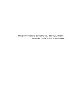
Fig. 7. Basic architecture of the control system of the Robotenis platform.

The results above are used in real time to control each joint independently. The joint
controller is based in a classical computed-torque controller plus a PD controller (Santibañez
and Kelly 2001). The objective of the computed-torque controller is to Feedback a signal that
cancels the effects of gravity, friction, the manipulator inertia tensor, and Coriolis and
centrifugal force, see in Fig. 7.

3.4 Trajectory planner
The structure of the visual controller of the Robotenis system is called dynamic position-
based on a look-and-move structure (Corke 1993). The above structure is formed of two
intertwined control loops: the first is faster and makes use of joints feedback, the second is
external to the first one and makes use of the visual information feedback, see in Fig. 7.
Once that the visual control loop analyzes the visual information then, this is sent to the
joint controller as a reference. In other words, in tracking tasks the desired next position is
calculated in the visual controller and the joint controller forces to the robot to reach it. Two
control loops are incorporated in the Robotenis system: the joint loop is calculated each 0.5
ms; at this point dynamical model, kinematical model and PD action are retrofitted. The
external loop is calculated each 8.33 ms and it was mentioned that uses the visual data. As
the internal loop is faster than the external, a trajectory planner is designed in order to
accomplish different objectives: The first objective is to make smooth trajectories in order to
avoid abrupt movements of the robot elements. The trajectory planner has to guarantee that
the positions and its following 3 derivates are continuous curves (velocity, acceleration and
jerk). The second objective is to guarantee that the actuators of the robot are not saturated
and that the robot specifications are not exceeded, the robot limits are: MVS= maximum
allowed velocity, MAS= maximum allowed acceleration and MJS= maximum allowed jerk
(maximum capabilities of the robot are taken from the end effector). In the Robotenis system
maximum capabilities are: 




, 




, and 



.





Robot
Vision
system
Visual
controller
Inverse and
direct
Kinematics
PD Joint
Controller
End effector
Trajectory
planner
Inverse
Dynamics


































 




NewvisualServoingcontrolstrategiesintrackingtasksusingaPKM 135
 
 


 
= 2
i
P h H ac c
x i i
P
x


 
  

ǡ ൌͳǡʹǡ͵
 
 
 
=2
i

P h H ac s
y
i i
P
y
 
 
 
  
 
  
ǡ ൌͳǡʹǡ͵
 
 
= 2
i
P as
z i
P
z

 


ǡ ൌͳǡʹǡ͵
       
1
= 2
1 1 1 1
1

a c P c P h H s P c
x y z
   

 
 
 
   
 
 
  
 

߲߁
ଶ
߲ߠ
ଶ
ൌ
߲߁
ଷ
߲ߠ
ଷ
ൌͲ
       
2
= 2
2 2 2 2
2
a c P c P h H s P c
x y z

   

 
 
 
   
 
 
  
 

߲߁
ଵ
߲ߠ
ଵ
ൌ
߲߁
ଷ
߲ߠ
ଷ
ൌͲ
       
3
= 2
3 3 3 3
3
a c P c P h H s P c
x y z
   


 
 
 
   
 
 
  
 

߲߁
ଵ
߲ߠ
ଵ
ൌ
߲߁
ଶ
߲ߠ
ଶ
ൌͲ

Once we have the derivatives above, they are substituted into equation (44) and the
Lagrangian multipliers are calculated. Thus for݆ൌͳǡʹǡ͵.



 





















        
 
           
 
 
 
 
 
 

2
1 1 1 2 2 2 3 3 3
3
P h H a c c P h H a c c P h H a c c

x x x
m m p F
p
b x P x
 
 
   


 
 


 
        
 
     
           
     
 
     
 
 
 
 
 

2
1 1 1 2 2 2 3 3 3
3

P h H a c s P h H a c s P h H a c s
y y y
m m p F
p
b y P y


 








     
   
 
         
   
 
 
   

2 3 3
1 1 2 2 3 3
P a s P a s P a s m m p g m m F
z z z
p

b z
p
b P z
(50)

Note that ܨ
௉௫
ǡܨ
௉௬
and ܨ
௉௭
are the componentsሺܳ
௝
ǡ݆ൌͳǡʹǡ͵ሻ of an external force that is
applied on the mobile platform. Once that the Lagrange multipliers are calculated the (45) is
solved (where݆ൌͶǡͷǡ͸) and for the actuator torquesሺ߬
௖௞
ൌܳ
௞ାଷ
ǡ݇ൌͳǡʹǡ͵ሻ.



 
         
2 2
2
1 1 1 1 1 1 1 1
m a I m a m m g a c a P c P s h H s P c
c a b a b x y z

       


 
         
 


 





 
         
2 2
2
2 2 2 2 2 2 2 2
m a I m a m m g a c a P c P s h H s P c
c a b a b x y z
       


 
         
 


 






           
2 2
2
3 3 3 3 3 3 3 3
m a I m a m m g a c a P c P s h H s P c
c a b a b x y z
       
 
 
         
 
 
 
 

(51)
Fig. 7. Basic architecture of the control system of the Robotenis platform.

The results above are used in real time to control each joint independently. The joint
controller is based in a classical computed-torque controller plus a PD controller (Santibañez
and Kelly 2001). The objective of the computed-torque controller is to Feedback a signal that
cancels the effects of gravity, friction, the manipulator inertia tensor, and Coriolis and
centrifugal force, see in Fig. 7.

3.4 Trajectory planner

The structure of the visual controller of the Robotenis system is called dynamic position-
based on a look-and-move structure (Corke 1993). The above structure is formed of two
intertwined control loops: the first is faster and makes use of joints feedback, the second is
external to the first one and makes use of the visual information feedback, see in Fig. 7.
Once that the visual control loop analyzes the visual information then, this is sent to the
joint controller as a reference. In other words, in tracking tasks the desired next position is
calculated in the visual controller and the joint controller forces to the robot to reach it. Two
control loops are incorporated in the Robotenis system: the joint loop is calculated each 0.5
ms; at this point dynamical model, kinematical model and PD action are retrofitted. The
external loop is calculated each 8.33 ms and it was mentioned that uses the visual data. As
the internal loop is faster than the external, a trajectory planner is designed in order to
accomplish different objectives: The first objective is to make smooth trajectories in order to
avoid abrupt movements of the robot elements. The trajectory planner has to guarantee that
the positions and its following 3 derivates are continuous curves (velocity, acceleration and
jerk). The second objective is to guarantee that the actuators of the robot are not saturated
and that the robot specifications are not exceeded, the robot limits are: MVS= maximum
allowed velocity, MAS= maximum allowed acceleration and MJS= maximum allowed jerk
(maximum capabilities of the robot are taken from the end effector). In the Robotenis system
maximum capabilities are: 




, 




, and 




.





Robot
Vision
system
Visual
controller
Inverse and
direct
Kinematics
PD Joint
Controller
End effector
Trajectory
planner
Inverse
Dynamics

































 





MechatronicSystems,Simulation,ModellingandControl136
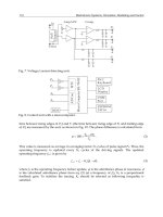
Fig. 8. Flowchart of the Trajectory planner.

And the third objective is to guarantee that the robot is in prepared to receive the next
reference, in this point the trajectory planner imposes a cero jerk and acceleration at the end
of each trajectory. In order to design the trajectory planner it has to be considered the system
constrains, the maximum jerk and maximum acceleration. As a result we have that the jerk
can be characterized by:
     
s n s n
m a x
3
k
j e j e
T

   
 
(52)

Where 

is the maximum allowed jerk, , 











,  is the real time clock,


and 

represent the initial and final time of the trajectory. Supposing that the initial and
final acceleration are cero and by considering that the acceleration can be obtained from the
integral of the eq. (52) and that if 

 

then 





we have:

   
 
m a x
1 c o s
T j
a

 


 
(53)

By supposing that the initial velocity (

) is different of cero, the velocity can be obtained
from the convenient integral of the eq. (53).
A new 

is defined and the end effector
moves towards the new 

(considering
the maximum capabilities of the robot)
1

no
yes


is used in the
trajectory planner
and 

is reached.








 

 









 


 

























1









 

 






























 
 
2
s i n
m a x

T j
v v
i


 
 


  




(54)

Finally, supposing ݌
௜
as the initial position and integrating the eq. (54) to obtain the position:

 
 
3
2
s
1
m a x
2 2
2
T j

c o
p p T v
i i
 

 

 


    






(55)

We can see that the final position ݌
௙
is not defined in the eq. (55). ݌
௙
is obtained by
calculating not to exceed the maximum jerk and the maximum acceleration. From eq. (53)
the maximum acceleration can be calculated as:

 
 
m a x m a x

1 s
m a x 1 m a x
2
2
T j a
a c o j
T

 


   

(56)

The final position of the eq. (55) is reached when߬ൌͳ, thus substituting eq. (56) in eq. (55)
when߬ൌͳ, we have:

4
m a x
2
a
p p
T v
f
i i
T


  





(57)

By means of the eq. (57) ܽ
௠௔௫
can be calculated but in order to take into account the
maximum capabilities of the robot. Maximum capabilities of the robot are the maximum
speed, acceleration and jerk. By substituting the eq. (56) in (54) and operating, we can obtain
the maximum velocity in terms of the maximum acceleration and the initial velocity.
 
2
s i n
m a x m a x
m a x
2
1
T j T a
v v v
i i
 

 

 
    
 
 


(58)

Once we calculate a
m a x
from eq. (57) the next is comparing the maximum capabilities from
equations (56) and (58). If maximum capabilities are exceeded, then the final position of the
robot is calculated from the maximum capabilities and the sign of a
m a x
(note that in this
case the robot will not reach the desired final position). See the Fig. 8. The time history of
sample trajectories is described in the Fig. 9 (in order to plot in the same chart, all curves are
normalized). This figure describes when the necessary acceleration to achieve a target, is
bigger than the maximum allowed. It can be observed that the fifth target position (
83:3ms
)
is not reached but the psychical characteristics of the robot actuators are not exceeded.

NewvisualServoingcontrolstrategiesintrackingtasksusingaPKM 137
Fig. 8. Flowchart of the Trajectory planner.

And the third objective is to guarantee that the robot is in prepared to receive the next
reference, in this point the trajectory planner imposes a cero jerk and acceleration at the end
of each trajectory. In order to design the trajectory planner it has to be considered the system
constrains, the maximum jerk and maximum acceleration. As a result we have that the jerk
can be characterized by:
     
s n s n
m a x
3

k
j e j e
T

   
 
(52)

Where 

is the maximum allowed jerk, , 










,  is the real time clock,


and 

represent the initial and final time of the trajectory. Supposing that the initial and
final acceleration are cero and by considering that the acceleration can be obtained from the
integral of the eq. (52) and that if 


 

then 





we have:

   
 
m a x
1 c o s
T j
a

 

 
(53)

By supposing that the initial velocity (

) is different of cero, the velocity can be obtained
from the convenient integral of the eq. (53).
A new 

is defined and the end effector
moves towards the new 


(considering
the maximum capabilities of the robot)
1

no
yes


is used in the
trajectory planner
and 

is reached.







 

 










 


 

























1









 

 






























 
 
2
s i n
m a x
T j
v v
i
 
 
 
 
  
 
 
(54)

Finally, supposing ݌
௜
as the initial position and integrating the eq. (54) to obtain the position:

 
 
3
2
s
1
m a x
2 2
2
T j
c o
p p T v
i i
 

 

 
 
    
 
 
 
(55)

We can see that the final position ݌

௙
is not defined in the eq. (55). ݌
௙
is obtained by
calculating not to exceed the maximum jerk and the maximum acceleration. From eq. (53)
the maximum acceleration can be calculated as:

 
 
m a x m a x
1 s
m a x 1 m a x
2
2
T j a
a c o j
T

 


   

(56)

The final position of the eq. (55) is reached when߬ൌͳ, thus substituting eq. (56) in eq. (55)
when߬ൌͳ, we have:

4
m a x

2
a
p p
T v
f
i i
T
 
  
 
 
(57)

By means of the eq. (57) ܽ
௠௔௫
can be calculated but in order to take into account the
maximum capabilities of the robot. Maximum capabilities of the robot are the maximum
speed, acceleration and jerk. By substituting the eq. (56) in (54) and operating, we can obtain
the maximum velocity in terms of the maximum acceleration and the initial velocity.
 
2
s i n
m a x m a x
m a x
2
1
T j T a
v v v
i i
 


 

 
    
 
 

(58)

Once we calculate a
m a x
from eq. (57) the next is comparing the maximum capabilities from
equations (56) and (58). If maximum capabilities are exceeded, then the final position of the
robot is calculated from the maximum capabilities and the sign of a
m a x
(note that in this
case the robot will not reach the desired final position). See the Fig. 8. The time history of
sample trajectories is described in the Fig. 9 (in order to plot in the same chart, all curves are
normalized). This figure describes when the necessary acceleration to achieve a target, is
bigger than the maximum allowed. It can be observed that the fifth target position (
83:3ms
)
is not reached but the psychical characteristics of the robot actuators are not exceeded.

MechatronicSystems,Simulation,ModellingandControl138
Fi
g
n
o

4.


C
o
w
o
re
s
ca
m
co
o
Tr
a
ki
n
is
c
an
its

Al
H
u
ba
20
0
ob

p
o
co
n
ca
s
ef
f
g
. 9. Example of
t
o
t reached (whe
n


Description o
f
o
ordinated s
y
ste
m
o
rd coordinate s
y
s
pectivel
y
. Othe

r
m
era coordinate
o
rdinate syste
m
a
nsformation m
a
n
ematical model
c
alculated b
y
m
e
d b
y
means of t
h

calculation requ
i
thou
g
h there ar
u
tchinson, Visua
l
sed in position

0
6). Schematic c
o
tained thou
g
h t
h
o
sition (

n
siderin
g
when
s
e). Once the er
r
f
ector. B
y
means
o
t
he time respons
e
t = 83:3ms
) but
r
f
the visual co

n
m
s are shown in
y
stem, the end-e
f
r
notations defi
n
system,
w
p
e


rep
r
m
.
w
p
e
is obta
i
a
trices are
w
R
e

and
e
R
c
is obtai
e
ans of the mass
c
h
e diameter of th
e
i
res sub-pixel pr
e
e advanced co
n
l
servo control. I
(Chaumette and

o
ntrol can be ap
p
h
e difference bet
w
). In the prese
n
desired position

r
or is obtained,
t
o
f the tra
j
ector
y

p
e
of the tra
j
ector
y
r
obot capabilitie
s
n
troller.
the Fig. 10 and
a
f
fector robot s
y
s
n
ed are:
c
p

b
rep
r
r
esents the positi
ined by mean
s
,
w
R
c
and
e
R
ned from the ca
m
c
enter of the pro
j
e
ball ( ). Dia
m
e
cisio
n
technique
s
n
trollers that ha
v

I Advanced app
r

Hutchinson, Vi
s
p
reciated in the
F
w
een the referen
c
n
t article the co
n

is fixed (static
c
t
he controller ca
l
p
lanner and the
J
y
planner, note t
h
s
are not exceede
d
a

re
§
w
,
§
e
, and
§
tem and the ca
m
r
esents the posi
t
on of the robot e
n
s
of the direc
R
c
where
w
R
e

i
m
era calibratio
n
.
j

ection of the bal
l
m
eter of the ball is

s
.
v
e been propos
e
r
oaches 2007), t
h
s
ual servo contr
o
F
ig. 7 and Fig. 1
c
e position (
n
trol si
g
nal is o
c
ase) and when
i
l
culates the desi
r

J
acobian matrix,
a
h
at the target pos
i
d
.
§
c
which repres
e
m
era coordinate
s
t
ion of the ball
n
d effector in th
e
t kinematical
m
i
s calculated fr
o
The position of t
h
l
on the image (

principally criti
c
e
d b
y
(Chaumet
t
h
e controller sele
c
o
l. I. Basic appr
o
0, the error func
) and the me
a
btained as a re
s
i
t is variable (d
y
r
ed velocit
y
of t
h
a
ll the
j
oint moti

o

i
tion is
e
nt the
sy
stem
in the
e
word
m
odel.
o
m the
h
e ball
)
c
al and
t
e and
c
ted is
o
aches
c
tion is
a
sured

s
ult of
y
namic
h
e end
o
ns are
calculated. Signals are supposed as known in the instant ݇ܶ, where ܶ is the sample time in
the visual control loop (in order to simplify we suppose ݇ܶ as ݇).


Fig. 10. Coordinated systems that are considered in the controller.

4.1 Static case
In the Fig. 7 can be observed that the position error can be expressed as follows:

 
*
( )
c c
e k p p k
b b
 
(59)

In this section ݌
௖
௕
כ

ሺ
݇
ሻ
is the desired position of the ball in the camera coordinate system and
in this section is considered as constant and known. ݌
௖
௕
ሺ
݇
ሻ
is the position of the ball in the
camera coordinate system. Thus, by considering the position in the word coordinate system:
   


( )
c c w w
p
k R p k p k
b w b c
 
(60)

If (60) is substituted into (59) then we obtain:
*
( ) ( ( ) ( ) )
c c w w
e k p R p k p k
b w b c
  

(61)

The system (robot) is supposed stable and in order to guarantee that the error will decrease
exponentially we choose:
c

C
Y
( , , )
b b b
X
Y Z
c
b
p
w
b
p
w
c
p
C
X
C
Z
w

w
Z
w

X
w
Y
NewvisualServoingcontrolstrategiesintrackingtasksusingaPKM 139
Fi
g
n
o

4.


C
o
w
o
re
s
ca
m
co
o
Tr
a
ki
n
is
c
an
its

Al
H
u
ba
20
0
ob
p
o
co
n
ca
s
ef
f
g
. 9. Example of
t
o
t reached (whe
n


Description o
f
o
ordinated s
y
ste

m
o
rd coordinate s
y
s
pectivel
y
. Othe
r
m
era coordinate
o
rdinate s
y
ste
m
a
nsformation m
a
n
ematical model
c
alculated b
y
m
e
d b
y
means of t
h

calculation requ
i
thou
g
h there ar
u
tchinson, Visua
l
sed in position
0
6). Schematic c
o
tained thou
g
h t
h
o
sition (

n
siderin
g
when
s
e). Once the er
r
f
ector. B
y

means
o
t
he time respons
e
t = 83:3ms
) but
r
f
the visual co
n
m
s are shown in
y
stem, the end-e
f
r
notations defi
n
system,
w
p
e


rep
r
m
.
w

p
e
is obta
i
a
trices are
w
R
e

and
e
R
c
is obtai
e
ans of the mass
c
h
e diameter of th
e
i
res sub-pixel pr
e
e advanced co
n
l
servo control. I
(Chaumette and

o
ntrol can be ap
p
h
e difference bet
w
). In the prese
n
desired position

r
or is obtained,
t
o
f the tra
j
ector
y

p
e
of the tra
j
ector
y
r
obot capabilitie
s
n
troller.

the Fig. 10 and
a
f
fector robot s
y
s
n
ed are:
c
p
b
rep
r
r
esents the positi
i
ned b
y
mean
s
,
w
R
c
and
e
R
ned from the ca
m
c

enter of the pro
j
e
ball ( ). Dia
m
e
cisio
n
technique
s
n
trollers that ha
v
I Advanced app
r

Hutchinson, Vi
s
p
reciated in the
F
w
een the referen
c
n
t article the co
n

is fixed (static
c

t
he controller ca
l
p
lanner and the
J
y
planner, note t
h
s
are not exceede
d
a
re
§
w
,
§
e
, and
§
tem and the ca
m
r
esents the posi
t
on of the robot e
n
s
of the direc

R
c
where
w
R
e

i
m
era calibratio
n
.
j
ection of the bal
l
m
eter of the ball is

s
.
v
e been propos
e
r
oaches 2007), t
h
s
ual servo contr
o
F

i
g
. 7 and Fig. 1
c
e position (
n
trol si
g
nal is o
c
ase) and when
i
l
culates the desi
r
J
acobian matrix,
a
h
at the target pos
i
d
.
§
c
which repres
e
m
era coordinate
s

t
ion of the ball
n
d effector in th
e
t kinematical
m
i
s calculated fr
o
The position of t
h
l
on the image (

principally criti
c
e
d b
y
(Chaumet
t
h
e controller sele
c
o
l. I. Basic appr
o
0, the error fun
c

) and the me
a
btained as a re
s
i
t is variable (d
y
r
ed velocit
y
of t
h
a
ll the
j
oint moti
o

i
tion is
e
nt the
sy
stem
in the
e
word
m
odel.
o

m the
h
e ball
)
c
al and
t
e and
c
ted is
o
aches
c
tion is
a
sured
s
ult of
y
namic
h
e end
o
ns are
calculated. Signals are supposed as known in the instant ݇ܶ, where ܶ is the sample time in
the visual control loop (in order to simplify we suppose ݇ܶ as ݇).


Fig. 10. Coordinated systems that are considered in the controller.

4.1 Static case
In the Fig. 7 can be observed that the position error can be expressed as follows:

 
*
( )
c c
e k p p k
b b
 
(59)

In this section ݌
௖
௕
כ
ሺ
݇
ሻ
is the desired position of the ball in the camera coordinate system and
in this section is considered as constant and known. ݌
௖
௕
ሺ
݇
ሻ
is the position of the ball in the
camera coordinate system. Thus, by considering the position in the word coordinate system:
   



( )
c c w w
p
k R p k p k
b w b c
 
(60)

If (60) is substituted into (59) then we obtain:
*
( ) ( ( ) ( ) )
c c w w
e k p R p k p k
b w b c
  
(61)

The system (robot) is supposed stable and in order to guarantee that the error will decrease
exponentially we choose:
c

C
Y
( , , )
b b b
X
Y Z
c
b

p
w
b
p
w
c
p
C
X
C
Z
w

w
Z
w
X
w
Y
MechatronicSystems,Simulation,ModellingandControl140




0e k e k w h e r e
 
 

(62)

Deriving (60) and supposing that 



and 


are constant, we obtain:
   


( )
c w w
e k R v k v k
w b c
  

(63)

Substituting (61)and (63)into (62), we obtain:
   


*
( )
w w c T c c
v k v k R p p k
c b w b b

  

(64)

Where 


and 


represent the camera and ball velocities (in the word coordinate
system) respectively. Since  





 







the control law can be expressed as:
     
*w c T c c
u k v k R p p k
b w b b

 

  
 
 
(65)

The equation (65) is composed by two components: a component which predicts the
position of the ball ( 





) and the other contains the tracking error ( 



 





).The
ideal control scheme (65) requires a perfect knowledge of all its components, which is not
possible, a more realistic approach consist in generalizing the previous control as
     
*
ˆ ˆ ˆ
( )
w w c T c c

u k v k v k R p p k
c b w b b

 
   
 
 
(66)

Where, the estimated variables are represented by the carets. A fundamental aspect in the
performing of the visual controller is the adjustment of, therefore  will be calculated in
the less number of sample time periods and will consider the system limitations. This
algorithm is based in the future positions of the camera and the ball; this lets to the robot
reaching the control objective ( 





 



). By supposing “n” small, the future position
(in the  instant) of the ball and the camera in the word coordinate system are:
   
ˆ ˆ ˆ
w w w
p
k n p v k n T

b b b
  

(67)
   
w w w
p
k n p v k n T
c c c
  

(68)

Where  is the visual sample time period. As was mentioned, the control
objective is to reach the target position in the shorter time as be possible. By taking into
account eq. (61), the estimated value 


and by considering that the error is cero  in
the instant, we have:

   
*
ˆ
0
c c w w
p R p k n p k n
b w b c
 
    

 
 

(69)
Substituting (67) and (68) into (69), we obtain (70).

       
*
ˆ ˆ
c c w w w w
p
R
p
k v k n T
p
k v k n T
b w b b c c


   





(70)

Taking into account that the estimate of the velocity of the ball is:

   



ˆ ˆ
( )
c c w w
p
k R
p
k
p
k
b w b c
 

(71)

Then the control law can be expressed as:

       
1
*
ˆ ˆ ˆ
w w c T c c
u k v k v k R
p p
k
c b w b b
nT



   





(72)

If (66) and (72) are compared, we can obtain the λ parameter as:

1
nT



(73)

The equation (73) gives a criterion for adjust  as a function of the number of samples
required  for reaching the control target. The visual control architecture proposed above
does not consider the physical limitations of the system such as delays and the maximum
operation of the components. If we consider that the visual information ( 





) has a
delay of 2 sampling times () with respect to the joint information, then at an
instant, the future position of the ball can be:

   
 
 
ˆ ˆ ˆ
w w w
p
k n p k r v k r T n r
b b b

    

(74)

The future position of the camera in the word coordinate system is given by (68). Using the
(74) is possible to adjust the  for the control law by considering the following aspect:
-The wished velocity of the end effector is represented by (72). In physical systems the
maximal velocity is necessary to be limited. In our system the maximal velocity of each joint
is taken into account to calculate. Value of depends of the instant position of the end
effector. Therefore through the robot jacobian is possible to know the velocity that requires
moving each joint and the value of  is adjusted to me more constrained joint (maximal
velocity of the joint).

4.2 Dynamic case
Static case is useful when the distance between the ball and the camera must be fixed but in
future tasks it is desirable that this distance change in real time. In this section, in order to
carry out above task a dynamic visual controller is designed. This controller receives two
parameters as are the target position and the target velocity. By means of above parameters
the robot can be able to carry out several tasks as are: catching, touching or hitting objects
NewvisualServoingcontrolstrategiesintrackingtasksusingaPKM 141





0e k e k w h e r e
 

 

(62)

Deriving (60) and supposing that 



and 


are constant, we obtain:
   


( )
c w w
e k R v k v k
w b c
  

(63)

Substituting (61)and (63)into (62), we obtain:

   


*
( )
w w c T c c
v k v k R p p k
c b w b b

  
(64)

Where 


and 


represent the camera and ball velocities (in the word coordinate
system) respectively. Since  





 








the control law can be expressed as:
     
*w c T c c
u k v k R p p k
b w b b



  




(65)

The equation (65) is composed by two components: a component which predicts the
position of the ball ( 





) and the other contains the tracking error ( 



 






).The
ideal control scheme (65) requires a perfect knowledge of all its components, which is not
possible, a more realistic approach consist in generalizing the previous control as
     
*
ˆ ˆ ˆ
( )
w w c T c c
u k v k v k R p p k
c b w b b



   




(66)

Where, the estimated variables are represented by the carets. A fundamental aspect in the
performing of the visual controller is the adjustment of, therefore  will be calculated in
the less number of sample time periods and will consider the system limitations. This
algorithm is based in the future positions of the camera and the ball; this lets to the robot
reaching the control objective ( 






 



). By supposing “n” small, the future position
(in the  instant) of the ball and the camera in the word coordinate system are:
   
ˆ ˆ ˆ
w w w
p
k n p v k n T
b b b
  

(67)
   
w w w
p
k n p v k n T
c c c
  

(68)

Where  is the visual sample time period. As was mentioned, the control

objective is to reach the target position in the shorter time as be possible. By taking into
account eq. (61), the estimated value 


and by considering that the error is cero  in
the instant, we have:

   
*
ˆ
0
c c w w
p R p k n p k n
b w b c



   





(69)
Substituting (67) and (68) into (69), we obtain (70).

       
*
ˆ ˆ
c c w w w w

p
R
p
k v k n T
p
k v k n T
b w b b c c
 
   
 
 

(70)

Taking into account that the estimate of the velocity of the ball is:

   


ˆ ˆ
( )
c c w w
p
k R
p
k
p
k
b w b c
 

(71)

Then the control law can be expressed as:

       
1
*
ˆ ˆ ˆ
w w c T c c
u k v k v k R
p p
k
c b w b b
nT
 
   
 
 

(72)

If (66) and (72) are compared, we can obtain the λ parameter as:

1
nT



(73)

The equation (73) gives a criterion for adjust  as a function of the number of samples
required  for reaching the control target. The visual control architecture proposed above
does not consider the physical limitations of the system such as delays and the maximum
operation of the components. If we consider that the visual information ( 





) has a
delay of 2 sampling times () with respect to the joint information, then at an
instant, the future position of the ball can be:

   
 
 
ˆ ˆ ˆ
w w w
p
k n p k r v k r T n r
b b b
     

(74)

The future position of the camera in the word coordinate system is given by (68). Using the
(74) is possible to adjust the  for the control law by considering the following aspect:
-The wished velocity of the end effector is represented by (72). In physical systems the
maximal velocity is necessary to be limited. In our system the maximal velocity of each joint

is taken into account to calculate. Value of depends of the instant position of the end
effector. Therefore through the robot jacobian is possible to know the velocity that requires
moving each joint and the value of  is adjusted to me more constrained joint (maximal
velocity of the joint).

4.2 Dynamic case
Static case is useful when the distance between the ball and the camera must be fixed but in
future tasks it is desirable that this distance change in real time. In this section, in order to
carry out above task a dynamic visual controller is designed. This controller receives two
parameters as are the target position and the target velocity. By means of above parameters
the robot can be able to carry out several tasks as are: catching, touching or hitting objects
MechatronicSystems,Simulation,ModellingandControl142
that are static or while are moving. In this article the principal objective is the robot hits the
ball in a specific point and with a specific velocity. In this section 



is no constant and







is considered instead, 







is the relative target velocity between the ball and the
camera and the error between the target and measured position is expressed as:

     
*c c
e k
p
k
p
k
b b
 

(75)

Substituting (60) in (75) and supposing that only 


is constant, we obtain its derivate as:

       


*c c w w
e k v k R v k v k
b w b c
  


(76)

Where 






is considered as the target velocity to carry out the task. By following a
similar analysis that in the static case, our control law would be:

         


 
* *
ˆ ˆ ˆ
w w c T c c c
u k v k v k R
p
k
p
k v k
c b w b b b

 
    
 

 

(77)

Where 





and 





are estimated and are the position and the velocity of the ball.
Just as to the static case, from the eq. (61) is calculated if the error is cero in .

     


*
ˆ
0
c c w w
p
k n R
p
k n

p
k n
b w b c
     

(78)

Substituting (67) and (68) in (78) and taking into account the approximation:

 
   
* * *c c c
p
k n
p
k nT v k
b b b
  

(79)

Is possible to obtain:
           


* *
ˆ ˆ
0
c c c w w w w
p

k n T v k R
p
k nT v k
p
k n T v k
b b w b b c c
     

(80)

Taking into account the eq. (71), the control law can be obtained as:

         


 
1
* *
ˆ ˆ ˆ
w w c T c c c
u k v k v k R p k p k v k
c b w b b b
n T
 
    
 
 

(81)

From eq. (77) it can be observed that  can be 


where “” is “small enough”.

4.3 Stability and errors influence
By means of Lyapunov analysis is possible to probe the system stability; it can be
demonstrated that the error converges to zero if ideal conditions are considered; otherwise it
can be probed that the error will be bounded under the influence of the estimation errors
and non modelled dynamics. We choose a Lyapunov function as:

   
1
2
T
V e k e k

(82)
   
T
V e k e k



(83)

If the error behavior is described by the eq. (62) then

( ) ( ) 0
T

V e k e k


 


(84)

The eq. (84) implies 



 when  and this is only true if



 





. Note that
above is not true due to estimations ( 





 






) and dynamics that are not modelled.
Above errors are expressed in



and is more realistic to consider (



 





):

       
ˆ
w w
u k v k v k k
c c

  

(85)

By considering the estimated velocity of the ball ( 


) in eq. (76) and substituting the eq.
(85) is possible to obtain:

         
*c c w w
e k v k R v k v k k
b w b c



   






(86)

Note that estimate errors are already included in. Consequently the value of 






is:

       


 
* *w w c T c c c
v k v k R
p
k
p
k v k
c b w b b b



   





(87)

Substituting eq. (87) in (86):
           


   
* * *c c w w c T c c c

e k v k R v k v k R
p
k
p
k v k k
b w b b w b b b
 


 
      


 
 




(88)

Operating in order to simplify:

         


     
* * *c c c c c c
e k v k v k p k p k R k R k e k
b b b b w w

   
      


(89)

Taking into account the Lyapunov function in eq. (82):

           
T T T c
V e k e k e k e k e k R k
w
 
  



(90)

Thus, by considering 

we have that the following condition has to be satisfied:
NewvisualServoingcontrolstrategiesintrackingtasksusingaPKM 143
that are static or while are moving. In this article the principal objective is the robot hits the
ball in a specific point and with a specific velocity. In this section 



is no constant and








is considered instead, 






is the relative target velocity between the ball and the
camera and the error between the target and measured position is expressed as:

     
*c c
e k
p
k
p
k
b b
 

(75)

Substituting (60) in (75) and supposing that only 



is constant, we obtain its derivate as:

       


*c c w w
e k v k R v k v k
b w b c
  


(76)

Where 






is considered as the target velocity to carry out the task. By following a
similar analysis that in the static case, our control law would be:

         


 
* *
ˆ ˆ ˆ

w w c T c c c
u k v k v k R
p
k
p
k v k
c b w b b b



    





(77)

Where 





and 






are estimated and are the position and the velocity of the ball.
Just as to the static case, from the eq. (61) is calculated if the error is cero in .

     


*
ˆ
0
c c w w
p
k n R
p
k n
p
k n
b w b c
     

(78)

Substituting (67) and (68) in (78) and taking into account the approximation:

 
   
* * *c c c
p
k n
p
k nT v k

b b b
  

(79)

Is possible to obtain:
           


* *
ˆ ˆ
0
c c c w w w w
p
k n T v k R
p
k nT v k
p
k n T v k
b b w b b c c
     

(80)

Taking into account the eq. (71), the control law can be obtained as:

         


 

1
* *
ˆ ˆ ˆ
w w c T c c c
u k v k v k R p k p k v k
c b w b b b
n T
 
    
 
 

(81)

From eq. (77) it can be observed that  can be 


where “” is “small enough”.

4.3 Stability and errors influence
By means of Lyapunov analysis is possible to probe the system stability; it can be
demonstrated that the error converges to zero if ideal conditions are considered; otherwise it
can be probed that the error will be bounded under the influence of the estimation errors
and non modelled dynamics. We choose a Lyapunov function as:

   
1
2
T
V e k e k

(82)
   
T
V e k e k



(83)

If the error behavior is described by the eq. (62) then

( ) ( ) 0
T
V e k e k

 


(84)

The eq. (84) implies 



 when  and this is only true if



 






. Note that
above is not true due to estimations ( 





 





) and dynamics that are not modelled.
Above errors are expressed in



and is more realistic to consider (



 






):

       
ˆ
w w
u k v k v k k
c c

  

(85)

By considering the estimated velocity of the ball ( 


) in eq. (76) and substituting the eq.
(85) is possible to obtain:

         
*c c w w
e k v k R v k v k k
b w b c

 
   
 
 



(86)

Note that estimate errors are already included in. Consequently the value of 





is:

       


 
* *w w c T c c c
v k v k R
p
k
p
k v k
c b w b b b

 
   
 
 

(87)

Substituting eq. (87) in (86):
           


   
* * *c c w w c T c c c
e k v k R v k v k R
p
k
p
k v k k
b w b b w b b b
 
 
 
      
 
 
 
 


(88)

Operating in order to simplify:

         



     
* * *c c c c c c
e k v k v k p k p k R k R k e k
b b b b w w
   
      


(89)

Taking into account the Lyapunov function in eq. (82):

           
T T T c
V e k e k e k e k e k R k
w
 
  



(90)

Thus, by considering 

we have that the following condition has to be satisfied:
MechatronicSystems,Simulation,ModellingandControl144
e





(91)

Above means that if the error is bigger that
ԡ
ఘ
ԡ
ఒ
then the error will decrease but it will not
tend to cero, finally the error is bounded by.

e




(92)

By considering that errors from the estimation of the position and velocity are bigger that
errors from the system dynamics, then ߩ
ሺ
݇
ሻ
can be obtained if we replace (77) and (87) in
(85)
         


ˆ ˆ

w w c T c c
k v k v k R
p
k
p
k
b b w b b
 
   

(93)

5. Conclusions and future works

In this work the full architecture of the Robotenis system and a novel structure of visual
control were shown in detail. In this article no results are shown but the more important
elements to control and simulate the robot and visual controller were described. Two
kinematic models were described in order to obtain two different jacobians were each
jacobian is used in different tasks: the System simulator and the real time controller. By
means of the condition index of the robot jacobians some singularities of the robot are
obtained. In real time tasks the above solution and the condition index of the second
jacobian are utilized to bound the work space and avoid singularities, in this work if some
point forms part or is near of a singularity then the robot stop the end effector movement
and waits to the next target point.
Inverse dynamics of the robot is obtained by means of the Lagrange multipliers. The inverse
dynamics is used in a non linear feed forward in order to improve the PD joint controller.
Although improvement of the behaviour of the robot in notorious, in future works is
important to measure how the behaviour is modified when the dynamics fed forward is
added and when is not.
The trajectory planner is added with two principal objectives: the trajectory planner assures

that the robot capabilities are not exceeded and assures that the robot moves softly. The
trajectory planner takes into account the movements of the end effector, this consideration
has drawbacks: the principal is that the maximum end-effector capabilities are not
necessarily the maximum joint capabilities, depends on the end effector position. Above
drawbacks suggest redesigning the trajectory planner in order to apply to the joint space,
this as another future work.
Above elements are used in the visual controller and the robot controller has to satisfied the
visual controller requirements. Thanks to the joint controller the robot is supposed stable
and its response is considered faster than the visual system. Two cases are presented in this
paper: the static case that is exposed in other works and some results and videos are shown,
the another controller is called the dynamic case. An objective of the system is to play ping
pong by itself and the controller of the dynamic case was specially designed in order to
reach this objective. The objective of the dynamic visual controller is to reach some point
with a desired velocity, this allows to the robot hit the ball with a desired speed and
direction. In order to hit the ball a special and partially spherical paddled is being designed
in order to give the desired effect to the ball. Finally the stability of visual controllers is
demonstrated by means of Lyapunov theory and the errors in the estimations are bounded.
As a future works, efforts of the vision group will be concentrated in the design of visual
controllers in order to improve the robot positioning and tracking.

6. References

Angel, L., J.M. Sebastian, R. Saltaren, R. Aracil, and J. Sanpedro. “Robotenis: optimal design
of a parallel robot with high performance.” IEEE/RSJ International Conference on,
(IROS 2005). IEEE Intelligent Robots and Systems, 2005. 2134- 2139.
Bonev, Ilian A., and Clément Gosselin. Fundamentals of Parallel Robots. Edited by Springer.
2009.
Chaumette, F., and S. Hutchinson. “Visual servo control. I. Basic approaches.” (Robotics &
Automation Magazine, IEEE) 13, no. 4 (December 2006): 82-90.
Chaumette, F., and S. Hutchinson. “Visual servo control. II Advanced approaches.”

(Robotics & Automation Magazine, IEEE) 14, no. 1 (March 2007): 109 – 118.
Clavel, Reymond. “DELTA: a fast robot with parallel geometry.” Sidney: 18th International
Symposium on Industrial Robot., 1988. 91–100.
Corke, Peter I. “Visual Control Of Robot Manipulators A Review.” In Visual Servoing: Real
Time Control of Robot Manipulators Based on Visual Sensory Feedback (Series in Robotics
and Automated Systems), edited by Hashimoto Kagami, 1-31, 300. World Scientific
Publishing Co Pte Ltd, 1993.
Corrochano, Eduardo Bayro, and Detlef Kähler. “Motor Algebra Approach for Computing
the Kinematics of Robot Manipulators.” Journal of Robotic Systems (Wiley
Periodicals), 2000: 495 - 516.
Davidson, J. K., and J. K. Hunt Davidson. Robots and Screw Theory: Applications of Kinematics
and Statics to Robotics . 1. Publisher: Oxford University Press, USA, 2004.
Kaneko, Makoto, Mitsuru Higashimori, Akio Namiki, and Masatoshi Ishikawa. “The 100G
Capturing Robot - Too Fast to See.” Edited by P. Dario and R. Chatila. Robotics
Research, 2005. 517–526.
Kragic, Danica, and Christensen Henrik I. “Advances in robot vision.” Vol. 52. Edited by
Elsevier. Robotics and Autonomous Systems, Science Direct, May 2005. 1-3.
Merlet, J.P. Parallel Robots (Solid Mechanics and Its Applications). Edited by Springer. 2006.
Morikawa, Sho, Taku Senoo, Akio Namiki, and Masatoshi Ishikawa. “Realtime collision
avoidance using a robot manipulator with light-weight small high-speed vision
systems.” Roma: Robotics and Automation IEEE International Conference on, April
2007. 794-797.
Oda, Naoki, Masahide Ito, and Masaaki Shibata. “Vision-based motion control for robotic
systems.” Vol. 4. no. 2. Edited by Hoboken. John Wiley. February 2009.
Santibañez, Victor, and Rafael. Kelly. “PD control with feedforward compensation for robot
manipulators: analysis and experimentation.” Robotica (Cambridge University
Press) 19, no. 1 (2001): 11-19.
NewvisualServoingcontrolstrategiesintrackingtasksusingaPKM 145
e





(91)

Above means that if the error is bigger that
ԡ
ఘ
ԡ
ఒ
then the error will decrease but it will not
tend to cero, finally the error is bounded by.

e




(92)

By considering that errors from the estimation of the position and velocity are bigger that
errors from the system dynamics, then ߩ
ሺ
݇
ሻ
can be obtained if we replace (77) and (87) in
(85)
         



ˆ ˆ
w w c T c c
k v k v k R
p
k
p
k
b b w b b
 
   

(93)

5. Conclusions and future works

In this work the full architecture of the Robotenis system and a novel structure of visual
control were shown in detail. In this article no results are shown but the more important
elements to control and simulate the robot and visual controller were described. Two
kinematic models were described in order to obtain two different jacobians were each
jacobian is used in different tasks: the System simulator and the real time controller. By
means of the condition index of the robot jacobians some singularities of the robot are
obtained. In real time tasks the above solution and the condition index of the second
jacobian are utilized to bound the work space and avoid singularities, in this work if some
point forms part or is near of a singularity then the robot stop the end effector movement
and waits to the next target point.
Inverse dynamics of the robot is obtained by means of the Lagrange multipliers. The inverse
dynamics is used in a non linear feed forward in order to improve the PD joint controller.
Although improvement of the behaviour of the robot in notorious, in future works is
important to measure how the behaviour is modified when the dynamics fed forward is
added and when is not.

The trajectory planner is added with two principal objectives: the trajectory planner assures
that the robot capabilities are not exceeded and assures that the robot moves softly. The
trajectory planner takes into account the movements of the end effector, this consideration
has drawbacks: the principal is that the maximum end-effector capabilities are not
necessarily the maximum joint capabilities, depends on the end effector position. Above
drawbacks suggest redesigning the trajectory planner in order to apply to the joint space,
this as another future work.
Above elements are used in the visual controller and the robot controller has to satisfied the
visual controller requirements. Thanks to the joint controller the robot is supposed stable
and its response is considered faster than the visual system. Two cases are presented in this
paper: the static case that is exposed in other works and some results and videos are shown,
the another controller is called the dynamic case. An objective of the system is to play ping
pong by itself and the controller of the dynamic case was specially designed in order to
reach this objective. The objective of the dynamic visual controller is to reach some point
with a desired velocity, this allows to the robot hit the ball with a desired speed and
direction. In order to hit the ball a special and partially spherical paddled is being designed
in order to give the desired effect to the ball. Finally the stability of visual controllers is
demonstrated by means of Lyapunov theory and the errors in the estimations are bounded.
As a future works, efforts of the vision group will be concentrated in the design of visual
controllers in order to improve the robot positioning and tracking.

6. References

Angel, L., J.M. Sebastian, R. Saltaren, R. Aracil, and J. Sanpedro. “Robotenis: optimal design
of a parallel robot with high performance.” IEEE/RSJ International Conference on,
(IROS 2005). IEEE Intelligent Robots and Systems, 2005. 2134- 2139.
Bonev, Ilian A., and Clément Gosselin. Fundamentals of Parallel Robots. Edited by Springer.
2009.
Chaumette, F., and S. Hutchinson. “Visual servo control. I. Basic approaches.” (Robotics &
Automation Magazine, IEEE) 13, no. 4 (December 2006): 82-90.

Chaumette, F., and S. Hutchinson. “Visual servo control. II Advanced approaches.”
(Robotics & Automation Magazine, IEEE) 14, no. 1 (March 2007): 109 – 118.
Clavel, Reymond. “DELTA: a fast robot with parallel geometry.” Sidney: 18th International
Symposium on Industrial Robot., 1988. 91–100.
Corke, Peter I. “Visual Control Of Robot Manipulators A Review.” In Visual Servoing: Real
Time Control of Robot Manipulators Based on Visual Sensory Feedback (Series in Robotics
and Automated Systems), edited by Hashimoto Kagami, 1-31, 300. World Scientific
Publishing Co Pte Ltd, 1993.
Corrochano, Eduardo Bayro, and Detlef Kähler. “Motor Algebra Approach for Computing
the Kinematics of Robot Manipulators.” Journal of Robotic Systems (Wiley
Periodicals), 2000: 495 - 516.
Davidson, J. K., and J. K. Hunt Davidson. Robots and Screw Theory: Applications of Kinematics
and Statics to Robotics . 1. Publisher: Oxford University Press, USA, 2004.
Kaneko, Makoto, Mitsuru Higashimori, Akio Namiki, and Masatoshi Ishikawa. “The 100G
Capturing Robot - Too Fast to See.” Edited by P. Dario and R. Chatila. Robotics
Research, 2005. 517–526.
Kragic, Danica, and Christensen Henrik I. “Advances in robot vision.” Vol. 52. Edited by
Elsevier. Robotics and Autonomous Systems, Science Direct, May 2005. 1-3.
Merlet, J.P. Parallel Robots (Solid Mechanics and Its Applications). Edited by Springer. 2006.
Morikawa, Sho, Taku Senoo, Akio Namiki, and Masatoshi Ishikawa. “Realtime collision
avoidance using a robot manipulator with light-weight small high-speed vision
systems.” Roma: Robotics and Automation IEEE International Conference on, April
2007. 794-797.
Oda, Naoki, Masahide Ito, and Masaaki Shibata. “Vision-based motion control for robotic
systems.” Vol. 4. no. 2. Edited by Hoboken. John Wiley. February 2009.
Santibañez, Victor, and Rafael. Kelly. “PD control with feedforward compensation for robot
manipulators: analysis and experimentation.” Robotica (Cambridge University
Press) 19, no. 1 (2001): 11-19.
MechatronicSystems,Simulation,ModellingandControl146
Sebastián, J.M., A. Traslosheros, L. Angel, F. Roberti, and R. Carelli. “Parallel robot high

speed objec tracking.” Chap. 3, by Image Analysis and recognition, edited by
Aurélio Campilho Mohamed Kamel, 295-306. Springer, 2007.
Senoo, T., A. Namiki, and M. Ishikawa. “High-speed batting using a multi-jointed
manipulator.” Vol. 2. Robotics and Automation, 2004. Proceedings. ICRA '04. 2004
IEEE International Conference on, 2004. 1191- 1196 .
Stamper, Richard Eugene, and Lung Wen Tsai. “A three Degree of freedom parallel
manipulator with only translational degrees of freedom.” PhD Thesis, Department
of mechanical engineering and institute for systems research, University of
Maryland, 1997, 211.
Stramigioli, Stefano, and Herman Bruyninckx. Geometry and Screw Theory for Robotics
(Tutorial). Tutorial, IEEE ICRA 2001, 2001.
Tsai, Lung Wen. Robot Analysis: The Mechanics of Serial and Parallel Manipulators. 1. Edited by
Wiley-Interscience. 1999.
Yoshikawa, Tsuneo. “Manipulability and Redundancy Ccontrol of Robotic Mechanisms.”
Vol. 2. Robotics and Automation. Proceedings. 1985 IEEE International Conference
on, March 1985. 1004- 1009.

NonlinearAdaptiveModelFollowingControlfora3-DOFModelHelicopter 147
NonlinearAdaptiveModelFollowingControlfora3-DOFModelHelicopter
MitsuakiIshitobiandMasatoshiNishi
0
Nonlinear Adaptive Model Following
Control for a 3-DOF Model Helicopter
Mitsuaki Ishitobi and Masatoshi Nishi
Department of Mechanical Systems Engineering
Kumamoto University
Japan
1. Introduction
Interest in designing feedback controllers for helicopters has increased over the last ten years
or so due to the important potential applications of this area of research. The main diffi-

culties in designing stable feedback controllers for helicopters arise from the nonlinearities
and couplings of the dynamics of these aircraft. To date, various efforts have been directed
to the development of effective nonlinear control strategies for helicopters (Sira-Ramirez et
al., 1994; Kaloust et al., 1997; Kutay et al., 2005; Avila et al., 2003). Sira-Ramirez et al. ap-
plied dynamical sliding mode control to the altitude stabilization of a nonlinear helicopter
model in vertical flight. Kaloust et al. developed a Lyapunov-based nonlinear robust control
scheme for application to helicopters in vertical flight mode. Avila et al. derived a nonlin-
ear 3-DOF
(degree-of-freedom) model as a reduced-order model for a 7-DOF helicopter, and
implemented a linearizing controller in an experimental system. Most of the existing results
have concerned flight regulation.
This study considers the two-input, two-output nonlinear model following control of a 3-DOF
model helicopter. Since the decoupling matrix is singular, a nonlinear structure algorithm
(Shima et al., 1997; Isurugi, 1990) is used to design the controller. Furthermore, since the model
dynamics are described linearly by unknown system parameters, a parameter identification
scheme is introduced in the closed-loop system.
Two parameter identification methods are discussed: The first method is based on the differ-
ential equation model. In experiments, it is found that this model has difficulties in obtaining
a good tracking control performance, due to the inaccuracy of the estimated velocity and ac-
celeration signals. The second parameter identification method is designed on the basis of a
dynamics model derived by applying integral operators to the differential equations express-
ing the system dynamics. Hence this identification algorithm requires neither velocity nor
acceleration signals. The experimental results for this second method show that it achieves
better tracking objectives, although the results still suffer from tracking errors. Finally, we
introduce additional terms into the equations of motion that express model uncertainties and
external disturbances. The resultant experimental data show that the method constructed
with the inclusion of these additional terms produces the best control performance.
9
MechatronicSystems,Simulation,ModellingandControl148
2. System Description

Consider the tandem rotor model helicopter of Quanser Consulting, Inc. shown in Figs. 1 and
2. The helicopter body is mounted at the end of an arm and is free to move about the elevation,
pitch and horizontal travel axes. Thus the helicopter has 3-DOF: the elevation ε, pitch θ and
travel φ angles, all of which are measured via optical encoders. Two DC motors attached to
propellers generate a driving force proportional to the voltage output of a controller.
Fig. 1. Overview of the present model helicopter.
Fig. 2. Notation.
The equations of motion about axes ε, θ and φ are expressed as
J
ε
¨
ε
= −

M
f
+ M
b

g
L
a
cos δ
a
cos
(
ε − δ
a
)
+

M
c
g
L
c
cos δ
c
cos
(
ε + δ
c
)
−
η
ε
˙
ε
+K
m
L
a

V
f
+ V
b

cos θ (1)
J
θ

¨
θ
= −M
f
g
L
h
cos δ
h
cos
(
θ − δ
h
)
+
M
b
g
L
h
cos δ
h
cos
(
θ + δ
h
)
−
η
θ

˙
θ
+ K
m
L
h

V
f
− V
b

(2)
J
φ
¨
φ
= −η
φ
˙
φ
− K
m
L
a

V
f
+ V
b


sin θ. (3)
A complete derivation of this model is presented in (Apkarian, 1998). The system dynamics
are expressed by the following highly nonlinear and coupled state variable equations
˙x
p
= f (x
p
) + [g
1
(x
p
), g
2
(x
p
)]u
p
(4)
where
x
p
= [x
p1
, x
p2
, x
p3
, x
p4

, x
p5
, x
p6
]
T
= [ε,
˙
ε, θ,
˙
θ, φ,
˙
φ]
T
u
p
= [u
p1
, u
p2
]
T
u
p1
= V
f
+ V
b
u
p2

= V
f
− V
b
f (x
p
) =








˙
ε
p
1
cos ε + p
2
sin ε + p
3
˙
ε
˙
θ
p
5
cos θ + p

6
sin θ + p
7
˙
θ
˙
φ
p
9
˙
φ








g
1
(x
p
) =
[
0, p
4
cos θ, 0, 0, 0, p
10
sin θ

]
T
g
2
(x
p
) =
[
0, 0, 0, p
8
, 0, 0
]
T
p
1
=

−(M
f
+ M
b
)gL
a
+ M
c
gL
c

J
ε

p
2
= −

(M
f
+ M
b
)gL
a
tan δ
a
+ M
c
gL
c
tan δ
c

J
ε
p
3
= −η
ε

J
ε
p
4

= K
m
L
a
/
J
ε
p
5
= (−M
f
+ M
b
)gL
h

J
θ
p
6
= −(M
f
+ M
b
)gL
h
tan δ
h

J

θ
p
7
= −η
θ

J
θ
p
8
= K
m
L
h

J
θ
p
9
= −η
φ

J
φ
p
10
= −K
m
L
a


J
φ
δ
a
= tan
−1
{(L
d
+ L
e
)/L
a
}
δ
c
= tan
−1
(L
d
/L
c
)
δ
h
= tan
−1
(L
e
/L

h
)
The notation employed above is defined as follows: V
f
, V
b
[V]: Voltage applied to the front
motor, voltage applied to the rear motor,
M
f
, M
b
[kg]: Mass of the front section of the helicopter, mass of the rear section,
M
c
[kg]: Mass of the counterbalance,
L
d
, L
c
, L
a
, L
e
, L
h
[m]: Distances OA, AB, AC, CD, DE=DF,
g [m/s
2
]: gravitational acceleration,

NonlinearAdaptiveModelFollowingControlfora3-DOFModelHelicopter 149
2. System Description
Consider the tandem rotor model helicopter of Quanser Consulting, Inc. shown in Figs. 1 and
2. The helicopter body is mounted at the end of an arm and is free to move about the elevation,
pitch and horizontal travel axes. Thus the helicopter has 3-DOF: the elevation ε, pitch θ and
travel φ angles, all of which are measured via optical encoders. Two DC motors attached to
propellers generate a driving force proportional to the voltage output of a controller.
Fig. 1. Overview of the present model helicopter.
Fig. 2. Notation.
The equations of motion about axes ε, θ and φ are expressed as
J
ε
¨
ε
= −

M
f
+ M
b

g
L
a
cos δ
a
cos
(
ε − δ
a

)
+
M
c
g
L
c
cos δ
c
cos
(
ε + δ
c
)
−
η
ε
˙
ε
+K
m
L
a

V
f
+ V
b

cos θ (1)

J
θ
¨
θ
= −M
f
g
L
h
cos δ
h
cos
(
θ − δ
h
)
+
M
b
g
L
h
cos δ
h
cos
(
θ + δ
h
)
−

η
θ
˙
θ
+ K
m
L
h

V
f
− V
b

(2)
J
φ
¨
φ
= −η
φ
˙
φ
− K
m
L
a

V
f

+ V
b

sin θ. (3)
A complete derivation of this model is presented in (Apkarian, 1998). The system dynamics
are expressed by the following highly nonlinear and coupled state variable equations
˙x
p
= f (x
p
) + [g
1
(x
p
), g
2
(x
p
)]u
p
(4)
where
x
p
= [x
p1
, x
p2
, x
p3

, x
p4
, x
p5
, x
p6
]
T
= [ε,
˙
ε, θ,
˙
θ, φ,
˙
φ]
T
u
p
= [u
p1
, u
p2
]
T
u
p1
= V
f
+ V
b

u
p2
= V
f
− V
b
f (x
p
) =








˙
ε
p
1
cos ε + p
2
sin ε + p
3
˙
ε
˙
θ
p

5
cos θ + p
6
sin θ + p
7
˙
θ
˙
φ
p
9
˙
φ








g
1
(x
p
) =
[
0, p
4
cos θ, 0, 0, 0, p

10
sin θ
]
T
g
2
(x
p
) =
[
0, 0, 0, p
8
, 0, 0
]
T
p
1
=

−(M
f
+ M
b
)gL
a
+ M
c
gL
c


J
ε
p
2
= −

(M
f
+ M
b
)gL
a
tan δ
a
+ M
c
gL
c
tan δ
c

J
ε
p
3
= −η
ε

J
ε

p
4
= K
m
L
a
/
J
ε
p
5
= (−M
f
+ M
b
)gL
h

J
θ
p
6
= −(M
f
+ M
b
)gL
h
tan δ
h


J
θ
p
7
= −η
θ

J
θ
p
8
= K
m
L
h

J
θ
p
9
= −η
φ

J
φ
p
10
= −K
m

L
a

J
φ
δ
a
= tan
−1
{(L
d
+ L
e
)/L
a
}
δ
c
= tan
−1
(L
d
/L
c
)
δ
h
= tan
−1
(L

e
/L
h
)
The notation employed above is defined as follows: V
f
, V
b
[V]: Voltage applied to the front
motor, voltage applied to the rear motor,
M
f
, M
b
[kg]: Mass of the front section of the helicopter, mass of the rear section,
M
c
[kg]: Mass of the counterbalance,
L
d
, L
c
, L
a
, L
e
, L
h
[m]: Distances OA, AB, AC, CD, DE=DF,
g [m/s

2
]: gravitational acceleration,
MechatronicSystems,Simulation,ModellingandControl150
J
ε
, J
θ
, J
φ
[kg·m
2
]: Moment of inertia about the elevation, pitch and travel axes,
η
ε
, η
θ
, η
φ
[kg·m
2
/s]: Coefficient of viscous friction about the elevation, pitch and travel axes.
The forces of the front and rear rotors are assumed to be F
f
=K
m
V
f
and F
b
=K

m
V
b
[N], re-
spectively, where K
m
[N/V] is a force constant. It may be noted that all the parameters
p
i
(i = 1 . . . 10) are constants. For the problem of the control of the position of the model
helicopter, two angles, the elevation ε and the travel φ angles, are selected as the outputs from
the three detected signals of the three angles. Hence, we have
y
p
= [ε, φ]
T
(5)
3. Nonlinear Model Following Control
3.1 Control system design
In this section, a nonlinear model following control system is designed for the 3-DOF model
helicopter described in the previous section.
First, the reference model is given as

˙x
M
= A
M
x
M
+ B

M
u
M
y
M
= C
M
x
M
(6)
where
x
M
= [x
M1
, x
M2
, x
M3
, x
M4
, x
M5
, x
M6
, x
M7
, x
M8
]

T
y
M
= [ε
M
, φ
M
]
T
u
M
= [u
M1
, u
M2
]
T
A
M
=

K
1
0
0 K
2

K
i
=





0 1 0 0
0 0 1 0
0 0 0 1
k
i1
k
i2
k
i3
k
i4




, i
= 1, 2
B
M
=

i
1
0
0 i
1


C
M
=

i
2
T
0
T
0
T
i
2
T

i
1
=




0
0
0
1





, i
2
=




1
0
0
0




From (4) and (6), the augmented state equation is defined as follows.
˙x
= f (x) + G(x)u (7)
where
x
= [x
T
p
, x
T
M
]
T
u = [u

T
p
, u
T
M
]
T
f (x) =

f
(x
p
)
A
M
x
M

G
(x) =

g
1
(x
p
) g
2
(x
p
) O

0 0 B
M

Here, we apply a nonlinear structure algorithm to design a model following controller (Shima
et al., 1997; Isurugi, 1990). New variables and parameters in the following algorithm are de-
fined below the input (19).
• Step 1
The tracking error vector is given by
e
=

e
1
e
2

=

x
M1
− x
p1
x
M5
− x
p5

(8)
Differentiating the tracking error (8) yields
˙e

=
∂e
∂x
{
f (x) + G(x)u
}
=

−x
p2
+ x
M2
−x
p6
+ x
M6

(9)
Since the inputs do not appear in (9), we proceed to step 2.
• Step 2
Differentiating (9) leads to
¨e
=
∂˙e
∂x
{
f (x) + G(x)u
}
(10)
=


r
1
(x)
−
p
9
x
p6
+ x
M7

+
[
B
u
(x), B
r
(x)
]
u (11)
where
B
u
(x) =

−p
4
cos x
p3

0
−p
10
sin x
p3
0

, B
r
(x) = O
From (11), the decoupling matrix B
u
(x) is obviously singular. Hence, this system is not de-
couplable by static state feedback. The equation (11) can be re-expressed as
¨
e
1
= r
1
(x) − p
4
cos x
p3
u
p1
(12)
¨
e
2
= −p

9
x
p6
+ x
M7
− p
10
sin x
p3
u
p1
(13)
then, by eliminating u
p1
from (13) using (12) under the assumption of u
p1
= 0, we obtain
¨
e
2
= −p
9
x
p6
+ x
M7
+
p
10
p

4
tan x
p3
(
¨
e
1
− r
1
(x)) (14)
NonlinearAdaptiveModelFollowingControlfora3-DOFModelHelicopter 151
J
ε
, J
θ
, J
φ
[kg·m
2
]: Moment of inertia about the elevation, pitch and travel axes,
η
ε
, η
θ
, η
φ
[kg·m
2
/s]: Coefficient of viscous friction about the elevation, pitch and travel axes.
The forces of the front and rear rotors are assumed to be F

f
=K
m
V
f
and F
b
=K
m
V
b
[N], re-
spectively, where K
m
[N/V] is a force constant. It may be noted that all the parameters
p
i
(i = 1 . . . 10) are constants. For the problem of the control of the position of the model
helicopter, two angles, the elevation ε and the travel φ angles, are selected as the outputs from
the three detected signals of the three angles. Hence, we have
y
p
= [ε, φ]
T
(5)
3. Nonlinear Model Following Control
3.1 Control system design
In this section, a nonlinear model following control system is designed for the 3-DOF model
helicopter described in the previous section.
First, the reference model is given as


˙x
M
= A
M
x
M
+ B
M
u
M
y
M
= C
M
x
M
(6)
where
x
M
= [x
M1
, x
M2
, x
M3
, x
M4
, x

M5
, x
M6
, x
M7
, x
M8
]
T
y
M
= [ε
M
, φ
M
]
T
u
M
= [u
M1
, u
M2
]
T
A
M
=

K

1
0
0 K
2

K
i
=




0 1 0 0
0 0 1 0
0 0 0 1
k
i1
k
i2
k
i3
k
i4




, i
= 1, 2
B

M
=

i
1
0
0 i
1

C
M
=

i
2
T
0
T
0
T
i
2
T

i
1
=





0
0
0
1




, i
2
=




1
0
0
0




From (4) and (6), the augmented state equation is defined as follows.
˙x
= f (x) + G(x)u (7)
where
x
= [x

T
p
, x
T
M
]
T
u = [u
T
p
, u
T
M
]
T
f (x) =

f
(x
p
)
A
M
x
M

G
(x) =

g

1
(x
p
) g
2
(x
p
) O
0 0 B
M

Here, we apply a nonlinear structure algorithm to design a model following controller (Shima
et al., 1997; Isurugi, 1990). New variables and parameters in the following algorithm are de-
fined below the input (19).
• Step 1
The tracking error vector is given by
e
=

e
1
e
2

=

x
M1
− x
p1

x
M5
− x
p5

(8)
Differentiating the tracking error (8) yields
˙e
=
∂e
∂x
{
f (x) + G(x)u
}
=

−x
p2
+ x
M2
−x
p6
+ x
M6

(9)
Since the inputs do not appear in (9), we proceed to step 2.
• Step 2
Differentiating (9) leads to
¨e

=
∂˙e
∂x
{
f (x) + G(x)u
}
(10)
=

r
1
(x)
−
p
9
x
p6
+ x
M7

+
[
B
u
(x), B
r
(x)
]
u (11)
where

B
u
(x) =

−p
4
cos x
p3
0
−p
10
sin x
p3
0

, B
r
(x) = O
From (11), the decoupling matrix B
u
(x) is obviously singular. Hence, this system is not de-
couplable by static state feedback. The equation (11) can be re-expressed as
¨
e
1
= r
1
(x) − p
4
cos x

p3
u
p1
(12)
¨
e
2
= −p
9
x
p6
+ x
M7
− p
10
sin x
p3
u
p1
(13)
then, by eliminating u
p1
from (13) using (12) under the assumption of u
p1
= 0, we obtain
¨
e
2
= −p
9

x
p6
+ x
M7
+
p
10
p
4
tan x
p3
(
¨
e
1
− r
1
(x)) (14)
MechatronicSystems,Simulation,ModellingandControl152
• Step 3
Further differentiating (14) gives rise to
e
(3)
2
=
∂
¨
e
2
∂x

{
f (x) + G(x)u
}
+
∂
¨
e
2
∂
¨
e
1
e
(3)
1
=
p
10
p
4
tan x
p3

−x
p2

p
1
sin x
p1

− p
2
cos x
p1

+ p
3
(x
M3
− r
1
(x)) − x
M4
+ e
(3)
1

−
p
10
p
4
cos x
p3
x
p4
(
¨
e
1

− r
1
(x)
)
− p
2
9
x
p6
+ x
M8
+

p
10
sin x
p3
(p
3
− p
9
), 0, 0, 0

u (15)
As well as step 2, we eliminate u
p1
from (15) using (12), and it is obtained that
e
(3)
2

=
p
10
p
4
tan x
p3

p
3
x
M3
− x
p2

p
1
sin x
p1
− p
2
cos x
p1

− p
3
r
1
(x) − x
M4

+ e
(3)
1
−
(
p
3
− p
9
) (
¨
e
1
− r
1
(x)
)

+ x
M8
− p
2
9
x
p6
−
p
10
p
4

cos x
p3
x
p4
(
¨
e
1
− r
1
(x)
)
(16)
• Step 4
It follows from the same operation as step 3 that
e
(4)
2
=
∂e
(3)
2
∂x
{
f (x) + G(x)u
x
}
+
∂e
(3)

2
∂
¨
e
1
e
(3)
1
+
∂e
(3)
2
∂e
(3)
1
e
(4)
1
= r
2
(x) +
[
d
1
(x), d
2
(x), d
3
(x), 1
]

u (17)
From (12) and (17), we obtain

e
(2)
1
e
(4)
2

=

r
1
(x)
r
2
(x)

+

−p
4
cos x
p3
0 0 0
d
1
(x) d
2

(x) d
3
(x) 1

u
M
(18)
The system is input-output linearizable and the model following input vector is determined
by
u
p
= R
(
x
)
+
S
(
x
)
u
M
(19)
R
(
x
)
=
1
d

2
(x)p
4
cos x
p3

−d
2
(x) 0
d
1
(x) p
4
cos x
p3

¯
e
1
− r
1
(
x
)
¯
e
2
− r
2
(

x
)

S
(
x
)
=
−
1
d
2
(x)p
4
cos x
p3

−d
2
(x) 0
d
1
(x) p
4
cos x
p3

0 0
d
3

(x) 1

where
¯
e
1
= −σ
12
˙
e
1
− σ
11
e
1
¯
e
2
= −σ
24
e
(3)
2
− σ
23
¨
e
2
− σ
22

˙
e
2
− σ
21
e
2
r
1
(x) = −p
1
cos x
p1
− p
2
sin x
p1
− p
3
x
p2
+ x
M3
r
2
(x) =

−

p

1
sin x
p1
− p
2
cos x
p1


p
9
p
10
p
4
tan x
p3
+
p
10
p
4
cos x
p3
x
p4

−
p
10

p
4
x
p2
tan x
p3

p
1
cos x
p1
+ p
2
sin x
p1


x
p2
+

p
3
p
10
p
4
cos x
p3
x

p4
+
p
10
p
4
tan x
p3

p
3
p
9
− p
1
sin x
p1
+ p
2
cos x
p1


(
x
M3
− r
1
(x)
)

+

p
3
(
x
M3
− r
1
(x)
)
+ (2x
p4
tan x
p3
− p
3
+ p
9
)
(
¨
e
1
− r
1
(x)
)
−
x

M4
+ e
(3)
1
− x
p2

p
1
sin x
p1
− p
2
cos x
p1


p
10
p
4
cos x
p3
x
p4
+
p
10
p
4

cos x
p3
(
¨
e
1
− r
1
(x)
)

p
5
cos x
p3
+ p
6
sin x
p3
+ p
7
x
p4

+

p
10
p
4

cos x
p3
x
p4
−
p
10
p
4
(
p
3
− p
9
)
tan x
p3

e
(3)
1
+
p
10
p
4
tan x
p3
{
(

p
3
− p
9
)
x
M4
− k
1
x
M1
− k
2
x
M2
− k
3
x
M3
− k
4
x
M4
}
−
p
10
p
4
cos x

p3
x
p4
x
M4
+ k
5
x
M5
+ k
6
x
M6
+ k
7
x
M7
+ k
8
x
M8
+
p
10
p
4
e
(4)
1
tan x

p3
− p
3
9
x
p6
d
1
(
x
)
=

p
3
p
9
− p
1
sin x
p1
+ p
2
cos x
p1
− p
2
9

p

10
sin x
p3
+
p
3
p
10
cos x
p3
d
2
(
x
)
=
p
8
p
10
p
4
cos x
p3
(
¨
e
1
− r
1

(x)
)
d
3
(
x
)
= −
p
10
p
4
tan x
p3
e
1
= x
M1
− x
p1
˙
e
1
= x
M2
− x
p2
¨
e
1

= −σ
12
˙
e
1
− σ
11
e
1
e
(3)
1
= (σ
2
12
− σ
11
)
˙
e
1
+ σ
12
σ
11
e
1
e
(4)
1

= (−σ
3
12
+ 2σ
12
σ
11
)
˙
e
1
− σ
11
(σ
2
12
− σ
11
)e
1
e
2
= x
M5
− x
p5
˙
e
2
= x

M6
− x
p6
¨
e
2
=
p
10
p
4
tan x
p3
(
¨
e
1
− r
1
(x)
)
− p
9
x
p6
+ x
M7
e
(3)
2

=
p
10
p
4
tan x
p3

p
3
(
x
M3
− r
1
(x)
)
− x
p2

p
1
sin x
p1
− p
2
cos x
p1

+e

(3)
1
+
(
p
3
− p
9
) (
r
1
(x) −
¨
e
1
)
−
x
M4

+ x
M8
+
p
10
p
4
cos x
p3
x

p4
(
¨
e
1
− r
1
(x)
)
− p
2
9
x
p
6
NonlinearAdaptiveModelFollowingControlfora3-DOFModelHelicopter 153
• Step 3
Further differentiating (14) gives rise to
e
(3)
2
=
∂
¨
e
2
∂x
{
f (x) + G(x)u
}

+
∂
¨
e
2
∂
¨
e
1
e
(3)
1
=
p
10
p
4
tan x
p3

−x
p2

p
1
sin x
p1
− p
2
cos x

p1

+ p
3
(x
M3
− r
1
(x)) − x
M4
+ e
(3)
1

−
p
10
p
4
cos x
p3
x
p4
(
¨
e
1
− r
1
(x)

)
− p
2
9
x
p6
+ x
M8
+

p
10
sin x
p3
(p
3
− p
9
), 0, 0, 0

u (15)
As well as step 2, we eliminate u
p1
from (15) using (12), and it is obtained that
e
(3)
2
=
p
10

p
4
tan x
p3

p
3
x
M3
− x
p2

p
1
sin x
p1
− p
2
cos x
p1

− p
3
r
1
(x) − x
M4
+ e
(3)
1

−
(
p
3
− p
9
) (
¨
e
1
− r
1
(x)
)

+ x
M8
− p
2
9
x
p6
−
p
10
p
4
cos x
p3
x

p4
(
¨
e
1
− r
1
(x)
)
(16)
• Step 4
It follows from the same operation as step 3 that
e
(4)
2
=
∂e
(3)
2
∂x
{
f (x) + G(x)u
x
}
+
∂e
(3)
2
∂
¨

e
1
e
(3)
1
+
∂e
(3)
2
∂e
(3)
1
e
(4)
1
= r
2
(x) +
[
d
1
(x), d
2
(x), d
3
(x), 1
]
u (17)
From (12) and (17), we obtain


e
(2)
1
e
(4)
2

=

r
1
(x)
r
2
(x)

+

−p
4
cos x
p3
0 0 0
d
1
(x) d
2
(x) d
3
(x) 1


u
M
(18)
The system is input-output linearizable and the model following input vector is determined
by
u
p
= R
(
x
)
+
S
(
x
)
u
M
(19)
R
(
x
)
=
1
d
2
(x)p
4

cos x
p3

−d
2
(x) 0
d
1
(x) p
4
cos x
p3

¯
e
1
− r
1
(
x
)
¯
e
2
− r
2
(
x
)


S
(
x
)
=
−
1
d
2
(x)p
4
cos x
p3

−d
2
(x) 0
d
1
(x) p
4
cos x
p3

0 0
d
3
(x) 1

where

¯
e
1
= −σ
12
˙
e
1
− σ
11
e
1
¯
e
2
= −σ
24
e
(3)
2
− σ
23
¨
e
2
− σ
22
˙
e
2

− σ
21
e
2
r
1
(x) = −p
1
cos x
p1
− p
2
sin x
p1
− p
3
x
p2
+ x
M3
r
2
(x) =

−

p
1
sin x
p1

− p
2
cos x
p1


p
9
p
10
p
4
tan x
p3
+
p
10
p
4
cos x
p3
x
p4

−
p
10
p
4
x

p2
tan x
p3

p
1
cos x
p1
+ p
2
sin x
p1


x
p2
+

p
3
p
10
p
4
cos x
p3
x
p4
+
p

10
p
4
tan x
p3

p
3
p
9
− p
1
sin x
p1
+ p
2
cos x
p1


(
x
M3
− r
1
(x)
)
+

p

3
(
x
M3
− r
1
(x)
)
+ (2x
p4
tan x
p3
− p
3
+ p
9
)
(
¨
e
1
− r
1
(x)
)
−
x
M4
+ e
(3)

1
− x
p2

p
1
sin x
p1
− p
2
cos x
p1


p
10
p
4
cos x
p3
x
p4
+
p
10
p
4
cos x
p3
(

¨
e
1
− r
1
(x)
)

p
5
cos x
p3
+ p
6
sin x
p3
+ p
7
x
p4

+

p
10
p
4
cos x
p3
x

p4
−
p
10
p
4
(
p
3
− p
9
)
tan x
p3

e
(3)
1
+
p
10
p
4
tan x
p3
{
(
p
3
− p

9
)
x
M4
− k
1
x
M1
− k
2
x
M2
− k
3
x
M3
− k
4
x
M4
}
−
p
10
p
4
cos x
p3
x
p4

x
M4
+ k
5
x
M5
+ k
6
x
M6
+ k
7
x
M7
+ k
8
x
M8
+
p
10
p
4
e
(4)
1
tan x
p3
− p
3

9
x
p6
d
1
(
x
)
=

p
3
p
9
− p
1
sin x
p1
+ p
2
cos x
p1
− p
2
9

p
10
sin x
p3

+
p
3
p
10
cos x
p3
d
2
(
x
)
=
p
8
p
10
p
4
cos x
p3
(
¨
e
1
− r
1
(x)
)
d

3
(
x
)
= −
p
10
p
4
tan x
p3
e
1
= x
M1
− x
p1
˙
e
1
= x
M2
− x
p2
¨
e
1
= −σ
12
˙

e
1
− σ
11
e
1
e
(3)
1
= (σ
2
12
− σ
11
)
˙
e
1
+ σ
12
σ
11
e
1
e
(4)
1
= (−σ
3
12

+ 2σ
12
σ
11
)
˙
e
1
− σ
11
(σ
2
12
− σ
11
)e
1
e
2
= x
M5
− x
p5
˙
e
2
= x
M6
− x
p6

¨
e
2
=
p
10
p
4
tan x
p3
(
¨
e
1
− r
1
(x)
)
− p
9
x
p6
+ x
M7
e
(3)
2
=
p
10

p
4
tan x
p3

p
3
(
x
M3
− r
1
(x)
)
− x
p2

p
1
sin x
p1
− p
2
cos x
p1

+e
(3)
1
+

(
p
3
− p
9
) (
r
1
(x) −
¨
e
1
)
−
x
M4

+ x
M8
+
p
10
p
4
cos x
p3
x
p4
(
¨

e
1
− r
1
(x)
)
− p
2
9
x
p
6