báo cáo hóa học:" Research Article Comparison Theorems for the Third-Order Delay Trinomial Differential Equations" pptx
Bạn đang xem bản rút gọn của tài liệu. Xem và tải ngay bản đầy đủ của tài liệu tại đây (535.59 KB, 12 trang )
Hindawi Publishing Corporation
Advances in Difference Equations
Volume 2010, Article ID 160761, 12 pages
doi:10.1155/2010/160761
Research Article
Comparison Theorems for the Third-Order Delay
Trinomial Differential Equations
B. Bacul
´
ıkov
´
aandJ.D
ˇ
zurina
Department of Mathematics, Faculty of Electrical Engineering and Informatics,
Technical University of Ko
ˇ
sice, Letn
´
a 9, 042 00 Ko
ˇ
sice, Slovakia
Correspondence should be addressed to J. D
ˇ
zurina,
Received 11 August 2010; Accepted 1 November 2010
Academic Editor: E. Thandapani
Copyright q 2010 B. Bacul
´
ıkov
´
aandJ.D
ˇ
zurina. This is an open access article distributed under
the Creative Commons Attribution License, which permits unrestricted use, distribution, and
reproduction in any medium, provided the original work is properly cited.
The objective of this paper is to study the asymptotic properties of third-order delay trinomial
differential equation y
tpty
tgtyτt 0. Employing new comparison theorems,
we can deduce the oscillatory and asymptotic behavior of the above-mentioned equation from
the oscillation of a couple of the first-order differential equations. Obtained comparison principles
essentially simplify the examination of the studied equations.
1. Introduction
In this paper, we are concerned with the oscillation and the asymptotic behavior of the
solution of the third-order delay trinomial differential equations of the form
y
t
p
t
y
t
g
t
y
τ
t
0. E
In the sequel, we will assume that the following conditions are satisfied:
i pt ≥ 0, gt > 0,
ii τt ≤ t, lim
t →∞
τt∞.
By a solution of E, we mean a function yt ∈ C
1
T
x
, ∞, T
x
≥ t
0
that satisfies E on
T
x
, ∞. We consider only those solutions yt of E which satisfy sup{|yt| : t ≥ T} > 0for
all T ≥ T
x
. We assume that E possesses such a solution. A solution of E is called oscillatory
if it has arbitrarily large zeros on T
x
, ∞, and otherwise it is called to be nonoscillatory.
Equation E itself is said to be oscillatory if all its solutions are oscillatory.
2 Advances in Difference Equations
Remark 1.1. All functional inequalities considered in this paper are assumed to hold
eventually, that is, they are satisfied for all t large enough.
In the recent years, great attention in the oscillation theory has been devoted to the
oscillatory and asymptotic properties of the third-order differential equations see 1–20.
Various techniques appeared for the investigation of such equations. Some of them 1, 19
make use of the methods developed for the second-order equations 16, 17, 20 like the
Riccati transformation and the integral averaging method and extend them to the third-order
equations. Our method is based on the suitable comparison theorems.
Lazer 12 has shown that the differential equation without delay
y
t
p
t
y
t
g
t
y
t
0 E
1
has always a nonoscillatory solution satisfying the condition
y
t
y
t
< 0. 1.1
We say that E has the property P
0
if every nonoscillatory solution yt satisfies
1.1.In6–8, 12, the first criteria for E
1
to have property P
0
appeared. Those criteria have
been improved in 18.D
ˇ
zurina 3 has presented a set of comparison theorems that enable
us to extend the results known for E
1
to the delay equation E. This method has been
further elaborated by Parhi and Padhi 13, 14 and D
ˇ
zurina and Kotorov
´
a 5. In this paper,
we present a new comparison method for the studying properties of E. We will compare
E with a couple of the first-order delay differential equations in the sense that the oscillation
of these equations yields the studied properties of E.
2. Main Results
It will be derived that the properties of E are closely connected with the positive solutions
of the corresponding second-order differential equation
v
t
p
t
v
t
0, V
as the following lemma says.
Lemma 2.1. If vt is a positive solution of V ,thenE can be written as the binomial equation
v
2
t
1
v
t
y
v
t
g
t
y
τ
t
0.
E
C
Proof. Straightforward computation shows that
1
v
t
v
2
t
1
v
t
y
t
y
t
−
v
t
v
t
y
t
y
t
p
t
y
t
.
2.1
Therefore, E really takes the form of E
C
.
Advances in Difference Equations 3
For our next consideration, it is desirable for E
C
to be in a canonical form, that is, we
require
∞
v
−2
t
dt
∞
v
t
dt ∞.
2.2
It is clear that if vt is a positive solution of V , then the second integral in 2.2 is
divergent. So, at first we will investigate the properties of the positive solutions of V ,and
then we will be able to study the oscillation of the trinomial equation E with, the help of its
binomial representation E
C
.
The following result see, e.g., 4, 10 or 11 is a consequence of Sturm’s comparison
theorem and guarantees the existence of a nonoscillatory solution.
Lemma 2.2. If
t
2
p
t
≤
1
4
or lim sup
t →∞
t
2
p
t
<
1
4
, 2.3
then V possesses a positive solution. If
lim inf
t →∞
t
2
p
t
>
1
4
or t
2
p
t
≥
1
4
ε, ε > 0,
2.4
then all solutions of V are oscillatory.
We present some properties of V that will be utilized later.
Lemma 2.3. Assume that 2.3 is fulfilled, then V always possesses a nonoscillatory solution
satisfying 2.2.
Proof. Let v
1
t be a positive solution of V .Ifv
1
t does not accomplish 2.2, then another
solution of V is given by
v
2
t
v
1
t
∞
t
v
−2
1
s
ds,
2.5
indeed, because
v
2
v
1
∞
t
v
−2
1
s
ds −p
t
v
1
∞
t
v
−2
1
s
ds −p
t
v
2
.
2.6
4 Advances in Difference Equations
Moreover, v
1
t meets 2.2 by now. Really, if we denote Ut
∞
t
v
−2
1
sds, then lim
t →∞
Ut
0. On the other hand,
∞
t
0
v
−2
2
t
dt
∞
t
0
−U
t
U
2
t
dt lim
t →∞
1
U
t
−
1
U
t
0
∞.
2.7
Picking up all the previous results, we can conclude by the following.
Corollary 2.4. Assume that 2.3 is fulfilled, then the trinomial equation E can be always written
in its binomial form E
C
. Moreover, E
C
is in the canonical form.
In the sequel, to be sure that V possesses a nonoscillatory solution, we will always
assume that 2.3 holds.
Now, we are ready to study the properties of E with the help of E
C
. Without loss
of generality, we can deal only with the positive solutions of E. Since every solution of E
is also a solution of E
C
, we are in view of a generalization of Kiguradze’s lemma see 4 or
11 in the following structure of the nonoscillatory solutions of E.
Lemma 2.5. Assume that vt is a positive solution of V satisfying 2.2, then every positive
solution yt of Eis either of degree 2, that is,
y>0,
1
v
y
> 0,v
2
1
v
y
> 0,
v
2
1
v
y
< 0,
D
2
or of degree 0, that is,
y>0,
1
v
y
< 0,v
2
1
v
y
> 0,
v
2
1
v
y
< 0.
D
0
In the sequel, we will assume that the function vt that will be contained in our results
is such solution of V that satisfies 2.2. If we eliminate the solutions of degree 2 of E,we
get the studied property P
0
of E. The next theorem and its proof provide the details.
Theorem 2.6. If the first-order differential equation
z
t
v
t
g
t
τt
t
1
v
s
s
t
1
v
−2
x
dxds
z
τ
t
0 E
2
is oscillatory, then E has the property (P
0
).
Advances in Difference Equations 5
Proof. Assume that yt is a positive solution of E. It follows from Lemma 2.5 that yt is
either of degree 2 or of degree 0.Ifyt is of degree 2, then using that ztv
2
t1/vty
t
is decreasing, we are led to
1
v
t
y
t
≥
t
t
1
1
v
u
y
u
du
t
t
1
1
v
2
u
v
2
u
1
v
u
y
u
du
≥ z
t
t
t
1
1
v
2
u
du.
2.8
Integrating from t
1
to t,weobtain
y
t
≥
t
t
1
z
s
v
s
s
t
1
1
v
2
u
du ds ≥ z
t
t
t
1
v
s
s
t
1
1
v
2
u
du ds.
2.9
Obviously,
y
τ
t
≥ z
τ
t
τt
t
1
v
s
s
t
1
1
v
2
u
du ds.
2.10
Combining 2.10 together with E
C
,weseethat
−z
t
v
t
g
t
y
τ
t
≥
v
t
g
t
τt
t
1
v
s
s
t
1
1
v
2
u
du ds
z
τ
t
. 2.11
Or in other words, zt is a positive solution of differential inequality
z
t
v
t
g
t
τt
t
1
v
s
s
t
1
1
v
2
u
du ds
z
τ
t
≤ 0. 2.12
Hence, by Theorem 1 in 15, we conclude that the corresponding differential equation E
2
also has a positive solution, which contradicts to oscillation of E
2
. Therefore, yt is of degree
0, and from the first two inequalities of D
0
, we conclude that 1.1 holds, which means that
E has property P
0
.
Applying the well-known oscillation criterion Theorem 2.1.1from9 to E
2
,we
immediately get the sufficient condition for E to have the property P
0
.
Corollary 2.7. Assume that
lim inf
t →∞
t
τ
t
v
u
g
u
τu
t
1
v
s
s
t
1
v
−2
x
dxds du>
1
e
,
C
1
then E has the property (P
0
).
6 Advances in Difference Equations
Remark 2.8. We note that if E has the property P
0
, then every positive solution yt satisfies
D
0
, and then from the first two inequalities of D
0
, we have the information only about the
zero and the first derivative of yt. We have no information about the second and the third
derivatives, but on the other hand, we know the sign properties of the second and the third
quasiderivatives of yt.
Example 2.9. Consider the t hird-order trinomial equation of the form
y
t
α
1 − α
t
2
y
t
a
t
3
y
λt
0,
2.13
with 0 <λ<1, 0 <α<1/2, and a>0. It is easy to see that vtt
α
is the wanted solution of
V ,andsoE
2
reduces to
z
t
a
λ
2−α
2 − α
1 − 2α
1
t
O
t
−22α
z
λt
0, 2.14
where in the function Ot
−22α
the terms unimportant for the oscillation of 2.14 are
included. Applying the oscillation criterion from Corollary 2.7 to 2.14,weseethat2.13
has property P
0
provided that the parameter a realizes the following condition:
a
λ
2−α
2 − α
1 − 2α
ln
1
λ
>
1
e
.
2.15
We note that for
a
β
β 1
β 2
βα
1 − α
λ
β
,β>0,
2.16
one such solution is ytt
−β
.
Now, we turn our attention to oscillation of E. We have known that oscillation of E
2
brings property P
0
of E. If we eliminate also the case D
0
of Lemma 2.5, we get oscillation
of E.
Theorem 2.10. Let τ
t > 0. Assume that there exists a function ξt ∈ C
1
t
0
, ∞ such that
ξ
t
≥ 0,ξ
t
>t, η
t
τ
ξ
ξ
t
<t. 2.17
If both the first-order delay equations E
2
and
z
t
v
t
ξt
t
v
−2
s
ξs
s
v
x
g
x
dx ds
z
η
t
0 E
3
are oscillatory, then E is oscillatory.
Advances in Difference Equations 7
Proof. Assume that yt is a positive solution of E. It follows from Lemma 2.5 that yt is
either of degree 2 or of degree 0.FromTheorem 2.6, we have know that oscillation of E
2
eliminates the solutions of degree 2. C onsequently, yt is of degree 0, which implies y
t < 0.
Integration of E
C
from t to ξt yields
v
2
t
1
v
t
y
t
≥
ξt
t
v
x
g
x
y
τ
x
dx ≥ y
τ
ξ
t
ξt
t
v
x
g
x
dx.
2.18
Then
1
v
t
y
t
≥
y
τ
ξ
t
v
2
t
ξt
t
v
x
g
x
dx.
2.19
Integrating from t to ξt once more, we get
−
1
v
t
y
t
≥
ξt
t
y
τ
ξ
s
v
2
s
ξs
s
v
x
g
x
dx ds
≥ y
η
t
ξt
t
1
v
2
s
ξs
s
v
x
g
x
dx ds.
2.20
Finally, integrating from t to ∞,onegets
y
t
≥
∞
t
y
η
u
v
u
ξu
u
1
v
2
s
ξs
s
v
x
g
x
dx ds du.
2.21
Let us denote the right hand side of 2.21 by zt, then yt ≥ zt > 0, and one can easily
verify that zt is a solution of the differential inequality
z
t
v
t
ξt
t
v
−2
s
ξs
s
v
x
g
x
dx ds
z
η
t
≤ 0. 2.22
Then Theorem 1 in 15 shows that the corresponding differential equation E
3
has
also a positive solution. This contradiction finishes the proof.
Applying the oscillation criterion from 9 to E
2
and E
3
,weobtainthesufficient
condition for E to be oscillatory.
Corollary 2.11. Let τ
t > 0. Assume that there exists a function ξt ∈ C
1
t
0
, ∞ such that
2.17 holds. If, moreover, C
1
is satisfied and
lim inf
t →∞
t
η
t
v
u
ξu
u
v
−2
s
ξs
s
v
x
g
x
dx ds du>
1
e
,
C
2
then E is oscillatory.
8 Advances in Difference Equations
Remark 2.12. There is an optional function ξt included in E
3
and condition C
2
. There is
no general rule for its choice. From the experience of the authors, we suggest to select such
ξt for which the composite function ξ ◦ ξ to be ”close to” the inverse function τ
−1
t of τt.
In the next example, we provide the details.
Example 2.13. We consider 2.13 again. Following Remark 2.12,wesetξtγt,1 <γ<1/
√
λ,
where these restrictions on γ result from 2.17. Since vtt
α
is a wanted solution of V ,
then E
3
reduces to
z
t
1 − γ
α−2
1 − γ
−α−1
2 − α
1 α
a
t
z
λγ
2
t
0.
2.23
Applying the oscillation criterion C
2
, we get in view of Corollary 2.11 that 2.13 is
oscillatory provided that a verifies the following condition:
a
2 − α
1 α
1 − γ
α−2
1 − γ
−α−1
ln
1
λγ
2
>
1
e
.
2.24
Obviously, we obtain the best oscillatory result if we choose such γ ∈ 1, 1/
√
λ, for which the
function
f
γ
1 − γ
α−2
1 − γ
−α−1
ln
1
λγ
2
2.25
attains its maximum. If we are not able to find the maximum value of fγ,wesimplyput
γ 1
√
λ/2
√
λ, which is the middle point of the prescribed interval. In this case, 2.24
takes the form
a
1 −
1
√
λ
/2
√
λ
α−2
1 −
1
√
λ
/2
√
λ
−α−1
ln
4/
1
√
λ
2
2 − α
1 α
>
1
e
.
2.26
Thus, it follows from Theorem 2.10 that 2.13 is oscillatory provided that 2.26 holds.
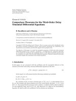
Applying MATLAB, we can draw the graph of fγ with α 0.3, λ 0.5 and verify that
the maximum value of fγ is reached for γ 1.24. On the other hand, the middle γ 1.20.
Therefore, Theorems 2.6 and 2.10 imply that if α 0.3, λ 0.5, and
a>1.1726, then
2.13
has the property
P
0
,
a>41.3856, then
2.13
is oscillatory.
2.27
On the other hand, if we apply the middle γ, we get a bit weaker result for oscillation of
2.13, namely, a>43.1905.
Advances in Difference Equations 9
Remark 2.14. The oscillation of E is a new phenomena in the oscillation theory. The previous
results 3, 5, 13 do not help to study this case, because t hey are based on transferring the
properties of the ordinary equation E
1
to the delay equation E, and since E
1
is not
oscillatory, we cannot deduce oscillation of E from that of E
1
.
Our comparison method is based on the canonical representation E
C
of E.
Although the condition 2.3 of Lemma 2.2 guarantees the existence of the wanted solution
vt of V so that canonical representation E
C
is possible, a natural question arises; what to
do if we are not able to find vt because it is needed in the crucial E
2
and E
3
? In the next
considerations, we crack this problem. Employing the additional condition, we revise both
E
2
and E
3
into the form that instead of vt requires its asymptotic representation which
essentially simplifies our calculations.
We say that v
∗
t is an asymptotic representation of vt if lim
t →∞
vt/v
∗
t 1. We
denote this fact by vt ∼ v
∗
t.
The following result is recalled from 2.
Theorem 2.15. If
∞
sp
s
ds<∞,
2.28
then V has a solution vt with the property vt ∼ 1.
Combining Theorem 2.15 together with Corollaries 2.7 and 2.11, we get new oscillatory
criterion for E.
Theorem 2.16. Assume that 2.28 holds and
lim inf
t →∞
t
τ
t
g
u
τ
u
− t
1
2
2
du>
1
e
, C
∗
1
then E has the property (P
0
).
If, moreover, τ
t > 0 and there exists a function ξt ∈ C
1
t
0
, ∞ such that 2.17 holds
and
lim inf
t →∞
t
η
t
ξu
u
ξs
s
g
x
dx ds du>
1
e
, C
∗
2
then E is oscillatory.
Proof. It follows from Theorem 2.15 that for any C ∈ 0, 1, we have
C<v
t
<
1
C
,
2.29
10 Advances in Difference Equations
1 1.05 1.1 1.15 1.2 1.25 1.3 1.35 1.4 1.45
0
0.002
0.004
0.006
0.008
0.01
0.012
0.014
0.016
0.018
0.02
γ
Max[α = 0.3,λ= 0.5]=0.019645 at
γ = 1.24, middle γ = 1.2071
Figure 1
eventually. Moreover, C
∗
1
implies that there exists C ∈ 0, 1 such that
1
e
< lim inf
t →∞
C
4
t
τt
g
u
τu − t
1
2
2
du
lim inf
t →∞
t
τ
t
Cg
u
τu
t
1
C
s
t
1
1
C
−2
dx ds du
≤ lim inf
t →∞
t
τt
v
u
g
u
τu
t
1
v
s
s
t
1
v
−2
x
dx ds du,
2.30
where we have used 2.29.WeseethatC
1
holds and Corollary 2.7 guarantees the property
P
0
of E.
The proof of the second part runs similarly, and so it can be omitted.
Example 2.17. Consider the third-order trinomial equation of the form
y
t
α
1 − α
t
3
y
t
a
t
3
y
λt
0,
2.31
with 0 <λ<1, 0 <α<1/2, and a>0. It is easy to see that 2.28 holds. Now, C
∗
1
reduces to
aλ
2
2
ln
1
λ
>
1
e
,
2.32
which insures the property P
0
of 2.23.
Advances in Difference Equations 11
On the other hand, setting ξtγt, where 1 <γ<1/
√
λ, the condition C
∗
2
takes the
form
a
2
1 −
1
γ
2
1 −
1
γ
ln
1
λγ
2
>
1
e
.
2.33
If we put γ 1
√
λ/2
√
λ, which is the middle point of the prescribed interval, 2.33 rises
to
a
2
⎛
⎜
⎝
1 −
4λ
1
√
λ
2
⎞
⎟
⎠
1 −
2
√
λ
1
√
λ
ln
⎛
⎜
⎝
4
1
√
λ
2
⎞
⎟
⎠
>
1
e
,
2.34
that in view of Theorem 2.16 yields the oscillation of 2.31.
3. Summary
In this paper, we have presented a new comparison principle for studying the oscillatory and
asymptotic behavior of the third-order delay trinomial equation E. Our method essentially
makes use of its binomial representation E
C
, which is based on the existence of the suitable
positive solution of the corresponding second-order equation V , so that we can deduce
property P
0
or even oscillation of E from the oscillation of a couple of the first-order delay
equations E
2
and E
3
. Moreover, in a partial case, we can examine the studied properties
of E without finding a positive solution of V . Obtained comparison theorems are easily
applicable.
Acknowledgment
This research was supported by S.G.A. KEGA no. 019-025TUKE-4/2010.
References
1 B. Bacul
´
ıkov
´
aandJ.D
ˇ
zurina, “Oscillation of third-order neutral differential equations,” Mathematical
and Computer Modelling, vol. 52, no. 1-2, pp. 215–226, 2010.
2 R. Bellman, Stability Theory of Differential Equations, McGraw-Hill, New York, NY, USA, 1953.
3 J. D
ˇ
zurina, “Asymptotic properties of the third order delay differential equations,” Nonlinear Analysis:
Theory, Methods & Applications, vol. 26, no. 1, pp. 33–39, 1996.
4 J. D
ˇ
zurina, “Comparison theorems for nonlinear ODEs,” Mathematica Slovaca, vol. 42, no. 3, pp. 299–
315, 1992.
5 J. D
ˇ
zurina and R. Kotorov
´
a, “Properties of the third order trinomial differential equations with delay
argument,” Nonlinear Analysis: Theory, Methods & Applications, vol. 71, no. 5-6, pp. 1995–2002, 2009.
6 L. Erbe, “Existence of oscillatory solutions and asymptotic behavior for a class of third order linear
differential equations,” Pacific Journal of Mathematics, vol. 64, no. 2, pp. 369–385, 1976.
7 P. Hartman, Ordinary Differential Equations, John Wiley & Sons, New York, NY, USA, 1964.
8 G. D. Jones, “An asymptotic property of solutions of y
pxy
qxy 0,” Pacific Journal of
Mathematics, vol. 47, pp. 135–138, 1973.
9 G. S. Ladde, V. Lakshmikantham, and B. G. Zhang, Oscillation Theory of Differential Equations with
Deviating Arguments, vol. 110 of Monographs and Textbooks in Pure and Applied Mathematics, Marcel
Dekker, New York, NY, USA, 1987.
12 Advances in Difference Equations
10 I. T. Kiguradze and T. A. Chanturia, Asymptotic Properties of Solutions of Nonautonomous Ordinary
Differential Equations, vol. 89 of Mathematics and Its Applications, Kluwer Academic Publishers,
Dordrecht, The Netherlands, 1993.
11 T. Kusano and M. Naito, “Comparison theorems for functional-differential equations with deviating
arguments,” Journal of the Mathematical Society of Japan, vol. 33, no. 3, pp. 509–532, 1981.
12 A. C. Lazer, “The behavior of solutions of the differential equation x
tPtx
tqtxt0,”
Pacific Journal of Mathematics, vol. 17, pp. 435–466, 1966.
13 N. Parhi and S. Padhi, “On asymptotic behavior of delay-differential equations of third order,”
Nonlinear Analysis: Theory, Methods & Applications, vol. 34, no. 3, pp. 391–403, 1998.
14 N. Parhi and S. Padhi, “Asymptotic behaviour of solutions of third order delay-differential
equations,” Indian Journal of Pure and Applied Mathematics, vol. 33, no. 10, pp. 1609–1620, 2002.
15 Ch. G. Philos, “On the existence of nonoscillatory solutions tending to zero at ∞ for differential
equations with positive delays,” Archiv der Mathematik, vol. 36, no. 2, pp. 168–178, 1981.
16 M. Hasanbulli and Y. V. Rogovchenko, “Oscillation criteria for second order nonlinear neutral
differential equations,” Applied Mathematics and Computation, vol. 215, no. 12, pp. 4392–4399, 2010.
17 Y. V. Rogovchenko and F. Tuncay, “Oscillation criteria for second-order nonlinear differential
equations with damping,” Nonlinear Analysis: Theory, Methods & Applications, vol. 69, no. 1, pp. 208–
221, 2008.
18 A.
ˇ
Skerl
´
ık, “Integral criteria of oscillation for a third order linear differential equation,” Mathematica
Slovaca, vol. 45, no. 4, pp. 403–412, 1995.
19 A. Tiryaki and M. F. Aktas¸, “Oscillation criteria of a certain class of third order nonlinear delay
differential equations with damping,” Journal of Mathematical Analysis and Applications, vol. 325, no. 1,
pp. 54–68, 2007.
20 Z. Xu, “Oscillation theorems related to averaging technique for second order Emden-Fowler type
neutral differential equations,” The Rocky Mountain Journal of Mathematics, vol. 38, no. 2, pp. 649–667,
2008.