Báo cáo hóa học: " Research Article Design and Implementation of a Generic Energy-Harvesting Framework Applied to the Evaluation of a Large-Scale Electronic Shelf-Labeling Wireless Sensor Network" pdf

Hindawi Publishing Corporation
EURASIP Journal on Wireless Communications and Networking
Volume 2010, Article ID 343690, 12 pages
doi:10.1155/2010/343690
Research Article
Design and Implementation of a Generic Energy -Harvesting
Framework Applied to the Evaluation of a Large-Scale Electronic
Shelf-Labeling Wireless Sensor Network
Pieter De Mil,
1
Bar t Jooris,
1
Lieven Tytgat,
1
Ruben Catteeuw,
1
Ingrid Moerman,
1
Piet Demeester,
1
andAdKamerman
2
1
Department of Information Technology (INTEC), Broadband Communication Networks (IBCN), Ghent University,
G. Crommenlaan 8 (bus 201), 9050 Gent, Belgium
2
GreenPeak Technologies, Vinkenburgstraat 2a, 3512 Utrecht, The Netherlands
Correspondence should be addressed to Pieter De Mil,
Received 16 February 2010; Accepted 24 June 2010
Academic Editor: Jiannong Cao
Copyright © 2010 Pieter De Mil et al. This is an open access article distributed under the Creative Commons Attribution License,

which permits unrestricted use, distribution, and reproduction in any medium, provided the original work is properly cited.
Most wireless sensor networks (WSNs) consist of battery-powered nodes and are limited to hundreds of nodes. Battery replacement
is a ver y costly operation and a key factor in limiting successful large-scale deployments. The recent advances in both energy
harvesters and l ow-power communication systems hold promise for deploying large-scale wireless green-powered sensor networks
(WGSNs). This will enable new applications and will eliminate environmentally unfriendly battery disposal. This paper explores
the use of energy harvesters to scavenge power for nodes in a WSN. The design and implementation of a generic energy-harvesting
framework, suited for a WSN simulator as well as a real-life testbed, are proposed. These frameworks are used to evaluate whether a
carrier sense multiple access with collision avoidance scheme is sufficiently reliable for use in emerging large-scale energy harvesting
electronic shelf label (EHESL) systems (i.e., 12000 labels in a star topology). Both the simulator and testbed experiments yielded
an average success rate up to 92%, with an arr ival rate of 40 transceive cycles per second. We have demonstrated that our generic
energy-harvesting framework is useful for WGSN research because the simulator allowed us to verify the achieved results on the
real-life testbed and vice versa.
1. Introduction
The greatest limits faced by wireless sensor networks (WSNs)
are the lifetime and the scale of the deployed networks.
Currently, most of the WSNs are battery-powered, so the
node’s lifetime is equal to the lifetime of the battery it uses.
The vast majority of the research efforts so far have focused
on the development of energy-efficient MAC (medium access
control) and network protocols to guarantee a lifetime of at
least a couple of years with a single battery pack. Typically,
batteries need to be replaced every 3 to 5 years, depending
on the application the WSN is designed for. Changing
the batteries of hundreds or even thousands of nodes is
cumbersome, costly, and environmentally unfriendly. The
manufacturing, recylcing, and disposal of batteries involves a
heavy carbon footprint. Traditional battery-operated WSNs
will have a tremendous impact on the environment, if large-
scale deployments start to roll out. For this reason, most of
the deployed battery-operated WSNs are (luckily?) limited to

a small number of nodes (64 nodes in [1], 100 nodes in [2]).
The cost of changing a node’s depleted batteries can outweigh
the cost of the node itself. This very high operational cost has
to some extent curtailed the proliferation of WSNs.
Ongoing technical development in the field of energy
harvesters led to new opportunities. energy harvesting (EH)
systems scavenge solar, thermal, or mechanical energy from
the ambient environment and convert it into electrical
energy. At the same time, ultra low-power radios have been
developed and miniaturization of the hardware is still going
on. These three evolutions will enable the revolution towards
long-lived, large-scale sensor networks. These wireless green-
powered sensor networks (WGSNs) will no longer depend
2 EURASIP Journal on Wireless Communications and Networking
on batteries with a finite life span, allowing a wide range of
(novel) large-scale applications.
Research on WGSNs implies a shift in the research efforts:
network lifetime is no longer an issue. Instead we can
start to focus on optimizing the application’s requirements
(reliability, throughput, etc.). Of course, new protocols will
have to account for the unique characteristics of energy-
harvesting power sources.
An implementation on a testbed and a correlated sim-
ulation is needed to evaluate an algorithm, a protocol, or a
system. For our WGSN research, a generic energy-harvesting
framework that is able to simulate and emulate an energy
harvester was necessary. This paper describes the design
of that framework (it is implemented both in the Castalia
simulator and on the iLab.t WiLab testbed). Subsequently,
the framework is used to evaluate the packet success rate

of a large-scale energy harvesting electronic shelf labeling
(EHESL) WGSN.
The novelty of this research is the ability to analyse
and evaluate both novel and well-studied protocols in
combination with emulated energy harvesting power sources
(e.g., energy harversters). Most experimental testbeds and
simulators only offer a fixed power supply or a battery
model. This work will facilitate the experimental research for
heterogeneous WSNs, containing a mix of mains-powered,
battery-powered, and energy harvesting power supplies.
The remainder of this paper is organized as follows. The
use case that inspired this research and the requirements are
described in the following section. Next, we briefly discuss
some of the energy-harvesting aspects that are important
to understand the foundation of our energy harvesting
framework (Section 4). Sections 5 and 6 give an overview of
the framework’s implementation on the testbed and in the
simulator. We then present our experimental setup for the
ESL use case in Section 7 and the performance evaluation
in Section 8. Next, related work is discussed and the final
section concludes this paper.
2. An Inspiring Use Case: Large-Scale Electronic
Shelf Labeling
Retailers use ESL for displaying product pricing on shelves.
Each label has the following components: a power source, a
display, and a communication module. The communication
network (wired or wireless) enables the retailer to handle
price changes automatically. No manual intervention is
needed, everything can be managed from the server.
Most ESL systems use either wired communication

networks or wireless communication with battery-powered
labels. In our research, the communication network is a WSN
and the power source of the labels is an energy harvester.
A typical EHESL system would consist of several thousands
indoor solar cell-powered label nodes. They form a star
topology with a central mains powered controller, which is
connected to a price database.
Each label node initiates one transceive cycle by initiating
a CCA. If the channel is found to be clear, the label sends
a request for update (RFU,20bytes,0.832msintheair)to
the controller at a random time in a periodical time interval
U
I
(e.g., 300 seconds in the real use case). The controller
sends back an update (U, 120 bytes, 4.032 ms in the air)
after a fixed time (i.e., 200 ms). This fixed time gap serves
two purposes. First, this gap between RFU and U is needed
because the controller needs to look up the (new) price
in the database. Second, the label will switch off its radio
chip during this lookup process. This minimizes the average
energy consumption of the label.
We identified four requirements of our EHESL system.
Lifetime of the Network and Low Maintenance Cost. The
expected lifetime of an EHESL system is at least 10 years,
and retailers do not want a high-maintenance cost. If the
presented use case works with solar cells, we wil l meet this
requirement.
Scale. The network size is more than ten thousand nodes.
Find out if CSMA-CA is sufficient for our use case and which
parameters (e.g., backoff windows, clear channel assessment,

retries, etc.) are important and which are not.
Critical Network Operation. Due to the fact that the labels are
powered by a solar cell, a critical network operation occurs
when all labels will start around the same time (e.g., after a
night). In this situation, all labels will request an update and
the level of network activ ity (the load) will be very high. The
system must continue to work in this worst-case situation.
Success Rate of Price Updates. Individual success rates must
be bigger than 75% if 12000 labels are requesting an
individual update once every five minutes.
3. Background
In [3], we found that a CSMA-CA (carrier sense multiple
access with collision avoidance) scheme is theoretically suited
and sufficient to minimize collisions between the subsequent
frames of the different nodes. In 2008, GreenPeak Technolo-
gies has designed a prototype (not published previously) of
an electronic shelf label with segmented display and solar
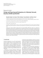
cells. In Figure 1, the block diagram is shown.
The main PCB contains the following blocks:
(i) GreenPeak CM09 radio modules (the new GP500C
was not yet available);
(ii) printed RF antenna;
(iii) power management components;
(iv) connector to display controller board;
(v) RS232 driver;
(vi) debugging interface.
Display controller boards will be different for various
displays. As such it makes the main PCB hardware indepen-
dent of the used display. The display controller board for the
segmented display contains the following blocks:

EURASIP Journal on Wireless Communications and Networking 3
Power
management
Main PCB
CM09
radio
module
RS232
interface
RS232
JTAG
Solar cells
display
controller board
Hirose connectors
Segmented display
Aux pwr
Display
driver
Figure 1: Block diagram of an energy harvesting electronic shelf
label.
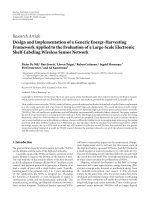
Figure 2: Photo of a fully functional energy harvesting electronic
shelf label. This label has updated the price (70). We also see the
two solar cells on this prototype.
(i) display driver: DA8523 from dialog semiconductor;
(ii) interface connector to the main PCB;
(iii) interface connectors to the 192 segment display: 4
hirose connectors;
(iv) connectors for 2 solar cells, one connector for each
solar cell.

The display used in this prototype is a special designed
192 segment display from E-Ink.
This prototype, see Figure 2,hasproventobefully
functional each and every day, in a small-scale setup, for over
one year.
We wanted to provide empirical e vidence that the EHESL
protocol can work in a large-scale setup. First, we had to
extend the functionality of our testbed and the simulator
with our energy harvesting framework.
4. Energy-Harvesting Aspects
Energy harvesting is the process by which energy from
the physical environment is captured and converted into
usable electrical energy. Before we started to build our
energy-harvester framework, we have identified the typical
components of the real energy harvesters.
An energy-harvesting system generally requires an energy
source (see Section 4.1) and three other key electronic
components, including:
Table 1: Power densities of typical energy harvesters.
Energy source Characteristics Efficiency Power density
Light
Outdoor
10–25%
100 mW/cm
2
Indoor 100 μW/cm
2
Thermal
Human 0.1% 60 μW/cm
2

Industrial 3% 10 mW/cm
2
Vibration
Hz-Human
25–50%
4 μW/cm
2
kHz-Machines 800 μW/cm
2
Radio GSM 900 MHz
50%
0.1 μW/cm
2
frequency WiFi 2.4 GHz 0.001 μW/cm
2
(i) an energy conversion device (see Section 4.2);
(ii) an energy harvesting module that captures, stores,
and manages power for the device (see Section 4.3);
and
(iii) an end application such as the previously presented
ESL use case.
Based on this insight, we will present the foundation of
our energy harvesting framework.
4.1. Overview of Energy Sources. This section highlights some
common sources of energy harvesting [4]:
(i) mechanical energy: from sources such as vibration,
mechanical stress, and st rain;
(ii) thermal energy: waste energy from furnaces, heaters,
and friction sources;
(iii) light energy: captured from sunlight or room light via

photo s ensors, or solar panels;
(iv) natural energy: from the environment such as wind,
water flow, and solar;
(v) human body: a combination of mechanical and ther-
mal energy naturally generated from bioorganisms or
through actions such as walking and sitting.
These energy sources are virtually unlimited and essen-
tially free, if they can be captured at or near the system
location. They behave differently from energy reservoirs such
as batteries. Where the latter can be characterized by their
energy density, the former tend to provide highly fluctuating
amounts of energy and therefore their primary metric for
comparison is power density. Tab le 1 shows some of the
harvesting methods with their power-generation capability
and is a summary of numbers found in recent literature [5].
In [6], the authors have surveyed energy-harvesting sources
for embedded systems.
4.2. Energy Conversion Device. Although some energy har-
vesters provide a stable DC output, the power output
of most energy harvesters is AC or unstable DC. Since
only a stabilized DC voltage is able to power our sensor
nodes, an AC-DC or a DC-DC convertor is necessary to
provide a constant supply voltage to the sensor node. We
assume that these conversion devices are part of the energy
4 EURASIP Journal on Wireless Communications and Networking
Energy profile EH
Application profile
Average energy generation
Average energy consumption
t

E
Figure 3: Energy profile of an energy harvester (EH) and its average
energy generation versus an application profile and its average
energy consumption. The average energy consumed must be lower
than the average energy harvested.
harvester itself, whose output is as a consequence a DC
current I
DC
. The energy-harvesting circuits in [7] show that
this assumption is realistic. T hese circuits also consume
power, so this has to be taken into account during the
experiments.
4.3. Power Storage and Management. Ambient energy
sources are typically low grade and their power output
is highly nonlinear in nature depending upon a variety
of factors. Hence, energy harvesters provide low, variable,
and sometimes unpredictable levels of power. EH energy
generation (i.e., EH energy profile) seldom matches the
energy required by the application or system (application
profile). Figure 3 illustrates this behavior. The application
profile A of a typical monitoring application is relatively flat,
except for periodical spikes (when the radio is turned on).
TheenergyprofileBhasatotallydifferent shape: one day—
night cycle is shown. An additional storage element makes
it possible for B to power A. This intermediate rechargeable
battery or capacitor is needed to catch temporal fluctuations
on or discrepancies between both the application’s and
energy harvester’s energy profile. The storage element is
charged with the DC current I
DC

from the energy harvester.
Once the energy is stored, a minimal condition for an end
application to work is that the average energy consumed is
lower than the average energy harvested.
4.4. Energy-Harvesting Framework. All the elements needed
to construct a generic EH Framework (EHF) are now present:
a variable current provided by the emulated energy harvester
I
DC
(a) to charge an intermediate storage element (b), and an
energy consuming application (c). The framework’s task is
to regulate a realistic balance between these elements. This
is possible by virtualizing (b) and adjusting the (virtual)
voltage potential over this element according to (a) and
(c). This wil l allow us to set a real-time configured voltage
instead of always using a fixed voltage (e.g., 3.0 V). An
ideal (super)capacitor (most suited here due to higher
charge/discharge efficiency) is characterized by (1). C is the
capacitance of the capacitor
v
(
t
)
=
q
(
t
)
C
.

(1)
The current i(t) equals the rate of change of the charge
with respect to t ime
i
(
t
)
=
dq
(
t
)
dt
.
(2)
Physical charges cannot pass through the dielectric layer
of a capacitor, but rather build up in equal and opposite
quantities on the electrodes; As each electron accumulates
on the negative plate, one leaves the positive plate. Thus the
accumulated charge on the electrodes is equal to the integral
of the current, as well as being proportional to the voltage.
Combining (1)and(2) gives us the integral form of the
capacitor equation
v
(
t
)
=
1
C


t
t
0
i
(
τ
)
dτ + v
(
t
0
)
,
(3)
v(t
0
) represents the initial voltage. i(τ) is the difference
between the harvested current and the consumed current.
This equation will be used to keep a record of the available
energy. Note that for rechargeable batteries, another voltage
law is needed, but the general principles remain the same.
We can also use this framework to emulate nonrechargeable
batteries, so we have the foundation for a generic tool that
can emulate energy harvesters and (rechargeable) batteries.
5. Energy Harvesting Framework at Testbed
As already stated in the introduction, real-life testbeds and
simulation platforms are indispensable development tools
for our research. In 2008, IBBT launched a technology center,
called iLab.t. One part of it is the iLab.t WiLab testbed [8].

This WSN testbed consists out of 200 nodes; spread over
three floors of a 12
× 80 m
2
office building. The architecture
of the testbed, as shown in Figure 4, is based on the widely
used MoteLab testbed concept from Harvard University [9].
The motes used are TMote Sky motes. The intermediate
nodes (iNodes) are mini-PCs equipped with ethernet, USB,
serial, VGA, audio, and two 802.11bg wireless network
interfaces. All the iNodes are connected to the management
backbone. Finally, the environment emulator (EE) sits in
between the iNode and the TMote Sky sensor node (
=device
under test (DUT)). Both the iNode and the EE make this
testbed unique and very flexible.
An EE (Figure 5) can emulate scenarios (e.g., battery
depletion, energy harvesting power sources, node failure,
sensor events, actuator events, etc.) in a real-life office
environment without the need for real hardware (batteries,
harvesters, temperature sensors, etc.). We will only discuss
the EE, because this is the hardware/softwarel tool that
enables energy harvesting emulation.
EURASIP Journal on Wireless Communications and Networking 5
Admin interface (new firmware, logging, )
Control interface (emulation of the sensors, )
Central
managment
Ethernet connection (PoE)
···

Switch
iNode
DUT
iNodeiNode
EE
EE EE
DUT
DUT
Figure 4: iLab.t WiLab testbed architecture. The central man-
agement server has an ethernet connection with all the iNodes.
These iNodes provide an admin interface to the environment
emulator (EE), which provides both an admin interface and a
control interface to the device under test (DUT).
iNode
Ethernet + power
Environment
Emulator
DUT
Battery emulator +
real-time power measurements
Audio
USB
Fixed interface:
RS232, USB, etc.
Power
Current
PWR
Serial
I/O
Audio

DAC/ADC
GPIO
Audio
Sensor/actuator emulation
Figure 5: Features of the environment emulator. We have used the
battery emulator and the real-time power measurements for our
energy harvesting emulation.
5.1. Environment Emulator: Hardware. For the design of the
iLab.t WiLab testbed, we created a new board, which is
basicly a stripped version of the TMote Sky and we called it
the environment emulator. By default, the DUT is powered
via USB. If we want to use an alternative power source, the
EE can tear down this USB connection, and powers the DUT
via the expansion connector. Both dedicated hardware and
software were needed to achieve this desired feature.
The general principles of the energy-harvesting emulator
part of the EE are depicted in Figure 6. At the left, we can
see the USB power supply of the board. In the middle, we
measure the current consumed by the DUT. This is used in
a feedback loop, in order to configure the output voltage
for the battery interface of the DUT. The energy harvester
and the storage element (e.g., ultracapacitor) are virtual, and
implemented in software. The voltage drop accros this virtual
capacitor is calculated as described in the next subsection.
For example, our DUT will power up if the voltage is higher
than 1.5 V (1.8 V according to the datasheet of the MSP430).
A
V
A
V

Configurable
output
voltage
Feedback
USB
DUT
Figure 6: General principles of the energy-harvesting emulator. We
measure the current consumed by the DUT, and we set the output
voltage. The characteristics of the energy harvester and the storage
element are implemented in software.
Figure 7 is the schematic that is part of the EE. On
the EE we connected VDD (voltage drain drain) to the
USB power of the board. The ADC (analog-to-digital
converter) and DAC (digital-to-analog converter) lines are
connected to DAC1 and ADC4 of the EE’s MSP430. Next,
the DUT
BATTER Y INTERFACE lines are interfaced to the
battery interface of the DUT (e.g., TMote Sky). Implement-
ing just the schematics as it is and connect it to an existing
TMote Sky or TelosB gives the same functionality (we have
also added other features, like setting/getting GPIO pins of
the DUT, and audio).
The main component in the schematic is U1 which is
a rail-to-rail, high-output current amplifier. U1a is used to
implement a voltage follower and maps the 2.5 V coming
from the DAC (maximum output of DAC1 of the MSP430)
to 3.5 V (the maximum supply voltage of the DUT). Standard
opamp schematics are not able to dr ive high capacitive loads.
C1 and R10 were added in the second version of the EE
and are used as inner and outer loop compensations for a

better response when driving high capacitive loads. 10 uF is a
typical input capacitor of a sensornode and is much higher
than what an opamp (typical 200 pF) can drive without
compensations. U1b is used to implement a differential
amplifier and maps a current of 70 mA through R4 and R5 to
2.5 V on the input of the ADC (the maximum input voltage
of ADC4 of the MSP430).
5.2. Environment Emulator: Software. We already know that
the capacitance (stated in terms of the amount of charge (Q)
stored at a given voltage drop (across the capacitor)) of a
capacitor is given by (1). (Note that: the SI unit of capacitance
is the farad; 1 farad
= 1 coulomb per volt; typical capacitances
are measured in microfarads or picofarads)
5.2.1. The Virtual Capacitor. To implement the law of
Coulomb,aTinyOSapplicationwasdevelopedwherewe
implemented an event ConfigStream with these par ameters:
(i) value
0: start value which is the DAC value at t0. The
value is in the range of [0, 4095]. 4095 maps on 3.48 V.
6 EURASIP Journal on Wireless Communications and Networking
ADC
GND
DAC
R1
R2
R3
R4 R5
R6
R7

R8
R9
R10
C1
C2
1
2
3
4
5
6
7
8
+
−
100 k
120 k
47 k
10
10
24
18 k
90 k9
100 nF
1nF
AD8397ARDZ
U1A
AD8397ARDZ
U1B
GND GND

GNDGNDGND
+
−
90 k9
18 k
VDD
DUT
BATTERY INTERFACE
Figure 7: Electronic circuit schematic of the energy-harvesting emulator.
(ii) harvestMultiplier: this defines the size of the virtual
capacitor, for a given “interSampleDelay” of the
current measurements, and
(iii) harvester: The unit of harvester is 70/4095 mA.
When this ConfigStream event is executed, a continous
sampler will start on ADC4 with an “interSampleDelay” Δt
of 250 μs (4 kHz sampling rate). On every sampler buffer
done event, the next DacValue will be calculated as follows
(sampler buffer size is 50 samples, so we have a reaction time
of 12.5 ms (80 Hz))
DacValue
(
t +1
)
= DacValue
(
t
)
+

50

i=0
harvester − sample Buffer
(
t
)
[
i
]
harvestMultiplier
.
(4)
So, the new DacValue is the sum of the old DacValue
and the delta that is determined by the sum of the
harvested current (greater than or equal to zero) and the
consumed current (smaller or equal to zero), scaled w ith the
harvestMultiplier.
5.2.2. How to Determine the Equivalent Capacitance of the
Virtual Capacitor? We will show how we determine the
size of the equivalent capacitance of the “harvestMultiplier”
(given an “interSampleDelay”). We start from(5)
ΔQ
= C × ΔV = ΔI × Δt,
(5)
ΔQ is the difference in charge (in coulomb); C is the
capacitance of the capacitor (in farad); ΔV is the electrical
potential difference across the virtual capacitor (in Volt); and
ΔI is the difference between the har vested current (virtual,
determined by “harvester”) and the consumed current (real
current measurement) in ampere over the sample period Δt.
We can rew rite (5):

ΔI
ΔV
=
C
Δt
.
(6)
The embedded software on the EE calculates (7):
ΔV

=
ΔI

harvestMultiplier
,
(7)
ΔV

is the electrical potential difference across the
virtual capacitor (range [0, 4095] DAC); ΔI

is the difference
between the harvested current and the consumed current
(range [0, 4095] ADC)
ΔV
= ΔV

×
3.48
4095

,
ΔI
= ΔI

×
0.070
4095
.
(8)
Combining (8), it follows that
49.71
×
ΔI
ΔV
=
ΔI

ΔV

.
(9)
Combining (6), (7), and (9), it follows that
49.71
×
C
Δt
= harvestMultiplier.
(10)
We round up this factor to 50 (increase with 0.58%)
C

= harvestMultiplier ×
Δt
50
.
(11)
With an “interSampleDelay” Δt of 250 μs, and a “harvest-
Multiplier” of 1; the unit of the equivalent capacitance of the
virtual capacitor is 5 μF(11) (200 k is 1F).
EURASIP Journal on Wireless Communications and Networking 7
0
5
10
15
20
25
30
35
40
0
76
152
228
304
380
456
532
608
684
760
836

912
988
1064
1140
1216
1292
1368
1444
Samples (25 ms)
Voltage and current consumption on node 8 (battery emulation)
Voltage (dV)
Current (mA)
Figure 8: Battery emulation on node 8: 3.49 V and 2000 mAh
capacity. T he application sends one packet every 7 second (ran-
dom). The available energy decreases very slowly.
5.3. Validation. We have tested our implementation of
the energy-harvesting framework on the testbed with two
examples: battery emulation and solar cell emulation. The
emulation of the power source is done on the EE, which
powers the DUT. The parameters needed by our framework
are managed via a web-based interface, which configures
each EE. This means that the generic energy harvesting
framework (on the EE) is independent from the application
on the DUT. This way, the application does not need
to implement an API, so any existing application can be
evaluated. We have evaluated a retail application but it is
possible and desirable to evaluate other application domains
like agricultural machinery, building or home automation,
structural health monitoring, and so forth.
5.3.1. Battery Emulation. For a battery emulation of 3.49 V

and 2000 mAh, we could define a full battery with initial
voltageof3.49Vandaharversterwhichisequaltozeroand
a capacitor of 2063 F (C
∗
3.49 V = 2A
∗
3600 s) or the virtual
capacitor equal to 412600 k (2063
∗
200 k). In Figure 8, the
blue line is the voltage, starting at 34.9 dV and it will decrease
very slowly. This demo application is sending a packet once
every second. In red, we can see the average current measured
by the EE.
5.3.2. Solar Cell Emulation. For a small energy harvester
emulation, we could define a capacitor with initial voltage
of 0 V and a harverster which is equal to 0.855 mA (50) and
a capacitor of 875 μF. On the DUT, the first thing to do is
to check if there is enough energy and if the radio can be
enabled. Failing to do this would put the DUT in an endless
reboot sequence. In Figure 9, the blue line is the voltage,
starting at 0 dV and it will increase until 35 dV (3.5 V). The
application tries to send a packet, once every ten seconds
(randomly chosen). Next, it will listen three times. We can
see this in red. The feedback mechanism works: more current
is consumed than harvested and the voltage drops.
0
5
10
15

20
25
30
35
40
0 100
200
300
400
Samples (25 ms)
Voltage and current consumption on node 8 (energy harvester emulation)
Voltage (dV)
Current (mA)
Transmit
Receive
Figure 9: Energy-har vester emulation. Initially, there is no available
energy. The application transmits one packet and listens three times.
We see that the voltage drops during the radio activ ities and that it
increases when more energy is harvested than is consumed (until
the capacitor’s maximum is reached).
6. Energy Harvesting Framework at Simulator
We also wanted a high level of flexibility in the simulation
environment. Castalia [10] was created out of the need to
have a simulator designed for WSN research. It has advanced
and accurate radio and wireless channel models. Castalia is
built on OMNeT++, a framework which provides the basic
tools to write simulators. In Castalia, nodes are OMNet++
modules. This makes it easy to add our energy harvesting
framework. We will briefly discuss the software extension,
without going into details.

6.1. Software. Castalia’s resource-manager module
(Figure 10) manages the avalaible resources (consumed
energy, CPU-time, etc.) of a simulated node. It is extended
with our energy harvesting model. By providing harvesting
functionality and an interface to the application ( power
node up, and down), a first version was implemented. This
had some shortcomings; like the fact that the radio module
was solely responsible for executing the harvesting function
and determining the amount of harvested energy. A second
problem was the unrealistic effect of the system: the adjusted
model assumes that the power source is a rechargeable
battery that provides always a fixed current/voltage, charges
and discharges linearly, and so forth. A realistic system will
not work if the supplied voltage is too low and will restart
if the supplied voltage is above a threshold. Therefore, we
have designed a second version, which is a generic solution.
We have two elements: a configuration file resourceMgr-
Energy-Harvester.ini and a function evaluateEnergy (double
startTime, double amount) (the argument “amount” is the
consumed charge).
8 EURASIP Journal on Wireless Communications and Networking
To/from physical process
Sensing device manager
Radio
MAC
Network (routing)
Application
Resource manager
Battery
CPU state

Time
Memory
Energy harvesting
framework
Communications
composite module
To/from wireless channel
Figure 10: Internal structure of a node composite module in the
Castalia simulator. We have extended the resource manager with our
energy harvesting framework.
In the configuration file, we can configure the following
parameters:
(i) SN.nodenodeID[nodeID].nodeResourceMgr.harvest
Level-i: i goes from 1 to 20. These values (HL
i
)
determine the levels of harvested current;
(ii) SN.node[nodeID].nodeResourceMgr.harvestInterval
Time: determines when the harvestLevel must switch
to the new level;
(iii) SN.node[nodeID].nodeResourceMgr.capacitor: sets
the value of the virtual capacitor ;
(iv) SN.node[nodeID].nodeResourceMgr.activateHarv-
ester: activate or deactivate the simulated harvester;
(v) SN.node[nodeID].nodeResourceMgr.initialEnergy:
sets the initial voltage accros the virtual capacitor.
The function evaluateEnergy (in the radio module)
contains the logic of our energy harvester framework. If the
voltage across the virtual capacitor goes under a threshold, a
“resource mgr out of energy” message is sent to the modules.

Each module that receives this message will stop handling
the messages (except for the “node start up” message). Now,
the resource manager has to call the evaluateEnergy function
periodically (because the radio module is down). If the
voltage increases again, and a threshold is passed; a “Node
start up” message is sent to the modules. In Figure 11 we see
that the energy is evaluated during each radio transition, over
aperiodD(t
i+1
− t
i
).
HarvestLevel
i+2
HL
c
t
0
t
1
D
δ
a
δ
b
I
D = t
1
− t
0

= δ
a
+2∗ I + δ
b
HL
i+1
HL
i
Figure 11: The energy harvesting concept in the Castalia simulator.
The energy is evaluated during each radio transition, over a period
D taking into account the configured harvestLevels (HL) and the
consumed energy (which is known for each radio state).
Now we have the tools, we can provide experimental
results that prove that an ESL system can work with energy
harvesters (EHESL).
7. Experimental Setup
In our experiments, B-MAC [11] is used. This MAC protocol
uses clear channel assessments (CCA) and packet backoffs
for channel arbitration We have disabled B-MAC’s link layer
acknowledgments and low-power listening functionality
because we only want to use CSMA-CA.
An important limit of our ESL system is the number of
transceive cycles per second the controller can process. We
allow one controller in our network, so this limit determines
the number of labels we can allow in an update interval U
I
.
Suppose we want 16000 labels and U
I
is five minutes. This is

anarrivalrateof53.3RFUspersecond.Theexperimentally
determined maximum arrival rate between two testbed
nodes is 49.3 RFUs per second. Of course, another hardware
platform and/or software stack will have another limit. We
have dimensioned our experiments so that the maximum
average a rrival rate is 40 RFUs per second. This corresponds
with 12000 labels (U
I
= 300 seconds). Clearly, there is
atradeoff between the number of labels and the update
interval.
Since we do not have 12001 testbed nodes, we had to
scale the frequency of the transceive cycles per label in such a
way that the workload λ (RFU arrivals per second) for the
controller is equivalent with a situation with more nodes
(i.e., 12000 labels) transceiving at a lower frequency (i.e.,
once every 300 seconds). We have used 40+1 nodes, thus the
U
I
is one second. One label in our testnetwork corresponds
with 300 emulated labels. We have verified in the Castalia
simulator that this approach is justified.
To make realistic backtracking of the experimentally
achieved results possible, we have added the positions of
the nodes and connectiv ity information (we measured both
received signal strength indication and packet-reception ra-
tio values on our testbed) to the Castalia simulator. The
positions were added in “node
locations.ini” (SN.deploy-
mentType

= 3), and the connectivity information in “rxSig-
nal
ConnectivityMap” and “PRR ConnectivityMap” in the
.ini file of the wireless channel module.
EURASIP Journal on Wireless Communications and Networking 9
Table 2: Parameters.
Parameter Label Controller
Link-layer acknowledgments? No No
Retries? No No
IBW (ms) 0 0
CBW (ms) 8 0
First, we have tested our system without energy harvest-
ing and always-on labels (ESL). Each ESL label sends (or tries
to send) 200 RFUs to the controller, during 200 seconds.
The number of succesfully received updates determines the
success rate of that label. As already stated, we did not use
link-layer acknowledgments or retries. The initial backoff
window (IBW) is zero for both controller and labels. The
congestion backoff window (CBW) is zero for the controller,
and eight ms for the labels. This is summarized in Tabl e 2.
Next, we h ave applied our energy harvesting framework, and
we have tested our system again (EHESL).
8. Analysis of Experiments
The average success rate (S
avg
) is 91% on the tesbed and
91.5% in Castalia. Although the average success rate is stable,
individual success rates (S
ind
) are not: temporal and spatial

fluctuations tend to have a huge impact and can exclude
certain nodes from the network temporarily or permanently.
AveryhighS
avg
is needed to have a working system, but also
individual success rates of all the different ESL labels must
be high enough. The average negative deviation of the S
ind
compared to the S
avg
is 3% (testbed) and 3.5% (simulator);
the maximum negative deviation is 11.5% (testbed) and 12%
(simulator).
The S
ind
varies between 80% and 100%. Figures 12 and
13 show the spatial distribution of the individual success
rate S
ind
of each label on the testbed and in the simulator.
Depending on the success rate, the results were divided in
four categories.
Figure 14 gives an overview of the messages between one
controller and three labels (A, B, and C). It is important
to know when collisions can occur. We have identified four
potential collisions.
(1) Label sending an RFU - label sending an RFU: label A
and label C are hidden nodes. Therefore it is possible
that both RFUs collide at the controller.
(2) Receiving an RFU - sending a scheduled update: If the

controller’s radio is busy receiving an RFU, it cannot
send the scheduled update. This is a problem because
the label will only listen to the medium for a short
time. If the update from the controller cannot be sent
to the label, the label is out of energy due to idle
listening.
(3) Sendingtwoscheduledupdates:This “collision” is
possible because the length of an RFU is six times
smaller than the length of an update. It will be
impossible to send updates to labels that have s ent an
RFU within 3.2 ms after another label’s RFU,because
the controller will be busy sending the update. If we
could schedule all the RFUs, the throughput of the
controller would be 124 RFU/updates in 1 second.
We will see that our experimental setup has a much
lower controller’s throughput (49.2 RFU/updates in
1 second). Since it is impossible to synchronize all
the green-powered labels, it is a good thing that the
controller’s real throughput is limited to 39.7% of the
ideal schedule. This will increase the success rate of
the random RFU/update transceive cycles.
(4) Sending a scheduled update - receiving an RFU: The
controller does not know when RFUs are sent. If
transmission of an update is busy, the controller will
not receive the RFU.
We have also noticed that labels located at the corners
and/or extremes of the floor have lower individual success
rates. Labels in the neighborhood of the controller have the
highest success rate. We have two explanations.
(i) If the distance between label and controller increases,

more packets get lost due to path loss.
(ii) Labels situated at the corners or extremes of the floor
have less connectivity with the other labels in the
network. The hidden node problem occurs when a
label is visible from a controller, but not from other
labels communicating with the controller. This leads
to reduced individual success rates.
Some other conclusions of our experiments are the
following:
(i) Clear channel assessments are very important for
achieving a high success rate in a dense network.
Without CCAs, the S
avg
is 74.5%.
(ii) Backoff window sizes did not have a substantial
impact on the success ra te (explained by the fact that
the labels wake-up randomly already, so there is no
need to add initial backoffs at the MAC layer). The
benefits of using larger contention backoff sizes will
become bigger with a higher network load.
(iii) When transmissions collide a first arriving one will be
received correctly as long as the second arriving one
is received at a sufficiently lower level. This favors the
labels that have a smaller distance to the controller.
9. Related Work
EnergyBucket [12] is a tool for power profiling and
debugging of sensor nodes. It is designed for empirical
measurements of energy consumptions accross 5 decades
of current draw and facilitates easy score-keeping of energy
consumption between different parts of a target application.

This tool can decide when a bucket of 1.22 mJ is used (the
resolution of our tool is 12.81 nJ per 0.25 ms (if we use the
same voltage supply)). The disadvantages are that (1) it is
expensive (TMote Sky + COTS components with a total price
of 150 euro), (2) it is not suited for a whole testbed, and (3)
10 EURASIP Journal on Wireless Communications and Networking
3B45
3B41
3A1
3A31
3A43A73A113A143A183A223A263A28
3A10
3A203A21
3A19
3A15 3A8 3A2
3A16 3A9 3A6 3A3
3A23
3B523B483B363B33
3B53
3B543B51
3B49
3B50
3B463B42
3B43
3B37
3B38
3B34
3B35
3A27
Controller

Third floor of the iLab.t WiLab testbed
Best
Wor st
Success rate
Figure 12: Spatial distribution of the individual success rate on the third floor of the iLab.t WiLab testbed. 4 categories: green = best, yellow,
orange, and red (worst). The blue node is the controller.
3B45
3B41
3A1
3A31
3A43A73A113A143A183A223A263A28
3A10
3A203A21
3A19
3A15 3A8 3A2
3A16 3A9 3A6 3A3
3A23
3B523B483B363B33
3B53
3B543B51
3B49
3B50
3B463B42
3B43
3B37
3B38
3B34
3B35
3A27
Controller

Third floor of the iLab.t WiLab testbed
Best
Wor st
Success rate
Figure 13: Spatial distribution of the individual success rate in the Castalia simulator. 4 categories: green = best, yellow, orange, and red
(least good). The blue nodes are not used.
it delivers a constant volatage of 3.0 V to the target system (it
is not capable to emulate power sources).
PowerBench [13] is a scalable testbed infrastruc ture for
benchmarking power consumption. This 24-node tesbed is
capable of recording the power consumption of all nodes
with a 5 kHz sampling rate and 30 μA resolution. This is
accomplished by means of low-cost interface board, similar
to the one we presented. The disadvantages are that (1) it also
measures the current used by the USB circuit that powers
the DUT, (2) it suffers from instabilities at higer measured
currents (comparible with the first version of the presented
EE, which we solved in the second version), and (3) it delivers
a constant voltage of 3.0 V to the target system (like Energy
Bucket, is not capable to emulate power sources).
Both EnergyBucket and PowerBench share the disad-
vantage that it is not possible to feedback the measured
current to the power supply regulator. This way, both supply
a constant voltage. The EE can power the target system
via its battery interface with a variable voltage supply.
The EE has all the advantages, except for EnergyBucket’s
hardware annotation of program sections (we could add this
functionality because we have extra I/O pins available on the
EE). With the EE, it is also possible to disable the USB circuit,
we have deployed in on 200 nodes, it is less expensive (70

euro), it records the power consumption on all nodes with a
sampling rate of 4 kHz (250 μs), and it can supply the voltage
with a rate of 80 Hz (12.5 ms). Therefore, the EE is beyond
the state-of-the-art, and it is the first tool that enables testbed
experiments of WGSNs. It is also very flexible because each
energy harvester can be emulated.
EHESL is not the only use case using energy harvesting.
Examples of energy harvesting sensor networks include the
following:
(i) WSN-HEAP [14](WSN-poweredsolelybyambi-
ent energy harvesting) uses piezoelectric devices to
transform ambient vibrations into electric energy. It
uses a star topology with multiple sinks. The sinks
are (mains powered) wireless nodes. This solution is
deployed to monitor the health of railroad infrastruc-
ture. The energy harvesting devices uses vibrations
induces by passing trains to gain power. They control
the transmit power of the energy harvesting devices
in order to achieve an optimal node lifetime and
throughput.
(ii) Indoor solar energy harvesting for sensor network
router nodes [15]: this paper describes a solution
for wireless patient health monitoring in hospitals.
The wireless sensing nodes are battery powered and
attached to the patient. The wireless network infras-
tructure nodes use solar cells to transform indoor
light into electrical energy. The y insure connectivity
by using node pairs each with a duty cycle of
50%.
EURASIP Journal on Wireless Communications and Networking 11

Label A
Label B
Label C
Controller
Tx
Tx
Tx
Tx
Rx
Rx
Rx
Rx
RFU
RFU
RFU
200 ms
RFU
RFU
U
200 ms
U
U
U
RFU
RFU
(1)
(2) (3) (4)
cca
cca
cca

cca
cca
Figure 14: Transmit (Tx) and receive (Rx) timeline for one controller and three labels. Labels send a request for update (RFU) to the
controller, the controller replies with an Update (U) after 200 ms. Four potential collisions of messages are identified.
(iii) An environmental energy-harvesting framework for
sensor networks [16] gives a theoretical approach for
using the changes in environmental characteristics to
extend the networks lifetime. They extract more work
out of the same energy environment by adapting the
task distribution among nodes in accordance with
the detailed characteristics of environmental energy
availability. This is a distributed framework where
sensor nodes adaptively learn how much energy they
can extract from the environment and which tasks
they can perform with the given energy.
(iv) Energy harvesting in a mobile sensor network [17]
uses a different approach compared to the previously
described solutions. They exploit the use of mobile
devices to supply energy across the network. These
mobile devices or robots can do this while perfor m-
ing another task. The robots are charged in a docking
station. When the robots are operational they localize
the sensor node with the highest energy requirement
and recharge this sensor node. They do this until their
energy is nearly depleted.
None of these have the same requirements of the presented
EHESL use case. We have focussed on the packet success rate
in a large-scale star topology.
10. Conclusion
This paper presents our energy harvesting framework. We

have described the design of this framework and the
implementation on our testbed and in the Castalia simulator.
Extending the testbed was possible thanks to the earlier
developed hardware platform (the environment emulator)
that is now used to implement the emulation of energy
harvesters (and power sources in general). We have used
two features of the EE. First, the EE can disconnect the USB
power of the device under test (DUT ) and it can power the
DUT via its battery interface with a variable voltage supply.
Second, by measuring the cur rent at a high sample rate and
using this information to control the voltage supply we can
build a controlled loop feedback mechanism. To emulate the
real behavior of an energy harvester, we implemented the law
of Coulomb as a feedback mechanism. Furthermore, we can
determine the exact power consumption as we are at all times
aware of the consumed current by the DUT and the tuned
voltage.
We have successfully applied this energy harvesting
framework to the inspiring ESL use case. The challenge was:
let 12000 nodes request a price update every five minutes and
achieve individual success rates h igher than 75%. We have
showed that the minimum individual success rate was 80%.
Finally, we achieved a very good correlation of simulation
and (scaled) experimental results. This is important because
very large-scale testbed (i.e., more than 10000 nodes) are
too expensive to deploy. The presented framework and
the correlation between the testbed and the simulator will
contribute to the design, implementation, and evaluation of
a broad range of wireless green-powered sensor networks.
References

[1] S. Kim, S. Pakzad, D. Culler et al., “Health monitoring of civil
infrastructures using wireless sensor networks,” in Proceedings
of the 6th International Symposium on Information Processing
in Sensor Networks (IPSN ’07), pp. 254–263, April 2007.
[2] R. N. Murty, G. Mainland, I. Rose et al., “CitySense: an urban-
scale wireless sensor network and testbed,” in Proceedings of the
IEEE International Conference on Technologies for Homeland
Security (HST ’08), pp. 583–588, May 2008.
[3] K. Steenbergen and A. Kamerman, “Scalable wireless sensor
networks based on green energy,” in Wireless Congress: Systems
and Applications, Munchen, Germany, 2008.
[4] />[5] A. Valenzuela, “Batteryless energy har vesting for embedded
designs,” 2009, />[6] S. Chalasani and J. M. Conrad, “A survey of energy harvesting
sources for embedded systems,” in IEEE Southeastcon, pp. 442–
447, Huntsville, Ala, USA, April 2008.
[7] M. J. Guan and W. H. Liao, “Characteristics of energy storage
devices in piezoelectric energy harvesting systems,” Journal of
Intelligent Material Systems and Structures,vol.19,no.6,pp.
671–680, 2008.
[8] L. Tytgat, B. Jooris, P. De Mil et al., “Demo abstract:
WiLab, a real-life wireless sensor testbed with environment
emulation,” in Proceedings of the European Conference on
Wireless Sensor Networks (EWSN ’09), Cork, Ireland, 2009,
/>[9] G. Werner-Allen, P. Swieskowski, and M. Welsh, “MoteLab:
a wireless sensor network testbed,” in Proceedings of the 4th
12 EURASIP Journal on Wireless Communications and Networking
International Symposium on Information Processing in Sensor
Networks (IPSN ’05), pp. 483–488, April 2005.
[10] “Castalia Simulator,” />[11] J. Polastre, J. Hill, and D. Culler, “Versatile low power
media access for wireless sensor networks,” in Proceedings

of the 2nd International Conference on Embedded Networked
Sensor Systems (SenSys ’04), pp. 95–107, New York, NY, USA,
November 2004.
[12] J. Andersen and M . T. Hansen, “Energy Bucket: a tool
for power profiling and debugging of sensor nodes,” in
Proceedings of the 3rd International Conference on Sensor
Technologies and Applications (SENSORCOMM ’09), pp. 132–
138, June 2009.
[13] I. Haratcherev, G. Halkes, T. Parker, O. Visser, and K.
Langendoen, “PowerBench: a scalable testbed infrastructure
for benchmarking power consumption,” in Proceedings of
the International Workshop on Sensor Network Engineering
(IWSNE ’08), 2008.
[14] W. K. G. Seah, A. E. Zhi, and H P. Tan, “Wireless sensor
networks powered by ambient energy harvesting (WSN-
HEAP)—survey and challenges,” in Proceedings of the 1st Inter-
national Conference on Wireless Communication, Vehicular
Technology, Information Theory and Aerospace and Electronic
Systems Technology, Wireless (VITAE ’09), pp. 1–5, May 2009.
[15] A. Hande, T. Polk, W. Walker, and D. Bhatia, “Indoor
solar energy harvesting for sensor network router nodes,”
Microprocessors and Microsystems, vol. 31, no. 6, pp. 420–432,
2007.
[16] A. Kansal and M. B. Srivastava, “An environmental energy
harvesting framework for sensor networks,” in Proceedings of
the International Symposium on Low Power Electronics and
Design, pp. 481–486, Seoul, Korea, August 2003.
[17] M. Rahimi, H. Shah, G. S. Sukhatme, J. Heideman, and D.
Estrin, “Studying the feasibility of energy harvesting in a
mobile sensor network,” in Proceedings of the IEEE Interna-

tional Conference on Robotics and Automation (ICRA ’03),pp.
19–24, Taipei, Taiwan, September 2003.