Báo cáo hóa học: " Research Article Adaptive Modulation with Smoothed Flow Utility" pot
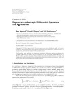
Bạn đang xem bản rút gọn của tài liệu. Xem và tải ngay bản đầy đủ của tài liệu tại đây (984.06 KB, 9 trang )
Hindawi Publishing Corporation
EURASIP Journal on Wireless Communications and Networking
Volume 2010, Article ID 815213, 9 pages
doi:10.1155/2010/815213
Research Article
Adaptive Modulation with Smoothed Flow Utility
Ekine Akuiyibo and Stephen Boyd
Information Systems Laboratory, Department of Electrical Engineering, Stanford University, Stanford, CA 94305, USA
Correspondence should be addressed to Ekine Akuiyibo,
Received 6 May 2010; Accepted 14 September 2010
Academic Editor: Athanasios Vasilakos
Copyright © 2010 E. Akuiyibo and S. Boyd. This is an open access article distributed under the Creative Commons Attribution
License, which permits unrestricted use, distribution, and reproduction in any medium, provided the original work is properly
cited.
We consider the problem of choosing the data flow rate on a wireless link with randomly varying channel gain, to optimally
trade off average transmit power and the average utility of the smoothed data flow rate. The smoothing allows us to model the
demands of an application that can tolerate variations in flow over a certain time interval; we will see that this smoothing leads to
a substantially different optimal data flow rate policy than without smoothing. We pose the problem as a convex stochastic control
problem. For the case of a single flow, the optimal data flow rate policy can be numerically computed using stochastic dynamic
programming. For the case of multiple flows on a single link, we propose an approximate dynamic programming approach to
obtain suboptimal data flow rate policies. We illustrate, through numerical examples, that these approximate policies can perform
very well.
1. Introduction
We consider the flow rate assignment problem on a wireless
link with randomly varying channel gain, to optimally trade
off average transmit power and the average utility of the
smoothed flow data rate. We pose the multiperiod problem
as an infinite-horizon stochastic control problem with linear
dynamics and convex objective. For the case of a single
flow, the optimal policy is easily found using stochastic
dynamic programming (DP) and gridding. For the case of
multiple flows, DP becomes intractable, and we propose
instead an approximate dynamic programming approach
using suboptimal policies developed in the single-flow case.
Simulations show that these suboptimal policies perform
very well.
In the wireless communications literature, varying a
link’s transmit rate (and power) depending on channel
conditions is called adaptive modulation (AM); see, for
example, [1–5].OnedrawbackofAMisthatitisaphysical
layer optimization technique with no knowledge of upper
layer optimization protocols. Maximizing a total utility
function is also very common in various communications
and networking problem formulations, where it is referred
to as network utility maximization (NUM); see, for example,
[6–10]. In the NUM framework, performance of an upper
layer protocol (e.g., TCP) is determined by utility of flow
attributes, for example, utility of link flow rate.
Our setup involves both adaptive modulation and utility
maximization but is nonstandard in several respects. We
consider the utility of the smoothed flows, and we consider
multiple flows over the same wireless link [11].
2. Problem Setup
2.1. Average Smoothed Flow Uti lity. A wireless communi-
cation link supports n data flows in a channel that varies
with time, which we model using discrete-time intervals t
=
0, 1,2, Welet f
t
∈ R
n
+
be the data flow rate vector on the
link, where (f
t
)
j
, j = 1, , n, is the jth flow’s data rate at
time t and R
+
denotes the set of nonnegative numbers. We
let F
t
= 1
T
f
t
denote the total flow rate over all flows, where 1
is the vector with all entries one. The flows, and the total flow
rate, will depend on the random channel gain (through the
flow policy, described below) and so are random variables.
We will work with a smoothed version of the flow rates,
which is meant to capture the tolerance of the applications
using the data flows to time variations in data rate. This
was introduced in [12] using delivery contracts, in which
the utility is a function of the total flow over a given time
interval; here, we use instead a very simple first-order linear
2 EURASIP Journal on Wireless Communications and Networking
smoothing. At each time t, the smoothed data flow rate
vector s
t
∈ R
n
+
is given by
s
t+1
= Θs
t
+
(
I − Θ
)
f
t
, t = 0, 1, ,
(1)
where Θ
= diag(θ), θ
j
∈ [0, 1), j = 1, , n, is the smoothing
parameter for the jth flow, and we take s
0
= 0. Thus, we have
(
s
t
)
j
=
t−1
τ=0
1 − θ
j
θ
t−1−τ
j
f
τ
j
,
(2)
where at time t, each smoothed flow rate (s
t
)j is the
exponentially weighted average of previous flow rates.
The smoothing parameter θ
j
determines the level of
smoothing on flow j. Small smoothing parameter values (θ
j
close to zero) correspond to light smoothing; large values
(θ
j
close to one) correspond to heavy smoothing. (Note
that θ
j
= 0 means that flow j is not smoothed; we have
(s
t+1
)
j
= ( f
t
)
j
.) The level of smoothing can be related to
the time scale over which the smoothing occurs. We define
T
j
= 1/ log(1/θ
j
) to be the smoothing time associated with
flow j. Roughly speaking, the smoothing time is the time
interval over which the effect of a flow on the smoothed
flow decays by a factor 1/e. Light smoothing corresponds to
short smoothing times, while heavy smoothing corresponds
to longer smoothing times.
We associate with each smoothed flow rate (s
t
)
j
a
strictly concave nondecreasing differentiable utility function
U
j
; R
+
→ R, where the utility of (s
t
)
j
is U
j
((s
t
)
j
). The
average utility derived over all flows, over all time, is
U = lim
N →∞
E
1
N
N−1
t=0
U
(
s
t
)
,
(3)
where U(s
t
) = U
1
((s
t
)
1
)+··· + U
n
((s
t
)
n
). Here, the
expectation is over the smoothed flows s
t
,andweare
assuming that the expectations and limit above exist.
While most of our results will hold for more general
utilities, we will focus on the family of power utility
functions, defined for x
≥ 0as
U
(
x
)
= βx
α
,
(4)
parameterized by α
∈ (0,1) and β>0. The parameter α
sets the curvature (or risk aversion), while β sets the overall
weight of the utility. (For small values of α, U approaches a
log utility.)
Before proceeding, we make some general comments on
our use of smoothed flows. The smoothing can be considered
as a type of time averaging; then we apply a concave utility
function; finally, we average this utility. The time averaging
and utility function operations do not commute, except
in the case when the utility is linear (or affine). Jensen’s
inequality tells us that average smoothed utility is greater
than or equal to the average utility applied directly to the flow
rates, that is,
U
(
s
t
)
j
≥
1
t
t−1
τ=0
1 − θ
j
θ
t−1−τ
j
U
f
τ
j
.
(5)
So the time smoothing step does affect our average utility; we
will see later that it has a dramatic effect on the optimal flow
policy.
2.2. Average Power. We model the wireless channel with
time-varying positive gain parameters g
t
, t = 0, 1, ,which
we assume are independent identically distributed (IID),
with known distribution. At each time t, the gain parameter
affects the power P
t
required to support the total data flow
rate F
t
. The power P
t
is given by
P
t
= φ
F
t
, g
t
,
(6)
where φ : R
+
× R
++
→ R
+
is increasing and strictly convex in
F
t
for each value of g
t
(R
++
is the set of positive numbers).
While our results will hold for the more general case,
we will focus on the more specific power function described
here. We suppose that the signal-to-interference-and-noise
ratio(SINR)ofthechannelisgivenbyg
t
P
t
.(Hereg
t
includes the effect of time-varying channel gain, noise, and
interference.) The channel capacity is then μlog(1 + g
t
P
t
),
where μ is a constant; this must equal at least the total flow
rate F
t
,soweobtain
P
t
= φ
F
t
, g
t
=
e
F
t
/μ
− 1
g
t
.
(7)
The total average power is
P = lim
N →∞
E
1
N
N−1
t=0
P
t
,
(8)
where, again, we are assuming that the expectations and limit
exist.
2.3. Flow Rate Control Problem. Theoverallobjectiveisto
maximize a weighted difference between average utility and
average power,
J
= U − λP,
(9)
where λ
∈ R
++
is used to trade off average utility and power.
We require that the flow policy is causal; that is, when
f
t
is chosen, we know the previous and current values of
the flows, smoothed flows, and channel gains. Standard
arguments in stochastic control (see, e.g., [13–17]) can be
used to conclude that, without loss of generality, we can
assume that the flow control policy has the form
f
t
= ϕ
s
t
, g
t
,
(10)
where ϕ : R
n
+
×R
++
→ R
n
+
. In other words, the policy depends
only on the current smoothed flows and the current channel
gain value.
The flow rate control problem is to choose the flow rate
policy ϕ to maximize the overall objective in (9). This is
a standard convex stochastic control problem, with linear
dynamics.
2.4. Our Results. We let J
be the optimal overall objective
value and let ϕ
be an optimal policy. We will show that in
the general (multiple-flow) case, the optimal policy includes
a “no-transmit” zone, that is, a region in the (s
t
, g
t
)space
in which the optimal flow rate is zero. Not surprisingly,
EURASIP Journal on Wireless Communications and Networking 3
the optimal flow policy can be roughly described as waiting
until the channel gain is large, or until the smoothed
flow has fallen to a low level, at which point we transmit
(i.e., choose nonzero f
t
). Roughly speaking, the higher the
level of smoothing, the longer we can afford to wait for a
large channel gain before transmitting. The average power
required to support a given utility level decreases, sometimes
dramatically, as the level of smoothing increases.
We show that the optimal policy for the case of a
single flow is readily computed numerically, working from
Bellman’s characterization of the optimal policy, and is not
particularly sensitive to the details of the utility functions,
smoothing levels, or power functions.
For the case of multiple flows, we cannot easily compute
(or even represent) the optimal policy. For this case we
propose an approximate policy, based on approximate
dynamic programming [18, 19]. By computing an upper
bound on J
, by allowing the flow control policy to use
future values of channel gain (i.e., relaxing the causality
requirement [20]), we show in numerical experiments that
such policies are nearly optimal.
3. Optimal Policy Characterization
3.1. No Smoothing. We first consider the special case Θ = 0,
in which there is no smoothing. Then we have s
t
= f
t−1
,so
the average smoothed utility is then the same as the average
utility, that is,
U = lim
N →∞
E
1
N
N−1
t=0
U
f
t
.
(11)
In this case the optimal policy is trivial, since the stochastic
control problem reduces to a simple optimization problem
at each time step. At time t, we simply choose f
t
to maximize
U( f
t
) − λP
t
. Thus, we have
ϕ
s
t
, g
t
=
arg max
f
t
≥0
U
f
t
−
λP
t
,
(12)
which does not depend on s
t
. A simple and effective approach
is to presolve this problem for a suitably large set of values
of the channel gain g
t
and store the resulting tables of
individual flow rates ( f
t
)
i
versus g
t
; online we can interpolate
between points in the table to find the (nearly) optimal
policy. Another option is to fit a simple function to the
optimal flow rate data and use this function as our (nearly)
optimal policy.
For future reference, we note that the problem can also
be solved using a waterfilling method (see, e.g., [21, Section
5.5]). Dropping the time index t and using j to denote the
flow index, we must solve the problem
maximize
n
j=1
U
j
f
j
−
λφ
F,g
subject to F = 1
T
f , f ≥ 0,
(13)
with variables f
j
and F. Introducing a Lagrange multiplier
ν for the equality constraint (which we can show must be
nonnegative, using monotonicity of φ with F), we are to
maximize
n
j=1
U
j
f
j
−
λφ
F,g
+ ν
F − 1
T
f
(14)
over f
j
≥ 0. This problem is separable in f
j
and F,sowecan
maximize over f
j
and F separately. We find that
f
j
= arg max
w≥0
U
j
(
w
)
− νw
, j = 1, , n,
F
= arg max
y≥0
ν y − λφ
y, g
.
(15)
(Each of these can be expressed in terms of conjugate
functions; (see, e.g., [21, Section 3.3].) We then adjust ν (say,
using bisection) so that 1
T
f = F. An alternative is to carry
out bisection on ν, defining f
j
in terms of ν as above, until
λφ
(1
T
f , g) = ν,whereφ
refers to the derivative with respect
to y.
For our particular power law utility functions (4), we can
give an explicit formula for f
j
in terms of ν:
f
j
=
α
j
β
j
ν
1/(1−α
j
)
.
(16)
For our particular power function (7), we use bisection to
find the value of ν that yields
1
T
f = μ log
νμg
λ
, (17)
where the flow values come from the equation above. (The
left-hand side is decreasing in ν, while the right-hand side is
increasing.)
3.2. General Case. We now consider the more general case,
with smoothing. We can characterize the optimal flow rate
policy ϕ
using stochastic dynamic programming [22–25]
and a form of Bellman’s equation [26]. The optimal flow rate
policy has the form
ϕ
z, g
=
arg max
w≥0
V
(
Θz +
(
I − Θ
)
w
)
− λφ
1
T
w, g
,
(18)
where V : R
n
+
→ R is the Bellman (relative) value function.
The value function (and optimal value) is characterized via
the fixed point equation
J
+ V = T V,
(19)
where, for any function W : R
n
+
→ R, the Bellman operator
T is given by
(
T W
)(
z
)
= U
(
z
)
+ E
max
w≥0
W
(
Θz +
(
I − Θ
)
w
)
− λφ
1
T
w, g
,
(20)
4 EURASIP Journal on Wireless Communications and Networking
where the expectation is over g. The fixed point equation and
Bellman operator are invariant under adding a constant; that
is, we have T (W +a)
= T W + a, for any constant (function)
a, and, similarly, V satisfies the fixed point equation if and
only if V+a does. So without loss of generality we can assume
that V(0)
= 0.
The value function can be found (in principle) by value
iteration [14, 26]. We take V
(0)
= 0 and repeat the following
iteration, for k
= 0, 1,
(1)
V
(k)
= T V
(k)
(apply Bellman operator).
(2) J
(k)
=
V
(k)
(0) (estimate optimal value).
(3) V
(k+1)
=
V
(k)
− J
(k)
(normalize).
For technical conditions under which the value function
exists and can be obtained via value iteration, see, for
example, [27–29]. We will simply assume here that the value
function exists, and J
(k)
and V
(k)
converge to J
and V,
respectively.
The iterations above preserve several attributes of the
iterates, which we can then conclude holds for V. First of all,
concavity of V
(k)
is preserved; that is, if V
(k)
is concave, so is
V
(k+1)
. It is clear that normalization does not affect concavity,
since we simply add a constant to the function. The Bellman
operator T preserves concavity since partial maximization of
a function concave in two sets of variables results in a concave
function (see, i.e., [21, Section 3.2]) and expectation over a
family of concave functions yields a concave function; finally,
addition (of U) preserves concavity. So we can conclude that
V is concave.
Another attribute that is preserved in value iteration
is monotonicity; if V
(k)
is monotone increasing (in each
component of its argument), then so is V
(k+1)
.Weconclude
that V is monotone increasing.
3.3. No-Transmit Region. From the form of the optimal
policy, we see that ϕ(z, g)
= 0 if and only if w = 0isoptimal
for the (convex) problem
maximize V
(
Θz +
(
I
− Θ
)
w
)
− λφ
1
T
w, g
subject to w ≥ 0,
(21)
with variable w
∈ R
n
. This is the case if and only if
(
I
− Θ
)
∇V
(
Θz
)
+ λφ
0, g
1 ≤ 0
(22)
(see, e.g., [21, page 142]). We can rewrite this as
∂V
∂z
i
(
Θz
)
≤
λφ
0, g
1 − θ
i
, i = 1, , n.
(23)
Using the specific power function (7) associated with the log
capacity formula, we obtain
∇V
(
Θz
)
≤
λ
μg
1
1 − θ
1
, ,
1
1 − θ
n
(24)
as the necessary and sufficient condition under which
ϕ(z, g)
= 0. Since ∇V is decreasing (by concavity of V), we
can interpret (24) roughly as follows: do not transmit if the
channel is bad (g small) or if the smoothed flows are large (z
large).
4. Single-Flow Case
4.1. Optimal Policy. In the case of a single flow (i.e., n =
1) we can easily carry out value iteration numerically, by
discretizing the argument z and values of g and computing
the expectation and maximization numerically. For the
single-flow case, then we can compute the optimal policy
and optimal performance (up to small numerical integration
errors).
4.2. Power Law Suboptimal Policy. We replace the optimal
value function (in the above optimal flow policy expression)
with a simple analytic approximation of the value function
to get the approximate policy
ϕ
z, g
=
arg max
w≥0
V
(
θz +
(
1 − θ
)
w
)
− λφ
w, g
,
(25)
where
V(z) is an approximation of the value function.
Since V is increasing, concave, and satisfies V(0)
= 0, it
is reasonable to fit it with a power law function as well, say
V(z)
≈
βz
α
,with
β>0, α ∈ (0, 1). For example, we can
find the minimax (Chebyshev fit) by varying
α;foreachα we
choose
β to minimize
max
i
V
i
−
βz
α
i
,
(26)
where z
i
are the discretized values of z, with associated value
function values V
i
.Wedothisbybisectionon
β.
Experiments show that these power law approximate
functions are, in general, reasonable approximations for
the value function. For our power law utilities, these
approximations yield very good matches to the true value
function. For other concave utilities, the approximation is
not as accurate, but experiments show that the associated
approximate policies still yield nearly optimal performance.
We can derive an explicit expression for the approximate
policy (25) for our power function:
ϕ
z, g
=
⎧
⎨
⎩
κ
z, g
− γz, κ
z, g
− γz > 0,
0, κ
z, g
− γz ≤ 0,
(27)
where
κ
z, g
=
μ
(
1 − α
)
W
⎛
⎜
⎝
μ
(
1 − α
)(
1 − θ
)
−1
e
(γz/μ(1−α))
λ/
βα
(
1 − θ
)
gμ
1/(1− α)
⎞
⎟
⎠
,
γ
=
θ
1 − θ
,
(28)
and W is the Lambert function; that is, W (a) is the solution
of we
w
= a [30].
Note that this suboptimal policy is not needed in the
single-flow case since we can obtain the optimal policy
numerically. However, we found that the difference between
our power law policy and the optimal policy (see the example
of value functions below) is small enough that in practice
they are virtually the same. This approximate policy is
needed in the case of multiple flows.
EURASIP Journal on Wireless Communications and Networking 5
4.3. Numerical Ex ample. In this section we give simple
numerical examples to illustrate the effect of smoothing on
the resulting flow rate policy in the single-flow case. We
consider two examples, with different levels of smoothing.
The first flow is lightly smoothed (T
= 1; θ = 0.37), while
the second flow is heavily smoothed (T
= 50; θ = 0.98).
We use utility function U(s)
= s
1/2
, that is, α = 1/2, β = 1
in our utility (4). The channel gains g
t
are IID exponential
variableswithmeanEg
t
= 1. We use the power function (7),
with μ
= 1.
We first consider the case λ
= 1. The value functions are
shown in Figure 1, together with the power law approxima-
tions, which are 1.7s
0.6
(light smoothing) and 42.7s
0.74
(heavy
smoothing). Figure 2 shows the optimal policies for the
lightly smoothed flow (θ
= 0.37), and the heavily smoothed
flow (θ
= 0.98). We can see that the optimal policies are quite
different. As expected, the lightly smoothed flow transmits
more often, that is, has a smaller no-transmit region.
Average Power versus Average Utility. Figure 3 further illus-
trates the difference between the two flow rate policies. Using
values of λ
∈ (0, 1], we computed (via simulation) the
average power-average utility tradeoff curve for each flow. As
expected, we can see that the heavily smoothed flow achieves
more average utility, for a given average power, than the
lightly smoothed flow. (The heavily smoothed flow requires
less average power to achieve a target average utility.)
Comparing Average P ower. We compare the average power
required by each flow to generate a given average utility.
Given a target average utility, we can estimate the average
power required roughly from Figure 3,ormoreprecisely
via simulation as follows: choose a target average utility,
and then run each controller, adjusting λ separately, until
we reach the target utility. In our example, we chose
U =
0.7andfoundλ = 0.29 for the lightly smoothed flow,
and λ
= 0.35 for the heavily smoothed flow. Figure 4
shows the associated power trajectories for each flow, along
with the corresponding flow and smoothed flow trajectories.
The dashed (horizontal) line indicates the average power,
average flow, and averaged smoothed flow for each trajectory.
Clearly the lightly smoothed flow requires more power than
the heavily smoothed flow, by around 25%: the heavily
smoothed flow requires
P = 0.7, compared to P = 0.93 for
the lightly smoothed flow.
Utility Curvature. Table 1 shows results from similar exper-
iments using different values of α, η
= (P
1
− P
2
)/P
1
.We
see that for each α value, as expected, the heavily smoothed
flow requires less power. Note also that η decreases as α
increases. This is not surprising as lower curvature (higher
α) corresponds to lower risk aversion.
5. A Suboptimal Policy for
the Multiple-Flow Case
5.1. Approximate Dynamic Programming (ADP) Policy. In
this section we describe a suboptimal policy that can be used
3210
s
0
1
2
3
4
V(s),
V(s)
(a)
3210
s
0
20
40
60
80
V(s),
V(s)
(b)
Figure 1: (a) Comparing V (blue) with
V (red, dashed) for the
lightly smoothed flow. (b) Comparing V (blue) with
V (red,
dashed) for the heavily smoothed flow.
in the multiple-flow case. Our proposed policy has the same
form as the optimal policy, with the true value function V
replaced with an approximation or surrogate V
adp
:
ϕ
adp
z, g
=
arg max
w≥0
V
adp
(
Θz +
(
I
− Θ
)
w
)
− λφ
1
T
w, g
.
(29)
A policy obtained by replacing V with an approximation is
called an approximate dynamic programming (ADP) policy
[18, 19, 31]. (Note that by this definition (25) is an ADP
policy for n
= 1.)
We const r uct V
adp
in a simple way. Let
V
j
: R
+
→
R denote the power law approximate function for the
associated single-flow problem with only the jth flow. (This
can be obtained numerically as described above.) We then
take
V
adp
(
z
)
=
V
1
(
z
1
)
+
···+
V
n
(
z
n
)
.
(30)
6 EURASIP Journal on Wireless Communications and Networking
s
5
4
3
2
1
0
3
2
1
0
g
0
0.5
1
1.5
ϕ
(s, g)
(a)
s
5
4
3
2
1
0
3
2
1
0
g
0
0.5
1
1.5
ϕ
(s, g)
(b)
Figure 2: (a) Optimal policy ϕ
(s, g) for smoothing time T = 1
(θ
= 0.37). (b) Optimal policy for T = 50 (θ = 0.98).
32.521.510.50
P
0.4
0.5
0.6
0.7
0.8
0.9
1
U
Figure 3: Average utility versus average power: heavily smoothed
flow (top, dashed), and lightly smoothed flow (bottom).
This approximate value function is separable, that is, a
sum of functions of the individual flows, whereas the exact
value function is (in general) not. The approximate policy,
however, is not separable; the optimization problem solving
to assign flow rates couples the different flow rates.
Table 1: Average power required for target U = 0.7, lightly
smoothed flow (
P
1
), heavily smoothed flow (P
2
).
α P
1
P
2
η
1/10 0.032 0.013 59%
1/3 0.59 0.39 34%
1/2 0.93 0.70 25%
2/3 1.15 0.97 16%
3/4 1.22 1.08 11%
In the literature on approximate dynamic programming,
V
j
would be considered basis functions [32–34]; however, we
fix the coefficients of the basis functions as one. (We have
found that very little improvement in the policy is obtained
by optimizing over the coefficients.)
Evaluating the approximate policy, that is, solving (29),
reduces to solving the resource allocation problem
maximize
n
j=1
V
j
θ
j
z
j
−
1 − θ
j
f
j
−
λφ
F,g
subject to F = 1
T
f , f
j
≥ 0, j = 1, , n,
(31)
with optimization variables f
j
, F. This is a convex opti-
mization problem; its special structure allows it to be solved
extremely efficiently, via waterfilling.
5.2. Solution via Waterfilling. We c an s olve (31) using the
waterfilling method (described earlier). At each time t,we
are to maximize
n
j=1
V
j
θ
j
z
j
+
1 − θ
j
f
j
−
ν f
j
−
λφ
F,g
−
νF
,
(32)
over variables f
j
≥ 0, whereas before, ν > 0isaLagrange
multiplier associated with the equality constraint. For our
particular power law approximate functions we can express
f
j
in terms of ν:
f
j
=
1
1 − θ
j
⎛
⎜
⎝
⎛
⎝
α
j
β
j
(1 − θ
j
)
ν
⎞
⎠
1/(1− α
j
)
− θ
j
z
j
⎞
⎟
⎠
+
.
(33)
We then use bisection on ν to find the value of ν for which
1
T
f = μ log
νμg
λ
. (34)
Since our surrogate value function is only approximate, there
is no reason to solve this to great accuracy; experiments show
that around 5–10 bisection iterations are more than enough.
Each iteration of the waterfilling algorithm has a cost that
is O(n) which means that we can solve (31) very fast. An
interior point method that exploits the structure would also
yield a very efficient method; see, for example, [35].
EURASIP Journal on Wireless Communications and Networking 7
100500
t
0
0.5
1
1.5
P
(a)
100500
t
0
0.5
1
1.5
P
(b)
100500
t
0
0.5
1
1.5
2
f
(c)
100500
t
0
0.5
1
1.5
2
f
(d)
100500
t
0
0.5
1
1.5
s
(e)
100500
t
0
0.5
1
1.5
s
(f)
Figure 4: Sample power, flow, and smoothed flow trajectories; lightly smoothed flow (a, c, e), heavily smoothed flow (b, d, f).
5.3. Upper-Bound Policies. In this section we describe two
heuristic data flow rate policies: a steady-state flow policy
and a prescient flow policy. We show that both policies result
in upper bounds on J
(the optimal objective value). These
upper bounds give us a way to measure the performance
of our suboptimal flow policy ϕ
adp
:ifweobtainaJ from
ϕ
adp
that is close to an upper bound, then we know that our
suboptimal flow policy is nearly optimal.
5.3.1. Steady-State Policy. The steady-state policy is given by
ϕ
ss
s, g
t
=
arg max
f
t
≥0
(
U
(
s
)
− λP
t
)
,
(35)
where g
t
is channel gain at time t and s is the steady-
state flow rate vector (independent of time) obtained by
solving the optimization problem
maximize U
(
s
)
− λφ
s, Eg
subject to s ≥ 0,
(36)
with optimization variable s,andλ being known. Let J
ste
be our steady-state upper bound on J
obtained using the
policy (35)tosolve(9). Note that in the above optimization
problem, we ignore time (and hence, smoothing) and
variations in channel gains, and so, for each λ, s is the optimal
(steady-state) flow vector. (This is sometimes called the
certainty equivalent problem associated with the stochastic
programming problem [36, 37].)
By Jensen’s inequality (and convexity of the max) it is
easy to see that J
ste
is an upper bound on J
. Note that once
8 EURASIP Journal on Wireless Communications and Networking
s is determined, we can evaluate (35) using the waterfilling
algorithm described earlier.
5.3.2. Prescient Policy. To obtain a prescient upper bound on
J
, we relax the causality requirement imposed earlier on the
flow policy in (10) and assume complete knowledge of the
channel gains for all t. (For more on prescient bounds, see,
e.g., [20].) For each realization of channel gains, the flow rate
control problem reduces to the optimization problem
maximize
1
N
N−1
τ=0
⎛
⎝
n
j=1
U
j
(
s
τ
)
j
− λφ
1
T
f
τ
, g
τ
⎞
⎠
subject to s
τ+1
= Θs
τ
+
(
I − Θ
)
f
τ
, F
τ
= 1
T
f
τ
,
f
τ
≥ 0, τ = 0, 1, , N − 1,
(37)
where the optimization variables are the flow rates
f
0
, , f
N−1
and smoothed flow rates s
1
, ,s
N
.(Theproblem
data are s
0
and g
0
, ,g
N−1
.) The optimal value of (37)isa
random variable parameterized by λ.LetJ
pre
= U
pre
− λP
pre
denote our prescient upper bound on J
.WeobtainJ
pre
by
using Monte Carlo simulation: we take N large and solve (37)
for independent realizations of the channel gains. The mean
is our prescient upper bound.
5.4. Numerical Example. In this section we compare the
performance of our ADP policy to the above prescient policy
using a numerical example.
We construct a simple two-flow problem using the
previous problem instance from Section 4.3 with α
= 1/2,
where, now, both flows share the single link, that is, s, f
∈
R
2
+
. Our approximate value function is
V
adp
= 1.7s
0.6
1
+42.7s
0.74
2
.
(38)
(Note that this is easily extended to a problem with more than
two flows.)
Let J
adp
= U
adp
− λP
adp
denote the objective obtained
using our ADP policy. Each λ>0 obtains an ADP controller,
a point (
P
adp
, U
adp
) in the (P, U) plane. Using the same λ,we
can compute the corresponding prescient bound giving the
point (
P
pre
, U
pre
). (Every feasible controller must lie on or
below the line, with slope λ, that passes through (
P
pre
, U
pre
).)
We carried out Monte Carlo simulation (100 realizations,
each with 1000 time steps) for several values of λ
∈ [0.5, 1.5],
computing J
adp
as described in Section 5.2 and our prescient
upper bound as described above.
Figure 5 shows our ADP controllers and the associated
upper bounds. We can see that the ADP controllers are
clearly feasible and perform very well depending on λ.For
example, for λ
= 1, J
adp
= 0.47(U
adp
= 0.69, P
adp
= 0.22)
and J
pre
= 0.5(U
pre
= 0.74, P
pre
= 0.24), so we know that
0.47
≤ J
≤ 0.5. So in this example, for λ = 1, J
adp
is not
more than 0.03 suboptimal.
0.60.50.40.30.20.10
P
0.4
0.5
0.6
0.7
0.8
0.9
1
U
Figure 5: ADP controllers (red), and prescient upper bound (blue).
6. Conclusion
In this paper we present a variation on a multiperiod stochas-
tic network utility maximization problem as a constrained
convex stochastic control problem. We show that judging
flow utilities dynamically, that is, with a utility function and
a smoothing time scale, is a good way to account for network
applications with heterogenous rate demands.
For the case of a single flow, our numerically computed
value functions obtain flow policies that optimally trad off
average utility and average power. We show that simple
power law functions are reasonable approximations of the
optimal value functions and that these simple functions
obtain near optimal performance.
For the case of multiple flows on a single link (where the
value function is not practically computable using dynamic
programming), we approximate the value function with
a combination of the simple one-dimensional power law
functions. Simulations, and comparison with upper bounds
on the optimal value, show that the resulting ADP policy can
obtain very good performance.
Acknowledgments
This material is based upon work supported by AFOSR Grant
FA9550-09-0130 and by Army contract W911NF-07-1-0029.
The authors thank Yang Wang and Dan O’Neill for helpful
discussions.
References
[1] J. Hayes, “Adaptive feedback communications,” IEEE Transac-
tions on Communication Technology, vol. 16, no. 1, pp. 29–34,
1968.
[2] J. Cavers, “Variable-rate transmission for Rayleigh fading
channels,” IEEE Transactions on Communications, vol. 20, no.
1, pp. 15–22, 1972.
[3] V. O. Hentinen, “Error performance for adaptive transmission
on fading channels,” IEEE Transactions on Communications,
vol. 22, no. 9, pp. 1331–1337, 1974.
EURASIP Journal on Wireless Communications and Networking 9
[4] W. T. Webb and R. Steele, “Variable rate QAM for mobile
radio,” IEEE Transactions on Communications,vol.43,no.7,
pp. 2223–2230, 1995.
[5] C. Soon-Ghee and A. J. Goldsmith, “Variable-rate variable-
power MQAM for fading channels,” IEEE Transactions on
Communications, vol. 45, no. 10, pp. 1218–1230, 1997.
[6]F.P.Kelly,A.K.Maulloo,andD.Tan,“Ratecontrol
for communication networks: shadow prices, proportional
fairness and stability,” Journal of the Operational Research
Society, vol. 49, no. 3, pp. 237–252, 1997.
[7]S.H.LowandD.E.Lapsley,“Optimizationflowcontrol—I:
basic algorithm and convergence,” IEEE/ACM Transactions on
Networking, vol. 7, no. 6, pp. 861–874, 1999.
[8]M.Chiang,S.H.Low,A.R.Calderbank,andJ.C.Doyle,
“Layering as optimization decomposition: a mathematical
theory of network architectures,” Proceedings of the IEEE, vol.
95, no. 1, pp. 255–312, 2007.
[9] M. J. Neely, E. Modiano, and C P. Li, “Fairness and optimal
stochastic control for heterogeneous networks,” IEEE/ACM
Transactions on Networking, vol. 16, no. 2, pp. 396–409, 2008.
[10] J. Chen, W. Xu, S. He, Y. Sun, P. Thulasiraman, and X.
Shen, “Utility-based asynchronous flow control algorithm for
wireless sensor networks,” IEEE Journal on Selected Areas in
Communications, vol. 28, no. 7, pp. 1116–1126, 2010.
[11] D. O’Neill, E. Akuiyibo, S. Boyd, and A. J. Goldsmith,
“Optimizing adaptive modulation in wireless networks via
multi-period network utility maximization,” in Proceedings of
the IEEE International Conference on Communications, 2010.
[12] N. Trichakis, A. Zymnis, and S. Boyd, “Dynamic network
utility maximization with delivery contracts,” in Proceedings
of the IFAC World Congress, pp. 2907–2912, 2008.
[13] D. Bertsekas, Dynamic Programming and Opt imal Control:
Volume 1, Athena Scientific, 2005.
[14] D. Bertsekas, Dynamic Programming and Opt imal Control:
Volume 2, Athena Scientific, 2007.
[15] K.
˚
Astr
¨
om, Introduction to Stochastic Control Theory,Dover,
New York, NY, USA, 1970.
[16] P. Whittle, Optimization Ove r Time: Dynamic Programming
and Stochastic Control, John Wiley & Sons, New York, NY,
USA, 1982.
[17] D. Bertsekas and S. Shreve, Stochastic Optimal Control: The
Discrete-Time Case, Athena Scientific, 1996.
[18] D. Bertsekas and J. Tsitsiklis, Neuro-Dynamic Programming,
Athena Scientific, 1996.
[19] W. Powell, Approximate Dynamic Programming: Solving the
Curses of Dimensionality, John Wiley & Sons, New York, NY,
USA, 2007.
[20] D. B. Brown, J. E. Smith, and P. Sun, “Information relaxations
and duality in stochastic dynamic programs,” Operations
Research, vol. 58, no. 4, pp. 785–801, 2010.
[21] S. Boyd and L. Vandenberghe, Convex Optimization,Cam-
bridge University Press, Cambridge, UK, 2004.
[22] M. Puterman, Markov Decision Processes: Discrete Stochastic
Dynamic Programming, John Wiley & Sons, New York, NY,
USA, 1994.
[23] S. Ross, Introduction to Stochastic Dynamic Programming:
Probability and Mathematical, Academic Press, 1983.
[24] E. Denardo,
Dynamic Programming: Models and Applications,
Prentice-Hall, New York, NY, USA, 1982.
[25] Y. Wang and S. Boyd, “Performance bounds for linear
stochastic control,” Systems and Control Letters, vol. 58, no. 3,
pp. 178–182, 2009.
[26] R. Bellman, Dynamic Programming,CourierDover,NewYork,
NY, USA, 1957.
[27] C. Derman, Finite State Markovian Decision Processes, Aca-
demic Press, 1970.
[28] D. Blackwell, “Discrete dynamic programming,” The Annals of
Mathematical Statistics, vol. 33, pp. 719–726, 1962.
[29] A. Arapostathis, V. Borkar, E. Fern
´
andez-Gaucherand, M. K.
Ghosh, and S. I. Marcus, “Discrete-time controlled Markov
processes with average cost criterion: a survey,” SIAM Journal
on Control and Optimization, vol. 31, no. 2, pp. 282–344, 1993.
[30] R. M. Corless, G. H. Gonnet, D. E. G. Hare, D. J. Jeffrey,
andD.E.Knuth,“OntheLambertWfunction,”Advances in
Computational Mathematics, vol. 5, no. 4, pp. 329–359, 1996.
[31] A. Manne, “Linear programming and sequential decisions,”
Management Science, vol. 6, no. 3, pp. 259–267, 1960.
[32] P. J. Schweitzer and A. Seidmann, “Generalized polynomial
approximations in Markovian decision processes,” Journal of
Mathematical Analysis and Applications, vol. 110, no. 2, pp.
568–582, 1985.
[33] M. A. Trick and S. E. Zin, “Spline approximations to value
functions: linear programming approach,” Macroeconomic
Dynamics, vol. 1, no. 1, pp. 255–277, 1997.
[34] D. P. De Farias and B. Van Roy, “The linear programming
approach to approximate dynamic programming,” Operations
Research, vol. 51, no. 6, pp. 850–865, 2003.
[35] R. Madan, S. P. Boyd, and S. Lall, “Fast algorithms for
resource allocation in wireless cellular networks,” IEEE/ACM
Transactions on Networking, vol. 18, no. 3, pp. 973–984, 2010.
[36] J. Birge and F. Louveaux, Introduction to Stochastic Program-
ming, Springer, New York, NY, USA, 1997.
[37] A. Prekopa, Stochastic Programming, Kluwer Academic Pub-
lishers, New York, NY, USA, 1995.