Essentials of control techniques and Keyword Stats_4 pptx
Bạn đang xem bản rút gọn của tài liệu. Xem và tải ngay bản đầy đủ của tài liệu tại đây (945.08 KB, 27 trang )
94 ◾ Essentials of Control Techniques and Theory
Consider a simpler example, the system described by gain
Gs
sa
()=
+
1
,
when the input is e
−at
, i.e., s = –a.
If we turn back to the differential equation that the gain function represents,
we see
xa e
a
+=
−
x
t
.
Since the “complementary function” is now the same as the input function, we
must look for a “particular integral” which has an extra factor of t, i.e., the general
solution is:
–135
Phase
1/3
Gain
(log
scale)
3
ω - log scale
a/3 3a
–180
Figure 7.6 Bode plot showing stabilization of a
2
/s
2
using phase-advance (a + 3jω)/
(3a + jω).
91239.indb 94 10/12/09 1:42:53 PM
Frequency Domain Methods ◾ 95
xteAe
at at
=+
−−
.
As t becomes large, we see that the ratio of output to input also becomes large—
but the output still tends rapidly to zero.
Even if the system had a pair of poles representing an undamped oscillation,
applying the same frequency at the input would only cause the amplitude to ramp
upwards at a steady rate; and there would be no sudden infinite output. Let one of
the poles stray so that its real part becomes positive, however, and there will be an
exponential runaway in the amplitude of the output.
ω = a
Figure 7.7 Family of response curves for various damping factors. (Screen grab
from www.esscont.com/7/7-7-damping.htm)
91239.indb 95 10/12/09 1:42:54 PM
This page intentionally left blank
97
8Chapter
Discrete Time Systems
and Computer Control
8.1 Introduction
ere is a belief that discrete time control is somehow more difficult to understand
than continuous control. It is true that a complicated approach can be made to the
subject, but the very fact that we have already considered digital simulation shows
that there need be no hidden mysteries.
e concept of differentiation, with its need to take limits of ratios of small
increments that tend to zero, is surely more challenging than considering a sequence
of discrete values. But first let us look at discrete time control in general.
When dedicated to a real-time control task, a computer measures a number
of system variables, computes a control action, and applies a corrective input to
the system. It does not do this continuously, but at discrete instants of time. Some
processes need frequent correction, such as the attitude of an aircraft, while on the
other hand the pumps and levels of a sewage process might only need attention
every five minutes.
Provided the corrective action is sufficiently frequent, there seems on the surface
to be no reason for insisting that the intervals should be regular. When we look
deeper into the analysis, however, we will find that we can take shortcuts in the
mathematics if the system is updated at regular intervals. We find ourselves dealing
with difference equations that have much in common with the methods we can use
for differential equations.
Since we started with continuous state equations, we should start by relating
these to the discrete time behavior.
91239.indb 97 10/12/09 1:42:55 PM
98 ◾ Essentials of Control Techniques and Theory
8.2 State Transition
We have become used to representing a linear continuous system by the state
equations:
xAxBu=+.
(8.1)
Now, let us say that the input of our system is driven by a digital-to-analog
converter, controlled by the output of a computer. A value of input u is set up at
time t and remains constant until the next output cycle at t + T.
If we sample everything at constant intervals of length T and write t = nT, we
find that the equivalent discrete time equations are of the form:
xMxNu
nnn+
=+
1
,
where x
n
denotes the state measured at the nth sampling interval, at t = nT.
By way of a proof (which you can skip if you like, going on to Section 8.3) we
consider the following question. If x
n
is the state at time t, what value will it reach
at time t + T?
In the working that follows, we will at first simplify matters by taking the initial
time, t, to be zero.
In Section 2.2, we considered the solution of a first order equation by the
“integrating factor” method. We can use a similar technique to solve the mul-
tivariable matrix equation, provided we can find a matrix e
–At
whose derivative
is e
–At
(–A).
An exponential function of a matrix might seem rather strange, but it becomes
simple when we consider the power series expansion. For the scalar case we had:
eata
t
a
t
at
=+ +++1
23
2
2
3
3
!!
When we differentiate term by term we see that
d
dt
eaat a
t
at
=+++ +0
2
23
2
!
and when we compare the series we see that each power of t in the second series has
an extra factor of a. From the series definition it is clear that
d
dt
eea
at at
= .
91239.indb 98 10/12/09 1:42:57 PM
Discrete Time Systems and Computer Control ◾ 99
e product At is simply obtained by multiplying each of the coefficients of A
by t.
For the exponential, we can define
et
tt
tA
IA AA=+ +++
2
2
3
3
23!!
where I is the unit matrix. Now,
d
dt
et
t
tA
AA A=+ ++ +0
2
23
2
!
so just as in the scalar case we have
d
dt
ee
ttAA
A=
By the same token,
d
dt
ee
tt−−
−
AA
A= .
ere is a good reason to write the A matrix after the exponential.
e state equations, 8.1, tell us that:
xAxBu=+
so
xAxBu− =
and multiplying through by e
–At
we have
ee e
tt t−− −
−
AA A
xAxBu
=
and just as in the scalar case, the left-hand side can be expressed as the derivative
of a product
d
dt
ee
tt
() .
−−AA
xBu=
91239.indb 99 10/12/09 1:43:01 PM
100 ◾ Essentials of Control Techniques and Theory
Integrating, we see that
eedt
t
T
t
T
−−AA
xBu
[]
=
∫
0
0
.
When t = 0, the matrix exponential is simply the unit matrix, so
eT edt
Tt
T
−
−
AA
xx Bu() ()0
0
[]
=
∫
−
and we can multiply through by e
At
to get
xx Bu
AAA
() ()Te ee dt
TTt
T
− 0
0
=
∫
−
which can be rearranged as
xx Bu
AAA
() () .Te ee dt
TTt
T
=+
∫
0
0
−
What does this mean?
Since u will be constant throughout the integral, the right-hand side can be
rearranged to give
xx B
AAA
() () ()Te eedt
TTt
T
=+
∫
00
0
−
u
which is of the form:
xMxNu() () ()T =+00
91239.indb 100 10/12/09 1:43:03 PM
Discrete Time Systems and Computer Control ◾ 101
where M and N are constant matrices once we have given a value to T. From this
it follows that
xMxNu() () ()tT tt+= +
and when we write nT for t, we arrive at the form:
xMxNu
nnn+
=+
1
where the matrices M and N are calculated from
M
A
= e
T
and
NB
AA
=
∫
eedt
Tt
T
−
0
while the system output is still given by
yCx
nn
= .
e matrix M = e
AT
is termed the “state transition matrix.”
8.3 Discrete Time State Equations and Feedback
As long as there is a risk of confusion between the matrices of the discrete state
equations and those of the continuous ones, we will use the notation M and N.
(Some authors use A and B in both cases, although the matrices have different
values.)
Now if our computer is to provide some feedback control action, this must be
based on measuring the system output, y
n
, taking into account a command input,
v
n
, and computing an input value u
n
with which to drive the digital-to-analog con-
verters. For now we will assume that the computation is performed instantaneously
as far as the system is concerned, i.e., the intervals are much longer than the com-
puting time. We see that if the action is linear,
uFyGv
nn
=+
n
(8.2)
91239.indb 101 10/12/09 1:43:06 PM
102 ◾ Essentials of Control Techniques and Theory
where v
n
is a command input.
As in the continuous case, we can substitute the expression for u back into the
system equations to get
xMxNFy Gv
nnnn+
=+ +
1
()
and since y
n
= Cx
n
,
xMNFCx NGv
nnn+
=+ +
1
() .
(8.3)
Exactly as in the continuous case, we see that the system matrix has been modi-
fied by feedback to describe a different performance. Just as before, we wish to
know how to ensure that the feedback changes the performance to represent a “bet-
ter” system. But to do this, we need to know how to assess the new state transition
matrix M + NFC.
8.4 Solving Discrete Time Equations
When we had a differential equation like
xxx++=560,
we looked for a solution in the form of e
mt
.
Suppose that we have the difference equation
xxx
nnn++
++=
21
560
what “eigenfunction” can we look for?
We simply try x
n
= k
n
and the equation becomes
kkk
nnn++
++=
21
50,
so we have
()kkk
n2
56 0++ =
and once more we find ourselves solving a quadratic to find k = –2 or k = –3.
91239.indb 102 10/12/09 1:43:09 PM
Discrete Time Systems and Computer Control ◾ 103
e roots are in the left-hand half plane, so will this represent a stable system?
Not a bit!
From an initial value of one, the sequence of values for x can be
1, –3, 9, –27, 81…
So what is the criterion for stability? x must die away from any initial value, so
|k| < 1 for all the roots of any such equation. In the cases where the roots are com-
plex it is the size, the modulus of k that has to be less than one. If we plot the roots
in the complex plane, as we did for the frequency domain, we will see that the roots
must lie within the “unit circle.”
8.5 Matrices and Eigenvectors
When we multiply a vector by a matrix, we get another vector, probably of a dif-
ferent magnitude and in a different direction. Just suppose, though, that for a
special vector the direction was unchanged. Suppose that the new vector was just
the old vector, multiplied by a scalar constant k. Such a vector would be called
an “eigenvector” of the matrix and the constant k would be the corresponding
“eigenvalue.”
If we repeatedly multiply that vector by the matrix, doing it n times, say, then
the resulting vector will be k
n
times the original vector. But that is just what hap-
pens with our state transition matrix. If we keep the command input at zero, the
state will be repeatedly multiplied by M as each interval advances. If our initial
state coincides with an eigenvector, we have a formula for every future value just by
multiplying every component by k
n
.
So how can we find the eigenvectors of M?
Suppose that ξ is an eigenvector. en
Μξ ξξ==.kkI
We can move everything to the left to get
MIξξ−=k 0,
()MI− k ξ=0.
Now, the zero on the right is a vector zero, with all its components zero. Here we
have a healthy vector, ξ, which when multiplied by (M – kI) is reduced to a vector
of zeros.
One way of viewing a product such as Ax is that each column of A is
multiplied by the corresponding component of x and the resulting vectors
91239.indb 103 10/12/09 1:43:10 PM
104 ◾ Essentials of Control Techniques and Theory
added together. We know that in evaluating the determinant of A, we can add
combinations of columns together without changing the determinant’s value. If
we can get a resulting column that is all zeros, then the determinant must clearly
be zero too.
So in this case, we see that
det()=.MI− k 0
is will give us a polynomial in k of the same order as the dimension of M,
with roots k
1
, k
2
, k
3
…
When we substitute each of the roots, or “eigenvalues” back into the equation,
we can solve to find the corresponding eigenvector. With a set of eigenvectors, we
can even devise a transformation of axes so that our state is represented as the sum
of multiples of them.
If we have initial
X
0112233
=+ +aa aξξξ …
then at the nth interval we will have
X
n
nnn
ak ak ak=+ +
11 1222 33 3
ξξξ …
8.6 Eigenvalues and Continuous Time Equations
Eigenvalues can help us find a solution to the discrete time equations. Can they
help out too in the continuous case?
To find the response to a transient, we must solve
xAx= ,
since we hold the input at zero.
Now if x is proportional to one of the eigenvectors of A, we will have
xx=λ
where λ is the corresponding eigenvalue. And by now we have no difficulty in rec-
ognizing the solution as
xx() ().te
t
=
λ
0
91239.indb 104 10/12/09 1:43:13 PM
Discrete Time Systems and Computer Control ◾ 105
So if a general state vector x has been broken down into the sum of multiples
of eigenvectors
x()0
11 22 33
=+ +aa aξξξ …
then
x()taeaeae
tt
t
=+ +
112233
12
3
λλ
λ
ξξξ …
Cast your mind back to Section 5.5, where we were able to find variables w
1
and
w
2
that resulted in a diagonal state equation. ose were the eigenvectors of that
particular system.
8.7 Simulation of a Discrete Time System
We were able to simulate the continuous state equations on a digital computer, and
by taking a small time-step we could achieve a close approximation to the system
behavior. But now that the state equations are discrete time, we can simulate them
exactly. ere is no approximation and part of the system may itself represent a
computer program. In the code which follows, remember that the index in brackets
is not the sample number, but the index of the particular component of the state or
input vector. e sample time is “now.”
Assume that all variables have been declared and initialized, and that we are
concerned with computing the next value of the state knowing the input u. e
state has n components and there are m components of input. For the coefficients of
the discrete state matrix, we will use A[i][j], since there is no risk of confusion, and
we will use B[i][j] for the input matrix:
for(i=1;i<=n;i++){
newx[i] = 0;
for(j=1;j<=n;j++){
newx[i]=newx[i] + A[i][j] * x[j];
}
for(j=1;j<=m;j++){
newx[i]=newx[i]+B[i][j]*u[j];
}
}
for(i=1;i<=n;i++){
x[i]=newx[i];
}
ere are a few details to point out. We have gone to the trouble to calcu-
late the new values of the variables as newx[] before updating the state. at is
91239.indb 105 10/12/09 1:43:15 PM
106 ◾ Essentials of Control Techniques and Theory
because each state must be calculated from the values the states arrived with.
If x[1] has been changed before it is used in calculating x[2], we will get the
wrong answer.
So why did we not go to this trouble in the continuous case? Because the incre-
ments were small and an approximation still holds good for small dt.
We could write the software more concisely but more cryptically by using +=
instead of repeating a variable on the right-hand side of an assignment. We could
also use arrays that start from [0] instead of [1]. But the aim is to make the code as
easy to read as possible.
Written in matrix form, all the problems appear incredibly easy. at is how
it should be. A little more effort is needed to set up discrete equations corre-
sponding to a continuous system, but even that is quite straightforward. Let
us consider an example. Try it first, then read the next section to see it worked
through.
Q 8.7.1
e output position x of a servomotor is related to the input u by a continuous
equation:
xxau+= ,
i.e., when driven from one volt the output accelerates to a speed of a radians
per second, with a settling time of one second. Express this in state variable
terms.
It is proposed to apply computer control by sampling the error at intervals of
0.1 second, and applying a proportional corrective drive to the motor. Choose a
suitable gain and discuss the response to an initial error. e system is illustrated
in Figure 8.1.
Computer
D/A
u
x
+ x
.
= au
Position y
Motor
A/D
converter
Figure 8.1 Position control by computer.
91239.indb 106 10/12/09 1:43:16 PM
Discrete Time Systems and Computer Control ◾ 107
8.8 A Practical Example of Discrete Time Control
Let us work through example Q 8.7.1. e most obvious state variables of the
motor are position x
1
and velocity x
2
. e proposed feedback control uses posi-
tion alone; we will assume that the velocity is not available as an output. We
have
xx
xxau
12
22
=
=+−
(8.4)
while
yx=
1
.
We could attack the time-solution by finding eigenvectors and diagonalizing
the matrix, then taking the exponential of the matrix and transforming it back, but
that is really overkill in this case. We can apply “knife-and-fork” methods to see
that if u is constant between samples, the velocity is of the form:
xbec
t
2
=+
−
where c is proportional to u.
Substituting into the differential equation and matching initial conditions
gives
xt xteaeu
22
1()() ().+= +τ
ττ−−
−
By integrating x
2
(t) we find:
xt xt exta eu
11 2
11()() ()() ().+= +++ττ
ττ
−−
−−
If we take τ to be 0.1 seconds, we can give numerical values to the coefficients.
Since e
–0.1
= 0.905, when we write (n + 1) for “next sample” instead of (t + τ), we
find that the equations have become
xn
xn
xn
1
2
1
1
1
10095
00905
()
()
.
.
(+
+
=
))
()
.
.
().
xn
a
a
un
2
0 005
0 095
+
91239.indb 107 10/12/09 1:43:19 PM
108 ◾ Essentials of Control Techniques and Theory
Now we propose to apply discrete feedback around the loop, making
u(n) = –k x
1
(n), and so we find that
xn
xn
xn
1
2
1
1
1
10095
00905
()
()
.
.
(+
+
=
))
()
.
.
()
xn
a
a
k
xn
x
2
1
0 005
0 095
0
+
−
[]
22
()n
that is,
xn
xn
ak
ak
1
2
1
1
10005 0 095
0 095
()
()
.
+
+
=
−
− 00 905
1
2
.
()
()
.
xn
xn
Next we must examine the eigenvalues, and choose a suitable value for k. e
determinant gives us
det
,
10005 0 095
0 095 0 905
0
−−
−−
ak
ak
λ
λ
=
so we have
λλ
2
0 005 1 905 0 905 0 0045 0+++=(. .)(. .).ak ak−
Well if k = 0, the roots are clearly 1 and 0.905, the open loop values.
If ak = 20 we are close to making the constant term exceed unity. is coef-
ficient is equal to the product of the roots, so it must be less than one if both
roots are to be less than one for stability. Just where within this range should we
place k?
Suppose we look for equal roots, then we have the condition:
(. .) (. .)0 005 1 905 40905 0 0045
2
ak ak− =+
or multiplying through by 200
2
,
()(.)ak ak− 381 800 181 09
2
=+
() ()(),ak ak
2
762 720 145161 144800 0−−++ =
91239.indb 108 10/12/09 1:43:22 PM
Discrete Time Systems and Computer Control ◾ 109
i.e.,
()ak ak2 1482 361 0− +=
ak =± =±741 741 361 741 740 756
2
() −
Since ak must be less than 20, we must take the smaller value, giving a value of
ak = 0.244—very much less than 20!
e roots will now be at (1.905 – 0.005ak)/2, giving a value of 0.952. is indi-
cates that after two seconds, that is 20 samples, an initial position error will have
decayed to (0.952)
20
=0.374 of its original value.
Try working through the next exercise before reading on to see its solution.
Q 8.8.1
What happens if we sample and correct the system of Q 8.7.1 less frequently, say
at one second intervals? Find the new discrete matrix state equations, the feedback
gain for equal eigenvalues and the response after two seconds.
Now the discrete equations have already been found to be
xn
xn
e
e
xn
x
1
2
1
1
1
11
0
()
()
()+
+
=
−
−
−
τ
τ
22
1
1
()
()
()
().
n
ae
ae
un
+
+−
−
−
−
τ
τ
τ
With τ set to unity, these become:
xn
xn
1
2
1
1
1063212
0036788
()
()
.
.
+
+
=
xxn
xn
a
a
un
1
2
0 36788
0 63212
()
()
.
.
(
+
)),
then with feedback u = –kx
1
,
xn
xn
ak
1
2
1
1
1036788 0 63212
06
()
()
.
+
+
=
−
− 33212 0 36788
1
2
ak
xn
xn
.
()
()
yielding a characteristic equation:
λλ
2
0 36788 1 36788 0 26424 0 36788+−++(. .)(. .)ak ak == 0
91239.indb 109 10/12/09 1:43:25 PM
110 ◾ Essentials of Control Techniques and Theory
e limit of ak for stability has now reduced below 2.4 (otherwise the product
of the roots is greater than unity), and for equal roots we have
(. .)(. .)0 36788 1 36788 4026424 0 36788
2
ak ak−= +
Pounding a pocket calculator gives ak = 0.196174—smaller than ever! With this
value substituted, the eigenvalues both become 0.647856. It seems an improvement
on the previous eigenvalue, but remember that this time it applies to one second of
settling. In two seconds, the error is reduced to 0.4197 of its initial value, only a little
worse than the previous control when the corrections were made 10 times per second.
Can we really get away with correcting this system as infrequently as once per
second? If the system performs exactly as its equations predict, then it appears pos-
sible. In practice, however, there is always uncertainty in any system. A position
servo is concerned with achieving the commanded position, but it must also main-
tain that position in the presence of unknown disturbing forces that can arrive at
any time. A once-per-second correction to the flight control surfaces of an aircraft
might be adequate to control straight-and-level flight in calm air, but in turbulence
this could be disastrous.
8.9 And There’s More
In the last chapter, when we considered feedback around an undamped motor we
found that we could add stabilizing dynamics to the controller in the form of a phase
advance. In the continuous case, this could include an electronic circuit to “differenti-
ate” the position (but including a lag to avoid an infinite gain). In the case of discrete
time control, the dynamics can be generated simply by one or two lines of software.
Let us assume that the system has an output that is simply the position, x. To
achieve a damped response, we also need to feed back the velocity, v. Since we can-
not measure it directly, we will have to estimate it. Suppose that we have already
modeled it as a variable, vest.
We can integrate it to obtain a modeled position that we will call xslow:
xslow = xslow + vest*dt
So where did vest come from?
vest = k*(x-xslow)
Just these two lines of code are enough to estimate a velocity signal that can
damp the system. Firstly, we will assume that dt is small and that this is an approxi-
mation of a continuous system.
xv
slow est
=
91239.indb 110 10/12/09 1:43:26 PM
Discrete Time Systems and Computer Control ◾ 111
and
vkxx
estslow
=−()
so
xkxkx
slow slow
=− .
So in transfer function terms we have
x
k
sk
x
slow
=
+
.
e transfer function represents a lag, so x
slow
is well named. We find that
v
ks
sk
x
est
=
+
which is a version of the velocity lagged with time-constant 1/k. When we use it as
feedback, we might make
ufxd=− −
ν
est
so
uf
dks
sk
x=− −
+
,
i.e.,
u
fdks f
sk
x=−
++
+
()
and if we write jω for s, we see the same sort of transfer function as the phase
advance circuit at the end of Section 7.10.
Q 8.9.1
Test your answer to Q 7.10.1 by simulating the system in the Jollies framework.
91239.indb 111 10/12/09 1:43:29 PM
112 ◾ Essentials of Control Techniques and Theory
Since our motor is a simple two-integrator system with no damping, our state
variables x and v will be simulated by
x = x + x*dt
and
v = v + u*dt
We have already seen that we can estimate the velocity with
vest = k * (x-xslow)
xslow = xslow + vest * dt
and then we can set
u =-f*x-d*vest
Put these last three lines before the plant equations, since those need a value of
u to have been prepared. You now have the essential code to put in the “step model”
window.
Make sure that the declarations at the top of the code include all the variables
you need, such as f, d, vest, and xslow. en you can put lines of code in the initial-
ize window to adjust all the parameters, together with something to set the initial
conditions, and you have everything for a complete simulation.
When dt is larger, we must use a z-transform to obtain a more accurate analysis.
But more of that later. For now, let us see how state space and matrices can help us.
8.10 Controllers with Added Dynamics
When we add dynamics to the controller it becomes a system in its own right, with
state variables, such as x
slow
and state equations of its own. ese variables can be
added to the list of the plant’s variables and a single composite matrix equation can
be formed.
Suppose that the states of the controller are represented by the vector w.
In place of Equation 8.3.1, we will have
uFyGvHw
nnnn
=++ ,
while w can be the state of a system that has inputs of both y and v,
wwKKwwLLyyPPvv
nnnn+
=++
1
91239.indb 112 10/12/09 1:43:31 PM
Discrete Time Systems and Computer Control ◾ 113
so when we combine these with the system equations
xMxNu
nnn+
=+
1
and
y
nn
= CCxx
we can make a composite matrix equation
x
w
MNFC NG
LC K
x
w
n
n
n
n
+
+
=
+
1
1
and here we are again with a matrix to be examined for eigenvalues, this time of an
order higher than the original system.
Now we have built up enough theory to complete the design of the inverted
pendulum experiment.
91239.indb 113 10/12/09 1:43:32 PM
This page intentionally left blank
115
9Chapter
Controlling an Inverted
Pendulum
Although a subset of the apparatus can be made to perform as the position controller
that we have already met, the problem of balancing a pendulum is fundamentally
different. At least one commercial vendor of laboratory experiments has shown a
total misunderstanding of the problem. We will analyze the system using the theory
that we have met so far and devise software for computer control. We will also
construct a simulation that shows all the important properties of the real system.
e literature is full of simulated solutions to artificial problems, but in the case
of this pendulum, the same algorithms have been used by generations of students to
control a real experiment that you could easily construct for your own laboratory.
So what should be the basis of such a strategy? Should we apply position control
to the trolley that forms the base of the pendulum, with a demand defined by the
pendulum’s tilt? We will soon see that such an approach is completely wrong.
9.1 Deriving the State Equations
e “trolley” is moved by a pulley and belt system, just as was shown in Figure 4.4.
A pendulum is pivoted on the trolley and a transducer measures the angle of tilt
(Figure 9.1).
e analysis can be made very much easier if we make a number of assump-
tions. e first is that the tilt of the pendulum is small, so that we can equate the
sine of the tilt to the value of the tilt in radians.
91239.indb 115 10/12/09 1:43:33 PM
116 ◾ Essentials of Control Techniques and Theory
e second is that the pendulum is much lighter than the trolley, so that we
do not have to take into account the trolley’s acceleration due to the tilt of the
pendulum.
e third is that the motor is undamped, so that the acceleration is simply pro-
portional to u, without any reduction as the speed increases. If the top speed of the
motor is 6000 rpm, that is 100 revolutions per second, then without any gearing
the top trolley speed could be over 10 meters per second—well outside any range
that we will be working in.
ese are reasonable assumptions, but the effects they ignore could easily be
taken into account with a slight complication of the equations.
So what are our state variables?
For the trolley we have x and v, with the now familiar equations
xv=
and
vbu=
It is obvious that the tilt of the pendulum is a state variable, but it becomes clear
when write an equation for its derivative that tiltrate must also be a variable—the
rate at which the pendulum is falling over.
e tilt acceleration has a “falling over” term proportional to tilt, but how is it
affected by the acceleration of the trolley?
Let us make another simplifying assumption, in which the pendulum consists
of a mass on the top of a very light stick. (Otherwise we will get tangled up with
moments of inertia and the center of gravity.)
Trolley
Motor
Belt
Slideway
Figure 9.1 Inverted pendulum experiment.
91239.indb 116 10/12/09 1:43:35 PM
Controlling an Inverted Pendulum ◾ 117
e force in the stick is then mg, so the horizontal component will be mg.sin(tilt).
e top will therefore accelerate at g.sin(tilt), or simply g.tilt, since the angle is small.
e acceleration of the tilt angle can be expressed as the difference between the
acceleration of the top and the acceleration of the bottom, divided by the length L
of the stick.
Since we know that the acceleration of the bottom of the stick is the acceleration
of the trolley, or just bu, we have two more equations
d
dt
tilt tiltrate=
and
d
dt
tiltrate gtiltbuL= (. )/ .−
In matrix form, this looks like
d
dt
x
v
tilt
tiltrate
=
0100
0 000
0001
0
000
g
L
x
v
tilt
tiltrate
+
−
0
0
b
b
u.
L
is looks quite easy so far, but we have to consider the effect of applying feedback.
If we assume that all the variables have been measured, we can consider setting
ucxdvetilt ftiltrate=+++ ,
where c, d, e, and f are four constants that might be positive or negative until we
learn more about them. When we substitute this value for u in the matrix state
equation, it becomes
d
dt
x
v
tilt
tiltrate
bc bd be bf
=
01 00
0
0001
−−
−−
bc
L
bd
L
gbe
L
bf
L
x
v
tilt
till trate
and all we have to do is to find some eigenvalues.
91239.indb 117 10/12/09 1:43:37 PM
118 ◾ Essentials of Control Techniques and Theory
We can save a lot of typing if we define the length of the stick to be one meter.
To find the characteristic equation, we must then find the determinant and
equate it to zero:
det.
−
−
−
−− −−−
=
λ
λ
λ
λ
10 0
00 1
0
bc bd be bf
bc bd gbebf
Now we know that we can add one row to another without changing the value of
a determinant, so we can simplify this by addition of the second row to the fourth:
det.
−
−
−
−−
=
λ
λ
λ
λλ
100
00 1
0
0
bc bd be bf
g
e task of expanding it now looks much easier. Expanding by the top row
we have
−
−
−
−−
−−
−
=λ
λ
λ
λλ
λ
λ
bd be bf
g
bc be bf
g
0101
0
0.
Q 9.1.1
Continue expanding the determinant to show that the characteristic equation is
λλ λλ
43 2
0+− +−−++=bf dbec gbgd bgc()(( )) .
Now, first and foremost we require all the roots to have negative real parts.
is requires all the coefficients to be positive. e last two coefficients tell us
that, perhaps surprisingly, the position and velocity feedback coefficients must
be positive.
Since position control on its own would require large negative values, a controller
based on position control of the trolley is going in entirely the wrong direction. It
will soon become obvious why positive feedback is needed.
Now we see from the coefficient of λ
3
that the coefficient of tiltrate must exceed
that of v. e coefficient of tilt must be greater than that of x, but must also overcome
91239.indb 118 10/12/09 1:43:39 PM