Nonlinear Dynamics Part 6 ppt
Bạn đang xem bản rút gọn của tài liệu. Xem và tải ngay bản đầy đủ của tài liệu tại đây (1.18 MB, 25 trang )
Nonlinear Dynamics
118
shorten the induction time. The slight decrease in the induction time observed at a very high
bromide concentration may result from decreases in H
2
Q and BrO
3
-
concentrations due to
reactions with bromine. The insensitivity of the induction time to the initial presence of
brominated substrates suggests that the governing mechanism of this oscillator may be
different from UBOs reported earlier.
2.3 The influence of Ce
4+
/Ce
3+
and Mn
3+
/Mn
2+
It is well known that metal catalysts such as ferroin participate the autocatalytic reactions
with bromine dioxide radicals (BrO
2
*) and therefore redox potential of the metal catalyst in
relative to the redox potential of HBrO
2
/BrO
2
* couple is an important parameter in
determining the rate of the autocatalytic cycle, which in turn has significant effects on the
overall reaction behavior. In the BZ reaction, four metal catalysts including ferroin,
ruthenium, cerium and manganese can be oxidized by bromine dioxide radicals, in which
the redox potential of HBrO
2
/BrO
2
* couple is larger than that of ferroin and ruthenium, but
smaller than that of Ce
4+
/Ce
3+
and Mn
3+
/Mn
2+
. Therefore, it is anticipated that when cerium
or manganese ions are introduced into the bromate-pyrocatechol reaction, behavior different
from that achieved in the ferroin-bromate-pyrocatechol system may emerge. Figure 10 plots
the number of oscilllations (N) and induction time (IP) of the catalyzed bromate-
pyrocatechol reaction as a function of catalyst (i.e. Ce
4+
and Mn
2+
) concentration.
Fig. 10. Dependence of the number of oscillations (N) and induction time (IP) on the initial
concentrations of cerium and menganese. Other reaction conditions are [H
2
SO
4
] = 1.3 M,
[NaBrO
3
] = 0.078 M, and [H
2
Q] = 0.043 M.
The sharp increase in the number of oscillations at the low concentration of cerium and
manganese illustrates that the presence of a small amount of metal catalyst favours the
oscillatory behaviour, similar to the case of ferroin. As the amount of catalyst (i.e. Ce
4+
or
Mn
2+
) increases, however, the number of oscillations decreases rapidly. It could be due to
the increased consumption of major reactants, in particular bromate. Overall, the effect of
Mn
2+
or Ce
4+
on the number of oscillations was not as significant as ferroin, although they
Nonlinear Phenomena during the Oxidation and Bromination of Pyrocatechol
119
doubled the number of peaks at an optimized condition. In contrast, the presence of a small
amount of cerium or manganese dramatically reduced the induction time, where the
induction time was shortened from about 3 hours in the uncatalyzed system to
approximately half an hour when the concentration of manganese and cerium reached,
respectively, 2.0 × 10
-4
and 5.0 × 10
-5
M. The IP became relative stable when the
concentration of manganese or cerium was increased further.
When comparing with the time series of the ferroin system presented in Fig. 6b, for the
cerium-catalyzed bromate-pyrocatechol reaction the Pt potential stayed flat after the initial
excursion. The amplitude of oscillation became significantly larger than that of the
uncatalyzed as well as the ferroin-catalyzed systems; but, there was no significant increase
in the total number of oscillations when compared with the uncatalyzed system. Unlike the
ferroin-catalyzed system, no periodic color change was achieved and thus is unfit for
studying waves. A short induction time and large oscillation amplitude (> 300 mV),
however, make the cerium-catalyzed system suitable for exploring temporal dynamics in a
stirred system. In particular, oscillations in the cerium system have a broad shoulder which
may potentially develop into complex oscillations. Times series of the Mn
2+
-catalyzed
bromate-pyrocatechol reaction is very similar to that of the cerium-catalyzed one, in which
the Pt potential stayed flat after the initial excursion and the oscillation commenced much
earlier than in the uncatalyzed system. The number of oscillations in the manganese system
is also slightly larger than that of the uncatalyzed system. Overall, cerium and manganese,
both have a redox potential above the redox potential of HBrO
2
/BrO
2
*, exhibit almost the
same influence on the reaction behavior.
2.4 Photochemical behavior
Ferroin-catalyzed BZ reaction is insensitive to the illumination of visible light. As a result,
the vast majority of existing studies on photosensitive chemical oscillators have been
performed with ruthenium as the metal catalyst, despite that ruthenium complex is
expensive and difficult to prepare. In Figure 11, the photosensitivity of the ferroin-catalyzed
bromate-pyrocatechol reaction was examined, in which the concentration of ferroin was
adjusted. As shown in Fig. 11a, when the system was exposed to light from the beginning of
the reaction, spontaneous oscillations emerged earlier, where the induction time was
shortened to about 6000 s, but the oscillatory process lasted for a shorter period of time. The
system then evolved into non-oscillatory evolution. Interestingly, after turning off the
illumination the Pt potential jumped to a higher value immediately and, more significantly,
another batch of oscillations developed after a long induction time. The above result
indicates that the ferroin-bromate-pyrocatechol reaction is photosensitive and influence of
light in this ferroin-catalyzed system is subtle. On one hand, illumination seems to favor the
oscillatory behavior by shortening the induction time, but it later quenches the oscillations.
In Fig. 11b the concentration of ferroin was doubled. When illuminated with the same light
as in Fig. 11a from the beginning, no oscillation was achieved, except there was a sharp drop
in the Pt potential at about the same time as that when oscillations occurred in Fig. 11a.
After turning off the light, the un-illuminated system exhibited oscillatory behaviour with a
long induction time. We have also applied illumination in the middle of the oscillatory
window, in which a strong illumination such as 100 mW/cm
2
immediately quenched the
oscillatory behaviour and oscillations revived shortly after reducing light intensity to a
lower level such as 30 mW/cm
2
. Interestingly, although ferroin itself is not a photosensitive
Nonlinear Dynamics
120
Fig. 11. Light effect on the bromate – pyrocatechol – ferroin reaction (a) and (b) light
illuminating from the beginning with intensity equal to 70 mW/cm
2
, under conditions
[NaBrO
3
] = 0.10 M, [H
2
SO
4
] = 1.40 M, [H
2
Q] = 0.057 M, (a) [Ferroin] = 5.0×10
-4
M, and (b)
[Ferroin] = 1.0×10
-3
M.
reagent, here its concentration nevertheless exhibits strong influence on the photoreaction
behaviour of the bromate-pyrocatechol system. Carrying out similar experiments with the
cerium- and manganese-catalyzed system under the otherwise the same reaction conditions
showed little photosensitivity, in which no quenching behaviour could be obtained,
although light did cause a visible decrease in the amplitude of oscillation.
3. Modelling
3.1 The model
To simulate the present experimental results, we employed the Orbán, Körös, and Noyes
(OKN) mechanism (Orbán et al., 1979) proposed for uncatalyzed reaction of aromatic
compounds with acidic bromate. The original OKN mechanism is composed of sixteen
reaction steps, i.e., ten steps K1 – K10 in Scheme I and six steps K11 – K16 in Scheme II as
listed in Table 1. We selected all ten reaction steps K1 – K10 from Scheme I and the first four
reaction steps K11 – K14 in Scheme II. The reason behind such a selection is that all reaction
steps in Scheme I as well as the first four reaction steps in Scheme II are suitable for an
aromatic compound containing at least two phenolic groups such as pyrocatechol used in
the present study.
Reaction steps K15 and K16 in Scheme II, on the other hand, suggest how phenol and its
derivatives could be involved in the oscillatory reactions. There is no experimental evidence
that pyrocatechol can be transformed into a substance of phenol type, we thus did not take
into account reactions involving phenol and its derivatives. The model used in our
Nonlinear Phenomena during the Oxidation and Bromination of Pyrocatechol
121
simulation consists of fourteen reaction steps K1 – K14, and eleven variables, BrO
3
-
, Br
-
,
BrO
2
*, HBrO
2
, HOBr, Br*, Br
2
, HAr(OH)
2
, HAr(OH)O*, Q, and BrHQ, where HAr(OH)
2
is
pyrocatechol abbreviated as H
2
Q in the experimental section, HAr(OH)O* is pyrocatechol
radical, HArO
2
is 1,2-benzoquinone and BrAr(OH)
2
is brominted pyrocatechol.
The simulation was carried out by numerical integration of the set of differential equations
resulting from the application of the law of mass action to reactions K1 – K14 with the rate
constants as listed in Table 1. The values of the rate constants for reactions K1 – K3, K5, K8
have already been determined in the studies of the BZ reaction, and those of all other
reactions were either chosen from related work on the modified OKN mechanism by
Herbine and Field (Herbine & Field, 1980) or adjusted to give good agreement between
experimental results and simulations.
a
Herbine and Field 1980.
b
Adustable parameter chosen to give a good fit to data.
c
Not used
in the present model.
In this scheme, HAr(OH)
2
represents pyrocatechol compound containing two phenolic
groups, HAr(OH)O* is the radical obtained by hydrogen atom abstraction, HArO
2
is the
related quinone, BrAr(OH)
2
is the brominated derivative, and Ar
2
(OH)
4
is the coupling
product; HAr(OH) is phenol, HArO* is the hydrogen-atom abstracted radical, and Ar(OH)
2
is the product.
Table 1. OKN mechanism and rate constants used in the present simulation
Nonlinear Dynamics
122
Fig. 12. Numerical simulations of oscillations in (a) Br
-
(b) HBrO
2
, and (c) pyrocatechol
radical, HAr(OH)O*obtained from the present model K1 – K14 by using the rate constants
listed in Table 1. The initilal concentraions were [BrO
3
-
]=0.08 M, [HAr(OH)
2
]=0.057 M,
[H
2
SO
4
]=1.4 M, and [Br
-
]=1.0 x 10
-10
M; the other initial concentrations were zero.
3.2 Numerical results
Figure 12 shows oscillations in three (Br
-
, HBrO
2
, and HAr(OH)O*) of the eleven variables
obtained in a simulation based on reactions K1 – K14 and the rate constant values listed in
Table 1. The initial concentraions used in the simulation were [NaBrO
3
] = 0.08 M,
[HAr(OH)
2
] = 0.057 M, [H
2
SO
4
] = 1.4 M, and [Br
-
] = 1.0 x 10
-10
M with the other initial
concentrations to be zero with reference to those in the expreimental conditions as shown in
Fig. 1. Other four variables, BrO
2
*, Br*, HOBr, and Br
2
, exhibited oscillations, whereas the
rest variables, namely, BrO
3
-
, HAr(OH)
2
, HArO
2
, and BrAr(OH)
2
, did not exhibt oscillations
in the present simulation.
Figure 13 shows oscillations in [Br
-
] at different initial concentrations of bromate: (a) 0.08 M,
(b) 0.09 M, and (c) 0.1 M, with the same initial concentrations of [HAr(OH)
2
] = 0.057 M,
[H
2
SO
4
] = 1.4 M, and [Br
-
] = 1.0 x 10
-10
M with reference to the experimental conditions as
shown in Fig. 1. Although the concentration of bromate in the simulation is slightly smaller
than that in the experiments, the agreement between experimentally obtained redox
potential (Fig. 1) and simulated oscillations as shown in Figs. 12 and 13 is good. In
particular, the induction period and the period of oscillations are similar in magnitude, as
well as the degree of damping. The number of oscillations, and the prolonged period of
0 5000 10000 15000 20000
0
1x10
-9
2x10
-9
3x10
-9
4x10
-9
(a )
[B r
-
] (M )
Tim e (s )
0 5000 10000 15000 20000
0
2x10
-9
4x10
-9
6x10
-9
8x10
-9
1x10
-8
(b )
[HBrO
2
] (M )
Tim e (s )
0 5000 10000 15000 20000
0
5x10
-7
1x10
-6
2x10
-6
2x10
-6
(c )
[HAr(OH)O
*
] (M )
Tim e (s )
Nonlinear Phenomena during the Oxidation and Bromination of Pyrocatechol
123
Fig. 13. Numerical simulations of the present model K1 – K14 at different initial
concentrations of bromate: (a) 0.08 M, (b) 0.09 M, and (c) 0.1M. Other reaction conditions are
[HAr(OH)
2
] = 0.057 M, [H
2
SO
4
] = 1.4 M, and [Br
-
]=1.0 x 10
-10
M.
oscillations near the end of oscillations are also similar between experimental and simulated
results as shown in Fig. 1 (c), Fig.3 (c), Fig.12, and Fig.13. The above simulation not only
supports that the oscillatory phenomena seen in the batch system arises from intrinsic
dynamics, but also provides a tempelate for further understanding the mechanism of this
uncatalyzed bromate-pyrocatechol system.
While the above model is adequte in reproducing these spontaneous oscillations seen in
experiments, the concentration range over which oscillations could be achieved is somehow
different from what was determined in experiments. In the simulation, oscillatins were
obtained in the range of 0.02 M < [BrO
3
-
] < 0.1 M with [HAr(OH)
2
] = 0.057 M and [H
2
SO
4
] =
1.4 M in the present simuations, whereas no oscillation could be seen in experiments for the
condition of [BrO
3
-
] < 0.085 M. This discrepancy of range of the reactant concentrations for
exhibiting oscillations between experiments and simulations was also discerned for the
concentration of HAr(OH)
2
under the conditions [BrO
3
-
] = 0.085 M and [H
2
SO
4
] = 1.4 M:
Oscillations were exhibited in the range of 3× 10
-4
M < [HAr(OH)
2
] < 0.3 M in the
simulation, whereas no oscillation could be observed in experiments under [HAr(OH)
2
] =
0.038 M as shown in Fig. 3 (a). The discrepancy in the suitable concentration range between
experiment and simulation may arise from two sources: (1) the currently employed model
may have skipped some of the unknown, but important reaction processes; (2) the rate
0 5000 10000 15000 20000
0
1x10
-9
2x10
-9
3x10
-9
4x10
-9
(a )
[B r
-
] (M )
Tim e (s )
0 5000 10000 15000 20000
0
1x10
-9
2x10
-9
3x10
-9
4x10
-9
(b )
[B r
-
] (M )
Time (s)
0 5000 10000 15000 20000
0
1x10
-9
2x10
-9
3x10
-9
4x10
-9
(c )
[B r
-
] (M )
Time (s)
Nonlinear Dynamics
124
constants used in the calculation are too far away from their actual value. Note that those
values were original proposed for the phenol system (Herbine & Field, 1980). To shed light
on this issue, we have carefully adjusted the values of the adjustable rate constants in K4,
K6, K7, K9 – K14, but so far no significant improvment was achhieved.
Two other sensitive properties that can help improve the modelling are the dependence of
the number of oscillations (N) and induction period (IP) on the reaction conditions. In
experiments, the N value increased monotonically from 4 to 15 as bromate concentration
was increased and then oscillatory behavior suddenly disappeared with the further increase
of bromate concentration. In contrast, in the simulation the number of oscillations decreased
gradually from 17 to 9 and then oscillatory behavior disappeared as the result of increasing
bromate concentration. On the positive side, IP values increased in both experiments and
simulations with respect to the increase of bromate concentration, i.e., from 9100 s to 11700 s
in the experiments, and from 8000 s to 9700 s in the simulations, respectively. We would like
to note that the simulated IP values firstly decreased from 12600 s to 7500 s with increase in
the initial concentration of bromate from 0.03 M to 0.06 M, then increased from 7600 s to
9700 s with increase in the bromate concentration from 0.07 M to 0.11 M.
3.3 Simplification of the model
In an attempt to catch the core of the above proposed model, we have examined the
influence of each individual step on the oscillatory behavior and found that reaction step
K12 in Scheme II is indispensable for oscillations under the present simulated conditions as
shown in Fig. 12. Such an observation is different from what has been suggested earlier
steps K1 to K10 would be sufficient to account for oscillations in the uncatalyzed bromate-
aromatic compounds oscillators (Orbán et al., 1979). For the Scheme II, our calculations
show that while setting one of the four rate constants k
11
to k
14
to zero; only when k
12
was set
to zero, no oscillation could be achieved. We further tested which reaction steps could be
eliminated by setting the rate constants to zero under the condition of k
12
≠ 0. The results are
as follows: (i) when three rate constants k
11
, k
13
, k
14
were simultaneously set to zero, no
oscillation was exhibited, (ii) when only one of the three rate constants was set to zero,
oscillation was observed in each case, and (iii) when two of the three rate constants were set
to zero, oscillations were exhibited under the condition of either k
13
≠0 (k
11
=k
14
=0) or k
14
≠0
(k
11
=k
13
=0) with the range of the rate constants as 3.0 × 10
3
< k
13
(M
-1
s
-1
) < 2.9 × 10
4
and 2.2 ×
10
3
< k
14
(M
-1
s
-1
) < 6.0 × 10
4
, respectively. Thus our numerical investigation has concluded
that oscillations can be exhibited with minimal reaction steps as ten reaction steps in Scheme
I together with a combination of two reaction steps either K12 and K13 or K12 and K14 in
Scheme II.
Fig. 14 presents time series calculated under different combinations of reaction steps from
scheme II. This calculation result clearly illustrates that the oscillatory behavior is nearly
identical when the reaction step K11 was eliminated. Meanwhile, eliminating K13 or K14
seems to have the same influence on total number of oscillations (Fig.14 (c) ,(d)). However,
chemistry of the present reaction of aromatic compounds suggests that both reaction K13 and
K14 are equally important (Orbán et al., 1979). The equilibrium of step K13 is well
precedented, and equimolar mixtures of quinone and dihydroxybenzene are intensely colored,
and the radical HAr(OH)O* may be responsible for the color changes observed during
oscillations (Orbán et al., 1979). In addition, step K14 is said to explain the observed coupling
products and to prevent the buildup of quinone for further oscillations (Orbán et al., 1979).
Nonlinear Phenomena during the Oxidation and Bromination of Pyrocatechol
125
Fig. 14. Numerical simulations of the present model of K1 – K10 with different reaction steps
in Scheme II: (a) K11 – K14, (b) K12 – K14, (c) K12 and K13, and (d) K12 and K14. The initilal
concentraions were [BrO
3
-
] = 0.08 M, [HAr(OH)
2
] = 0.057 M, [H
2
SO
4
] = 1.4 M, and [Br
-
] = 1.0
x 10
-10
M as shown in Fig. 10. Note that the scales of x and y axes are different from those in
Fig. 12.
In our numerical simulation, when we eliminated either step K13 or step K14, the simulated
numerical results such as (i) the time series of oscillations, (ii) the initial concentration range
of BrO
3
-
, H
2
SO
4
, and HAr(OH)
2
for oscillations, and (iii) the dependence of the number of
oscillations and induction period on the initial concentration of BrO
3
-
became significantly
different from those in experiments. In particular, the number of oscillations are too large
under the above conditions as shown in Figs.14 (c) and (d). Such observation suggests that
both K13 and K14 are important in the system studied here.
Consequently, we have concluded that the simplified model should include reaction steps
K1 to K10 in Scheme I, and K12, K13, and K14 in Scheme II to reproduce the experimental
results qualitatively.
3.4 Influence of reaction step K11 on the equilibrium of step K13
The numerical investigation presented in Fig. 14b suggests that reaction step K11 is not
necessary for qualitatively reproducing the experimental oscillations. Besides, more positive
reason for eliminatiing step K11 from the present model is that step K11 affects the range of
rate constant of the equilibrium step K13 significantly. The equilibrium must lie well to the
left (Orbán et al., 1979), i.e., the rate constant k
r13
to the left must be much larger than that k
13
0 10000 20000 30000
0
2x10
-9
4x10
-9
6x10
-9
8x10
-9
1x10
-8
(a )
[B r
-
] (M )
Tim e (s )
0 10000 20000 30000
0
2x10
-9
4x10
-9
6x10
-9
8x10
-9
1x10
-8
(c )
[B r
-
] (M )
Time (s)
0 10000 20000 30000
0
2x10
-9
4x10
-9
6x10
-9
8x10
-9
1x10
-8
(d )
[B r
-
] (M )
Time (s)
0 10000 20000 30000
0
2x10
-9
4x10
-9
6x10
-9
8x10
-9
1x10
-8
(b )
[B r
-
] (M )
Tim e (s )
Nonlinear Dynamics
126
to the right. However, when we included step K11 in the model, we found no upper limit of
the rate constant to the right; for instance, the rate constant can be more than 1.0 × 10
9
for the
system to exhibit scillations under the conditions as shown in Fig.10. This value is already
too large for the rate constant to the right, because we set the rate constant to the left to be
3.0 × 10
4
in the present simulations.
On the other hand, if we eliminated step K11 from the modelling, the range of the rate
constant to the right was 0.007 < k
13
(M
-1
s
-1
) < 0.03 for the system to exhibit oscillations,
which seems to be reasonable for the equilibrium reaction step K13 to lie well to the left.
Thus, this numerical analysis suggests that reaction step K11 should be eliminated from the
present model.
4. Conclusions
This chapter reviewed recent studies on the nonlinear dynamics in the bromate-
pyrocatechol reaction (Harati & Wang, 2008a and 2008b), which showed that spontaneous
oscillations could be obtained under broad range of reaction conditions. However, when the
concentration of bromate, the oxidant in this chemical oscillator, is fixed, the concentration
of pyrocatechol within which the system could exhibit spontaneous oscillations is quite
narrow. This accounts for the reason why earlier attempt of finding spontaneous oscillations
in the bromate-pyrocatechol system had failed. As illustrated by phase diagrams in the
concentration space, it is critical to keep the ratio of bromate/pyrocatechol within a proper
range. From the viewpoint of nonlinear dynamics, bromate is a parameter which has a
positive impact on the nonlinear feedback loop, where increasing bromate concentration
enhances the autocatalytic cycle (i.e. nonlinear feedback). On the other hand, pyrocatechol
involves in the production of bromide ions, a reagent which inhibits the autocatalytic
process, where an increase of pyrocatechol concentration accelerates the production of
bromide ions through reacting with such reagents as bromine molecules. The requirement
of having a proper ratio of bromate/pyrocatechol reflects the need of having a balanced
interaction between the activation cycle and inhibition process for the onset of oscillatory
behaviour in this chemical system. If the above conclusion is rational, one can expect that
the role that pyrocatechol reacts with bromine dioxide radicals to accomplish the
autocatalytic cycle is less important than its involvement in bromide production in this
uncatalyzed bromate oscillator, and therefore when a reagent such as metal catalyst is used
to replace pyrocatechol to react with bromine dioxide radicals for completing the
autocatalytic cycle, oscillations are still expected to be achievable. This is indeed the case.
Experiments have shown spontaneous oscillations when cerium, ferroin or manganese ions
were introduced into the bromate-pyrocatechol system.
Numerical simulations performed in this research show that the observed oscillatory
phenomena could be qualitatively reproduced with a generic model proposed for non-
catalyzed bromate oscillators. The simulation further indicates that while either two reaction
steps K12 and K13 or K12 and K14 together with ten steps K1 – K10 in Scheme I in the OKN
mechanism are sufficient to qualitatively reproduce oscillations, three steps K12, K13, and
K14 with ten steps K1 – K10 are more realistic for representing the chemistry involving the
oscillatory reactions, and also for reproducing oscillatory behaviors observed
experimentally. The ratio of the rate constants for the equilibrium reaction K13 was a key
reference to eliminate reaction step K11 from the original model. Although the present
model still needs to be improved to reproduce the experimental results quantitatively, it has
Nonlinear Phenomena during the Oxidation and Bromination of Pyrocatechol
127
given us a glimpse that the autocatalytic production of bromous acid could be modulated
periodically even in the absence of a bromide ion precursor such as bromomalonic acid in
the BZ reaction. Understanding the reproduction of bromide ion appears to be a key for
deciphering the oscillatory mechanism for the family of uncatalyzed oscillatory reactions of
substituted-aromatic compounds with bromate and should be given particularly attention in
the future research.
5. Acknowledgements
This material is based on work supported by Natural Science and Engineering Research
Council (NSERC), Canada, and Canada Foundation for Innovation (CFI). JW is grateful for
an invitation fellowship from Japan Society for the Promotion of Science (JSPS).
6. References
Adamčíková, L.; Farbulová, Z. & Ševčík, P. (2001) New J. Chem. Vol. 25, 487-490.
Amemiya, T.; Kádár, S.; Kettunen, P. & Showalter K. (1996). Phys. Rev. Lett. Vol. 77, 3244-
3247.
Amemiya, T.; Yamamoto, T.; Ohmori, T. & Yamaguchi, T. (2002) J. Phys. Chem. A Vol. 106,
612-620.
Ball P. (2001) The Self-Made Tapestry: Pattern Formation in Nature, Oxford University Press,
ISBN-10: 0198502435.
Carlsson, P.; Zhdanov, V. P. & Skoglundh, M. (2006) Phys. Chem. Chem. Phys. Vol. 8, 2703–
2706.
Chiu, A. W. L.; Jahromi, S. S.; Khosravani, H.; Carlen, L. P. & Bardakjian, L. B. (2006) J.
Neural Eng. Vol. 3, 9-20.
Dhanarajan, A. P.; Misra, G. P. & Siegel, R. A. (2002) J. Phys. Chem. A Vol. 106, 8835-8838.
Dutt, A. K. & Menzinger, M. (1999) J. Chem. Phys. Vol. 110, 7591-7593.
Epstein, I. R. (1989). J. Chem. Edu. (1989) Vol. 66, 191-195.
Epstein, I. R. & Pojman, J. A. (1998) An Introduction to Nonlinear Chemical Dynamics, Oxford
University Press, ISBN10: 0-19-509670-3, Oxford.
Farage, V. J. & Janjic, D. (1982) Chem. Phys. Lett. Vol. 88. 301-304.
Field, R. J. & Burger, M. (1985) (Eds.), Oscillations and Traveling Waves in Chemical Systems,
Wiley-Interscience, ISBN-10: 0471893846, New York.
Goldbeter, A. (1996). Biochemical Oscillations and Cellular Rhythms, Cambridge University
Press, ISBN 0-521-59946-6, Cambridge.
Györgi, L. & Field, R. J. (1992) Nature Vol. 355, 808-810.
Harati, M. & Wang, J. (2008a) J. Phys. Chem. A Vol. 112, 4241-4245.
Harati, M. & Wang, J. (2008b) Z. Phys. Chem. A Vol. 222, 997-1011.
Herbine, P. & Field, R. J. (1980) J. Phys. Chem. Vol. 84, 1330-1333.
Horváth, J.; Szalai, I. & De Kepper, P. (2009) Science Vol. 324, 772-775.
Jahnke, W.; Henze C. & Winfree, A. T. (1988) Nature Vol. 336, 662-665.
Kádár, S.; Wang, J. & Showalter, K. (1998) Nature Vol. 391, 770-743.
Körös, E. & Orbán, M. (1978) Nature Vol. 273, 371-372.
Kumli, P. I.; Burger, M.; Hauser, M. J. B.; Müller, S. C. & Nagy-Ungvarai, Z. (2003) Phys.
Chem. Chem. Phys. Vol. 5, 5454-5458.
Kurin-Csörgei, K.; Epstein, I. R. & Orbán, M. (2004) J. Phys. Chem. B Vol. 108, 7352-7358.
Nonlinear Dynamics
128
McIIwaine, M.; Kovacs, K.; Scott, S. K. & Taylor, A. F. (2006) Chem. Phys. Lett. Vol. 417, 39-42.
Mori, Y.; Nakamichi Y.; Sekiguchi, T.; Okazaki, N.; Matsumura T. & Hanazaki, I. (1993)
Chem. Phys. Lett. Vol. 211, 421-424.
Morowitz, H. J. (2002), The Emergence of Everything: How the World Became Complex, Oxford
University Press, ISBN-13 978-0195135138, Oxford.
Nicolis, G. & Prigogine, I. (1977) Self-Organization in Non-Equilibrium Systems, Wiley, ISBN 10
- 0471024015.
Nicolis, G. & Prigogine, I. (1989) Exploring Complexity, FREEMAN, ISBN 0-7167-1859-6, New
York.
Orbán, M. & Körös, E. (1978a) J. Phys. Chem. Vol. 82, 1672-1674.
Orbán, M. & Körös, E. (1978b) React. Kinet. Catal. Lett. Vol. 8, 273-276.
Orbán, M.; Körös, E. & Noyes, R. M. (1979) J. Phys. Chem. Vol. 83, 3056-3057.
Sagues, F. & Epstein, I. R. (2003) Nonlinear Chemical Dynamics, Dalton Trans., 1201-1217.
Scott Kelso J. A. (1995), Dynamic Patterns: The self-organization of brain and behavior, The MIT
Press, ISBN-10: 0262611317, Cambridge, MA.
Scott, S. K. (1994) Chemical Chaos, Oxford University Press, ISBN 0-19-8556658-6, Oxford.
Smoes, M-L. J. Chem. Phys. (1979) Vol. 71, 4669-4679.
Sørensen, P. G.; Hynne, F. & Nielsen, K. (1990) React. Kinet. Catal. Lett. Vol. 42, 309-315.
Steinbock, O.; Kettunen, P. & Showalter K. (1995) Science Vol. 269, 1857-1860.
Straube, R.; Flockerzi, D.; Müller, S. C. & Hauser, M. J. B. (2005) Phys. Rev. E. Vol. 72, 066205-
1 - 12.
Straube, R.; Müller, S. C. & Hauser, M. J. B. (2003) Z. Phys. Chem. Vol. 217, 1427-1442.
Szalai, I. & Körös, E. (1998) J. Phys. Chem. A Vol. 102, 6892-6897.
Yamaguchi, T.; Kuhnert, L.; Nagy-Ungvarai, Zs.; Müller, S. C. & Hess, B. (1991) J. Phys.
Chem. Vol. 95, 5831-5837.
Vanag, V. K.; Míguez, D. G. & Epstein, I. R. (2006) J. Chem. Phys. Vol. 125, 194515:1-12.
Wang, J.; Hynne, F.; Sørensen, P. G. & Nielsen K. (1996) J. Phys. Chem. Vol. 100, 17593-17598.
Wang, J.; Sørensen, P. G. & Hynne, F. (1995) Z. Phys. Chem. Vol. 192, 63-76.
Wang, J.; Yadav, Y.; Zhao, B.; Gao, Q. & Huh, D. (2004) J. Chem. Phys. Vol. 121, 10138-10144.
Welsh, B. J.; Gomatam, J. & Burgess, A. E. Nature Vol. 304, 611-614.
Winfree, A. T. (1972) Science Vol. 175, 634-636.
Winfree, A. T. (1987) When Time Breaks Down, Princeton University Press, ISBN 0-691-02402-
2, Princeton.
Witkowski, F. X.; Leon, L. J.; Penkoske, P. A.; Giles, W. R.; Spanol, M. L.; Ditto, W. L. &
Winfree, A. T. (1998) Nature Vol 392, 78-82.
Zaikin, A. N. & Zhabotinsky, A. M. (1970) Nature Vol. 225, 535-537.
Zhao, J.; Chen, Y. & Wang, J. (2005) J. Chem. Phys. Vol. 122, 114514:1-7.
Zhao, B. & Wang, J. (2006) Chem. Phys. Lett. Vol. 430, 41-44.
Zhao, B. & Wang, J. (2007) J. Photochem. Photobiol: Chemistry, Vol. 192, 204-210.
6
Dynamics and Control of Nonlinear Variable
Order Oscillators
Gerardo Diaz and Carlos F.M. Coimbra
University of California, Merced
U.S.A.
1. Introduction
The denomination Fractional Order Calculus has been widely used to describe the
mathematical analysis of differentiation and integration to an arbitrary non-integer order,
including irrational and complex orders. First proposed around three hundred years ago, it
has attracted much interest during the past three decades (Oldham & Spanier (1974), Miller
& Ross (1993), Podlubni (1999)). The increased interest in fractional systems in the past few
decades is due mainly to a large body of physical evidence describing fractional order
behavior in diverse areas such as fluid mechanics, mechanical systems, rheology,
electromagnetism, quantitative finances, electrochemistry, and biology. Fractional order
modeling provides exceptional capabilities for analysing memory-intense and delay systems
and it has been associated with the exact description of complex transport phenomena such
as fractional history effects in the unsteady viscous motion of small particles in suspension
(Coimbra et al. 2004, L’Esperance et al. 2005). Although fractional order dynamical and
control systems were studied only marginally until a few decades ago, the recent
development of effective mathematical methods of integration of non-integer order
differential equations (Charef et al. (1992); Coimbra & Kobayashi (2002), Diethelm et al.
(2002); Momany (2006), Diethelm et al. (2005)) has resulted in a number of control schemes
and algorithms, many of which have shown better performance and disturbance rejection
compared to other traditional integer-order controllers (Podlubni (1999); Hartly & Lorenzo
(2002), Ladaci & Charef (2006), among others).
Variable order (VO) systems constitute a generalization of fractional order representations
to functional order. In VO systems the order of the derivative changes with respect to either
the dependent or the independent variables (or both), or parametrically with respect to an
external functional behavior (Samko & Ross, 1993). Compared to fractional order
applications, VO systems have not received much attention, although the potential to
characterize complex behavior by the functional order of differentiation or integration is
clear. Variable order formulations have been utilized, among other applications, to describe
the mechanics of an oscillating mass subjected to a variable viscoelasticity damper and a
linear spring (Coimbra, 2003), to analyze elastoplastic indentation problems (Ingman &
Suzdalnitsky (2004)), to interpolate the behavior of systems with multiple fractional terms
(Soon et al., 2005), and to develop a statistical mechanics model that yields a macroscopic
constitutive relation for a viscoelastic composite material undergoing compression at
varying strain rates (Ramirez & Coimbra, 2007). Concerning the dynamics and control of VO
Nonlinear Dynamics
130
systems, the authors of this chapter have previously analyzed the dynamics and linear
control of a variable viscoelasticity oscillator and have presented a generalization of the van
der Pol equation using the VO differential equation formulation (Diaz & Coimbra, 2009).
In the present work, we utilize the Coimbra Variable Order Differential Operator (VODOs)
to analyze the dynamics of the Duffing equation with a VO damping term. Coimbra’s
VODO returns the correct value of the p-th derivative for p < 2, as can be generalized to any
order, positive or negative.The behavior of the variable order differintegrals are shown in
variable phase space for different parameters that constitute a pictorial representation of the
dynamics of the variable order system, and help understand the transitional regimes
between the extreme values of the derivatives. Also, a tracking controller is developed and
applied to the oscillator for different expressions of the variable order q(x(t)). Finally, a
variable order controller is used to eliminate chaotic oscillations of Lorenz-type systems.
2. Fractional and variable order operators
Over the past few centuries, different definitions of a fractional operator have been
proposed. For instance the Riemann-Liouville integral is defined as
D
0, t
−
α
x(t) =
1
Γ(
α
)
(t −
τ
)
α
− 1
0
t
∫
x(
τ
)d
τ
(1)
where
α
∈ R
+
is the order of integration of the function x(t) when the lower limit of
integration (initial condition) is chosen to be identically zero. The Riemann-Liouville
derivative of order
α
is given as
D
0,t
α
x(t) =
1
Γ(m −
α
)
d
m
dt
m
(t −
τ
)
m−
α
−1
0
t
∫
x(
τ
)d
τ
, (2)
and the Grundwald-Letnikov differential operation is defined as
()
0,
0,
0
() lim ( 1) ( )
n
p
k
tk
hnht
k
Dxt h xt kh
αα
−
→=
=
=−−
∑
. (3)
Finally, the Caputo derivative of fractional order
α
of x(t) is defined as
D
0,t
α
x(t) =
1
Γ(m −
α
)
(t −
τ
)
m−
α
−1
0
t
∫
x
(m)
(
τ
)d
τ
, (4)
for which m-1 <
α
<m ∈ Z
+
. More details about these operators can be found in Li & Deng
(2007), Diethelm (2002), and Hartley & Lorenzo (2002).
For variable order systems, Coimbra (2003) defined the canonical differential operator as:
D
q (x (t))
x(t) =
1
Γ(1 −q(x(t)))
(t −
σ
)
−q (x (t))
D
1
0+
t
∫
x(
σ
)d
σ
+
(x(0
+
) − x(0
−
))t
−q (x (t))
Γ(1 −q(x(t)))
(5)
where q(x(t)) < 1. The constraint on the upper limit of differentiation can be easily removed,
and is adopted here only for convenience. One of the important characteristics of Coimbra’s
Dynamics and Control of Nonlinear Variable Order Oscillators
131
operator is that it is dynamically consistent with causal behavior in the initial conditions, i.e.
the operator returns the appropriate Heaviside contribution to the integral value of
D
q(x(t))
x(t) when x(t) is not continuous between t=0
-
and t=0
+
(Coimbra, 2003; Ramirez &
Coimbra, 2007; Diaz & Coimbra (2009)). Also of relevance is that all integer and fractional
order differentials are returned correctly by the operator, including the upper limit. In this
work we used the extended version of this operator that covers the range of q(x(t))<2. The
generalized order differential operator can thus be calculated by the following numerical
algorithm:
D
q
x
n
=
1
Γ(4 −q)
a
i,n
D
2
i=0
n
∑
x
i
+
x(0
+
)(1−q)(t
n
)
−q
+D
1
x(0
+
)t
n
1−q
Γ(2−q)
, (6)
with quadrature weights given by
a
i,n
= (3−q)n
2−q
−n
3−q
+ (n−1)
3−q
, if i=0
a
i,n
= (n−i −1)n
3−q
− 2(n−i)
3−q
+ (n −i +1)
3−q
, if 0<i<n.
a
i,n
= 1 , if i=n.
As stated earlier, one of the critical properties of this operator for generalized order
modeling is that it returns the p-th derivative of x(t) when q(x(t)) = p. This can be graphically
demonstrated by considering an arbitrary function with known derivatives such as
y =t
2
sin(t) (7)
Fig. 1. Comparison of values of function y=t
2
sin(t) and its derivatives with the results
obtained with operator described by Eq. (6) for several values of the order q.
Nonlinear Dynamics
132
Figure 1 shows the values of function y (Eq. 7) and its derivatives dy/dt, and d
2
y/dt
2
calculated analytically. The figure also shows that the operator described by Eq. (6) returns
values that match the functions y for q=0, dy/dt for q=1, and d
2
y/dt
2
for q
≈
2, respectively. The
values of q=0.5 and q=1.5 are also shown to indicate the matching of the rational order
derivatives with the values calculated using the VO operator.
3. Dynamics of the Duffing equation with variable order damping
Together with the van de Pol equation, the Duffing equation represents the behavior of one
of the most studied oscillators in the field of nonlinear dynamics (Guckenheimer & Holmes
(1983), Drazin (1994)). First introduced in 1918 by G. Duffing, different variations of the
equation have been used to analyze its dynamics for the automomous and forced cases.
Moon and Holmes (1979, 1980) considered a negative linear stiffness term to analyse the
forced vibrations of a cantilever beam near two magnets. Vincent & Kenfack (2008) recently
studied the bifurcation structure and synchronization of a double-well Duffing oscillator.
They were able to show regions of chaos and quasiperiodicity and they found threshold
parameters for which synchronization occured. With respect to fractional order systems,
Sheu et al. (2007) analyzed the Duffing equation with negative linear stiffness and a
fractional damping term. They reported a period doubling route to chaos in their study.
3.1 Forced oscillations
We generalize the concept of fractional damping to include a variable order term as:
D
2
x +
δ
D
q
x −x +x
3
=
γ
sin(
ω
t) . (8)
The main difference with respect to the work by Sheu et al. (2007) is that they studied the
dynamics of Eq. (8) for a range of values of the fractional order q where this parameter was
kept constant for every case analyzed. Here, the oscillator is generalized to include a
damping term where the order of the derivative reacts to the effect of the forcing function
over time, thus q = q(t). In our analysis, we choose the value of parameters
δ
and
ω
to be 0.1
and 2, respectively.
Case
γ
= 1.5:
The first case considered in this work relates to the behavior of the oscillator given by Eq. (8)
for
γ
= 1.5 for two different conditions, i.e. q = 1 and q = (99/100) + sin(
ω
t). We note that the
operator described by Eq. 6 is valid for q(t) < 2, thus the expression used for the change in q
with respect to time ensures that this condition is met.
Figure 2 shows the dynamics of the oscillator given by Eq. (8) for q = 1 as the order of the
derivative in the damping term. The simulations cover the time range t ∈ [0, 700] where only
the results for t > 200 are plotted to exclude the initial transients. Chaotic behavior is observed
and a strange attractor is depicted in Fig. 2(a). The Poincaré map is shown in Fig. 2(b).
The effect of the variable order derivative on the damping term of Eq. (8) significantly
changes the dynamics of the oscillator. This can be observed in Figs. 3(a) and 3(b) where it is
seen that after removing the intial transients, the dynamics of the oscillators are confined to
a narrower region in the phase space.
The dynamics of the VO oscillators can also be analyzed utilizing a modified version of the
phase diagram where the variable order derivative, D
q
x(t), is plotted on the ordinate axis
Dynamics and Control of Nonlinear Variable Order Oscillators
133
and the position, x(t), is plotted on the abcisa axis. Figure 4(a) shows the variable order
phase space (a plot of the value of the VO derivative, D
q
x(t), as a function position),
whereas Fig. 4(b) shows the behavior of D
q
x(t) as a function of the order of the derivative,
q(t). It is seen in Fig. 4(b) that q(t) < 2, thus meeting the upper limit of differentiation
mandated by the numerical algorithm used here (Eq. 6).
Fig. 2. Phase diagram and Poincare map for
γ
= 1.5 and q =1.
Fig. 3. Phase diagram and Poincare map for
γ
= 1.5 and q =(99/100)+ sin(
ω
t).
Nonlinear Dynamics
134
Figure 5(a) shows the change of x(t) and D
q
x(t) as a function of time. Figures 6(a) and 6(b)
show that q(t) also has an oscillatory behavior with D
q
x(t) having a minimum value when
x(t) and q(t) approach their maximum value. This is also depicted in the VO phase diagrams
shown in Figs. 4(a) and 4(b).
Fig. 4. Modified phase diagram and D
q
x(t) vs. q(t) plots for
γ
=1.5.
Fig. 5. Dynamics of VO Duffing equation with respect to time for
γ
=1.5. (a) - - - x(t), ____ =
D
q
x(t); (b) - - - q(t), ____ = D
q
x(t);
Dynamics and Control of Nonlinear Variable Order Oscillators
135
Fig. 6. Phase diagram and Poincare map for γ=0.5 and q=1.
Case
γ
= 0.5:
We now analyze the case where parameter
γ
= 0.5. After the initial transient, the standard
configuration (q = 1) shows an oscillatory behavior as depicted in Fig. 6(a) with a single
point appearing in the Poincare map, Fig. 6(b).
Fig. 7. Phase diagram and Poincare map for
γ
= 0.5 and q = (99/100)+ sin(
ω
t) for t > 200.
Nonlinear Dynamics
136
Figures 7(a) and 7(b) show the results of the simulations for
γ
= 0.5 and a variable order of
the derivative given by q(t) = (99/100) + sin(
ω
t). It is seen that the phase diagram and
Poincare maps differ significantly from the case q = 1. However, plotting x(t) as a function
of time, as depicted in Fig. 8, shows the transient effects seem to last longer than for the case
of q = 1. After t ~ 400, the system settles to an oscillatory behavior with a smaller amplitude.
Fig. 8. Phase diagram and Poincare map for
γ
= 0.5 and q = (99/100) + sin(
ω
t) for t > 200.
Fig. 9. Phase diagram and Poincare map for
γ
= 0.5 and q = (99/100)+ sin(
ω
t) for t > 400.
Dynamics and Control of Nonlinear Variable Order Oscillators
137
Plots of the phase diagram and the Poincare map for t > 400 are shown in Figs. 9(a) and 9(b),
respectively. Similar dynamics compared to q = 1 are displayed by the system.
3.2 Control of the VO Duffing equation
The dynamics of the variable order Duffing equations were analyzed in the previous section
for the cases
δ
= 0.1,
ω
= 2, with
γ
= 1.5 and
γ
= 0.5, respectively. In this section, we study
controls aspects of this equation subject to a VO damping term. An exact feedback
linearization is performed to obtain a tracking controller that drives the VO Duffing
oscillator to follow a periodic reference function, r (Khalil, 1996). The forcing function in Eq.
(8) can be replaced by a control action as shown by Eq. 9.
D
2
x
=
x
−
x
3
−
δ
D
q
x
+
u. (9)
Exact feedback linearization is obtained by choosing the control action
u
=
x
3
+
δ
D
q
x
+
v. (10)
Thus, Eq. 9 is converted to a linear equation of the form
D
2
x
=
x
+
v. (11)
This second order differential equation is transformed to a system of first order differential
equations
11
22
01 0
,
10 1
[1 0] .
xx
Ax Bv v
xx
yCx x
⎡
⎤⎡⎤⎡⎤⎡⎤
=+= +
⎢
⎥⎢⎥⎢⎥⎢⎥
⎣
⎦⎣⎦⎣⎦⎣⎦
==
(12)
A control action of form
u =−K
x +Gr =−k
1
x
1
−k
2
x
2
+Gr
is chosen where k
1
and k
2
are
constants that are used to select the location of the closed-loop eigenvalues, G is the
feedforward gain, and r is the reference. For the controllable system given by Eq. (12) we
arbitrarily select closed-loop egivenvalues
λ
1,2
=-5 to obtain k
1
= 24 and k
2
= 10. The
feedforward gain is obained with Eq. (13) (Williams & Lawrence, 2007).
G =−(C(A−BK)
−1
B)
−1
. (13)
The tracking scheme is tested with the variable order derivative in the VO damping term
having the expression q = (99/100) + sin(ω t), where
γ
= 1.5 and
ω
= 2. Figures 10(a) to 10(d)
show the behavior of the tracking system for r(t) = 2 cos(ω/10) + sin(3ω/10). The ouput of
the system, y(t), follows the reference, r(t), consistently, as seen in Fig. 10(a). Figure 10(b)
shows the control action, u(t), and the sinusoidal behavior of the order of the VO derivative,
q(t), is shown in Fig. 10(c) where the value of the variable order derivative, D
q
y(t), is plotted
in Fig. 10(d).
Exact feedback linearization can be used for different functions of q(t). Figure 11(a) to 11(d)
show the tracking of reference r for q(t) = r(t)/3. Scaling of q(t) with respect to r is performed
so that the value of q(t) remains smaller than 2.
Nonlinear Dynamics
138
Fig. 10. Tracking control for the VO duffing equation for q(t)= (99/100)+ sin(ωt). (a) __ = r(t),
. . .=y(t); (b) u(t), (c) q(t), and (d) D
q
y(t).
We note that if the value of the order of the VO derivative, q(t), is known to remain within
the requirement of the operator (i.e. q(t)< 2) then an implicit form of the variation of q (i.e.
q=q(x)) can also be utilized (Diaz & Coimbra, 2009). It is also mentioned that if the closed-
loop eigenvalues are chosen to have positive real parts then the system becomes unstable.
4. VO control of the Lorenz system
So far, we have analyzed the dynamics and control of VO systems that have the term D
q
x(t)
as part of the expression describing their dynamics. We now apply the variable order
approach as the control action to stabilize a chaotic dynamical system. First proposed as a
way to discribe the dynamics of weather systems, the Lorenz system of equations (Lorenz,
1963) has been intensively studied as a dynamical system that displays chaotic behavior
where a strange attractor is encountered under certain values of its parameters. Control
techniques have been proposed in the past (Vincent & Yu, 1991) but to the best knowledge
of the authors, there is no study in the literature that has utilized a variable order controller
to stabilize the chaotic dynamics of the Lorenz system.
Dynamics and Control of Nonlinear Variable Order Oscillators
139
Fig. 11. Tracking control for the VO duffing equation for q(t)=(1/3) [2cos(ω/10)+sin(3ω/10)].
(a) __ = r(t), . . .= y(t); (b) u(t), (c) q(t), and (d) D
q
y(t).
The Lorenz system is described by the folowing equations
1
12
2
1223
3
12 3
,
,
.
dx
xx
dt
dx
rx x x x
dt
dx
xx bx u
dt
σσ
=− +
=−−
=−+
(14)
For r > 1 there are two non-trivial equilibrium points, i.e.
x
1
= x
2
=± (b (r −1))
1/ 2
, x
3
=r −1.
Linearizing the system with respect to the first non-trivial equilibrium point, we obtain
dz
1
dt
=−
σ
z
1
+
σ
z
2
,
dz
2
dt
= z
1
−z
2
− b(r −1)z
3
,
dz
3
d
t
= b(r −1)z
1
+ b(r −1)z
2
−bz
3
+ u*,
(15)
Nonlinear Dynamics
140
which can be written as
dz
d
t
= Az +Bu *
, where
z
1
= x
1
− b(r −1) ,
z
2
= x
2
− b(r −1) ,
z
3
= x
3
− (r −1).
(16)
Tavazoei et al. (2009) developed a control strategy using a fractional order controller with
three parameters that is used to suppress chaos. They showed that a chaotic system is
stabilized using the single control input u(t)=J
q
y(t), where J
q
is a fractional integral operator
and y(t) = -(
μ
T
1
+
ν
T
3
)(x(t)-x*), and where T
1
and T
3
are the first and third row of a
transformation matrix such that
1
010 0
0 0 1 , 0 .
1
ATAT BTB
abc
−
⎡
⎤⎡⎤
⎢
⎥⎢⎥
== ==
⎢
⎥⎢⎥
⎢
⎥⎢⎥
−−−
⎣
⎦⎣⎦
(17)
where the parameters a,b,c are the coefficients of the characteristic polynomial of the
Jacobian matrix A
32
0.scsbsa
+
++=
(18)
Tavazoei et al. (2009) also showed that for the integral fractional operator with -1 < q < 0 the
controller stabilizes the system when
(1 /2) ( 1 /2)
0; .
cos( /2) cos( / 2)
cb ab
μν
ππ
−−−
<< >
−−
(19)
We use the VO operator described by Eq. (5) with a negative value of q (i.e. integral variable
order operator) to suppress chaos of the Lorenz system. Choosing
σ
= 10, b = 8/3, r = 28 and
q =-0.2, we obtain 0 <
μ
< 2310.9 and
ν
> 23.7. Arbitrary values of
μ
= 23.1 and
ν
= 26.1 are
chosen that satisfy the constraints given by Eq. (19). Figure 12(a) depicts the chaotic
behaviour displayed by the Lorenz system for t < 25. At t = 25, the controller is turned on
and the system is stabilized around the selected equilibrium point. Figure 12(b) shows the
values of the control action, u(t). In this case q has been considered constant for the VO
operator.
The variable order capability of the controller can be verified by running a similar case
where the parameters
μ
and
ν
are kept constant and the order of the VO derivative is
changed. The controller works until the constraints given by Eq. (19) are no longer met.
Fixed values for μ and ν are used. However, for t > 25 the order of the VO derivative q(t) is
monotonically decreased starting from q = -0.2. Figure 13(a) shows the behaviour of the
system subject to the control action u(t) shown in Fig. 13(b). It is observed that once the
controller is turned on (t > 25) stabilization of the chaotic system is obtained for variable q
until parameters
μ
and
ν
fall outside of the constraints. Figure 13(c) shows the variation of q
over time. The controller reaches a point where it no longer stabilizes the chaotic behaviour
of the system. This situation is resolved by re-calculating the values of μ and ν for the VO
Dynamics and Control of Nonlinear Variable Order Oscillators
141
Fig. 12. Chaos suppression in the Lorenz system with
σ
= 10, b = 8/3, r = 28, q =-0.2, and
fixed values of
μ
and
ν
in VO operator in Eq. (5). (a) x, y, z vs t (b) u vs t.
Fig. 13. Performance of controllers for fixed values of μ and ν and decreasing value of q(t).
(a) x, y, z vs t (b) u vs t, (c) q vs t.
Nonlinear Dynamics
142
value of q to remain within the required constraints. Figure 14(a) shows that the controller
stabilizes the chaotic system under the variation of q with respect to time shown in Fig. 14(c)
that generates the control action displayed in Fig. 14(b). The variation in the values of
μ
and
ν
is observed in Fig. 14(d) that shows that as q decreases the values of
μ
and
ν
also increase
rapidly.
Fig. 14. Performance of controllers for variable values of μ and ν and decreasing value of
q(t). (a) x, y, z vs t (b) u vs t, (c) q vs t, (d)
μ
,
ν
vs t.
Grigorenko and Grigorenko (2003) have shown that the generalized fractional order Lorenz
system also presents chaotic behaviour. Clearly, a VO controller technique as presented here
can also be utilized to suppress chaos in such a system.
5. Conclusion
Variable order systems, i.e. systems where the order of the derivative changes with respect
to either the dependent or the independent variables have not received as much attention as
fractional order systems, despite of the ability of variable order formulations to model
continuous spectral behavior in complex dynamics. We illustrate some of the characteristics
of variable order systems and controllers through the numerical simulation of nonlinear
dynamic oscillators and systems of equations. In this work, we analyze the dynamics of a
modified Duffing equation, which includes a variable order derivative as the damping term,