Báo cáo sinh học: " Research Article Adaptive Long-Term Coding of LSF Parameters Trajectories for Large-Delay/Very- to Ultra-Low Bit-Rate Speech Coding" pdf

Hindawi Publishing Corporation
EURASIP Journal on Audio, Speech, and Music Processing
Volume 2010, Article ID 597039, 13 pages
doi:10.1155/2010/597039
Research Article
Adaptive Long-Term Coding of LSF Parameters Trajectories for
Large-Delay/Very- to Ultra-Low Bit-Rate Speech Coding
Laurent Girin
Laboratoire Grenoblois des Images, de la Parole, du Signal, et de l’Automatique (GIPSA-lab), ENSE3 961, rue de la Houille Blanche,
Domaine Universitaire, 38402 Saint-Martin d’Heres, France
Correspondence should be addressed to Laurent Girin,
Received 22 September 2009; Revised 5 March 2010; Accepted 23 March 2010
Academic Editor: Dan Chazan
Copyright © 2010 Laurent Girin. This is an open access article distributed under the Creative Commons Attribution License,
which permits unrestricted use, distribution, and reproduction in any medium, provided the original work is properly cited.
This paper presents a model-based method for coding the LSF parameters of LPC speech coders on a “long-term” basis, that is,
beyond the usual 20–30 ms frame duration. The objective is to provide efficient LSF quantization for a speech coder with large delay
but very- to ultra-low bit-rate (i.e., below 1 kb/s). To do this, speech is first segmented into voiced/unvoiced segments. A Discrete
Cosine model of the time trajectory of the LSF vectors is then applied to each segment to capture the LSF interframe correlation
over the whole segment. Bi-directional transformation from the model coefficients to a reduced set of LSF vectors enables both
efficient “sparse” coding (using here multistage vector quantizers) and the generation of interpolated LSF vectors at the decoder.
The proposed method provides up to 50% gain in bit-rate over frame-by-frame quantization while preserving signal quality and
competes favorably with 2D-transform coding for the lower range of tested bit rates. Moreover, the implicit time-interpolation
nature of the long-term coding process provides this technique a high potential for use in speech synthesis systems.
1. Introduction
The linear predictive coding (LPC) model has known a
considerable success in speech processing for forty years [1].
It is now widely used in many speech compression systems
[2]. As a result of the underlying well-known “source-filter”
representation of the signal, LPC-based coders generally
separate the quantization of the LPC filter, supposed to

represent the vocal tract evolution, and the quantization of
the residual signal, supposed to represent the vocal source
signal. In modern speech coders, low rate quantization of the
LPC filter coefficients is usually achieved by applying vector
quantization (VQ) techniques to the Line Spectral Frequency
(LSF) parameters [3, 4], which are an appropriate dual
representation of the filter coefficients particularly robust to
quantization and interpolation [5].
In speech coders, the LPC analysis and coding process is
made on a short-term frame-by-frame basis: LSF parameters
(and excitation parameters) are usually extracted, quantized,
and transmitted every 20 ms or so, following the speech
time-dynamics. Since the evolution of the vocal tract is
quite smooth and regular for many speech sequences, high
correlation between successive LPC parameters has been
evidenced and can be exploited in speech coders. For
example, the difference between LSF vectors is coded in
[6]. Both intra-frame and interframe LSF correlations are
exploited in the 2D coding scheme of [7]. Alternately, matrix
quantization was applied to jointly quantize up to three
successive LSF vectors in [8, 9]. More generally, Recursive
Coding, with application to LPC/LSF vector quantization, is
described in [2] as a general source coding framework where
the quantization of one vector depends on the result of the
quantization of the previous vector(s).
1
Recent theoretical
and experimental developments on recursive (vector) coding
are provided in, for example, [10, 11], leading to LSF
vector coding at less than 20 bits/frame. In the same vein,

Kalman filtering has been recently used to combine one-
step tracking of LSF trajectories with GMM-based vector
quantization [12]. In parallel, some studies have attempted
to explicitly take into account the smoothness of spectral
parameters evolution in speech coding techniques. For
example, a target matching method has been proposed in
[13]: The authors match the output of the LPC predictor
to a target signal constructed using a smoothed version
2 EURASIP Journal on Audio, Speech, and Music Processing
of the excitation signal, in order to jointly smooth both
the residual signal and the frame-to-frame variation of
LSF coefficients. This idea has been recently revisited in a
different form in [14], by introducing a memory term in
the widely used Spectral Distortion measure that is used
to control the LSF quantization. This memory term penal-
izes “noisy fluctuations” of LSF trajectories, and conduces
to “smooth” the quantization process across consecutive
frames.
In all those studies, the interframe correlation has been
considered “locally”, that is, between only two (or three
for matrix quantization) consecutive frames. This is mainly
because the telephony target application requires limiting
the coding delay. When the constraint on the delay can be
relaxed, for example, in half-duplex communication, speech
storage, or speech synthesis application, the coding process
can be considered on larger signal windows. In that vein,
the Temporal Decomposition technique introduced by Atal
[15] and studied by several researchers (e.g., [16]) consists
of decomposing the trajectory of (LPC) spectral parameters
into “target vectors” which are sparsely distributed in time

and linked by interpolative functions. This method has
not much been applied to speech coding (though see an
interesting example in [17]), but it remains a powerful
tool for modeling the speech temporal structure. Following
another idea, the authors of [18] proposed to compress
time-frequency matrices of LSF parameters using a two-
dimension (2D) Discrete Cosine Transform (DCT). They
provided interesting results for different temporal sizes,
from 1 to 10 (10 ms-spaced) LSF vectors. A major point
of this method is that it jointly exploits the time and
frequency correlation of LSF values. An adaptive version of
this scheme was implemented in [19], allowing a varying
size from 1 to 20 vectors for voiced speech sections and
1 to 8 vectors for unvoiced speech. Also, the optimal
Karunhen-Loeve Transform (KLT) was tested in addition to
the 2D-DCT.
More recently, Dusan et al. have proposed in [20, 21]
to model the trajectories of ten consecutive LSF parameters
by a fourth-order polynomial model. In addition, they
implemented a very low bit rate speech coder exploiting
this idea. At the same time, we proposed in [22, 23]to
model the long-term
2
(LT) trajectory of sinusoidal speech
parameters (i.e., phases and amplitudes) with a Discrete
Cosine model. In contrast to [20, 21], where the length of
parameter trajectories and the order of the model were fixed,
in [22, 23] the long-term frames are continuously voiced (V)
or continuously unvoiced (UV) sections of speech. Those
sections result from preliminary V/UV segmentation, and

they exhibit very variable size and “shape”. For example,
such a segment can contain several phonemes or syllables (it
canevenbeaquitelongall-voicedsentenceinsomecases).
Therefore, we proposed a fitting algorithm to automatically
adjust the complexity (i.e., the order) of the LT model
according to the characteristics of the modeled speech
segment. As a result, the trajectory size/model order could
exhibit quite different (and often larger) combinations than
the ten-to-four conversion of [20, 21]. Finally, we carried
out in [24] a variable-rate coding of the trajectory of LSF
parameters by adapting our (sinusoidal) adaptive LT model-
ing approach of [22, 23] to the LPC quantization framework.
The V/UV segmentation and the Discrete Cosine model
are conserved,
3
but the fitting algorithm is significantly
modified to include quantization issues. For instance, the
same bi-directional procedure as the one used in [20, 21]
is used to switch from the LT model coefficients to a
reduced set of LSF vectors at the coder, and vice-versa at
the decoder. The reduced set of LSF vectors is quantized
by multistage vector quantizers, and the corresponding LT
model is recalculated at the decoder from the quantized
reduced set of LSFs. An extended set of interpolated LSF
vectors is finally derived from the “quantized” LT model. The
model order is determined by an iterative adjustment of the
Spectral Distortion (SD) measure, which is classic in LPC
filter quantization, instead of perceptual criteria adapted to
the sinusoidal model used in [22, 23]. It can be noted that the
implicit time-interpolation nature of the long-term decoding

process makes this technique a potentially very suitable tech-
nique for joint decoding-transformation in speech synthesis
systems (in particular, in unit-based concatenative speech
synthesis for mobile/autonomous systems). This point is not
developed in this paper that focuses on coding, but it is
discussed as an important perspective (see Section 5).
The present paper is clearly built on [24].Itsfirstobjec-
tive is to present the adaptive long-term LSF quantization
method in more details. Its second objective is to provide
a series of additional material that were not developed in
[24]: Some rate/distortion issues related to the adaptive
variable-rate aspect of the method are discussed; A new
series of rate/distortion curves obtained with a refined LSF
analysis step are presented. Furthermore, in addition to the
comparison with usual frame-by-frame quantization, those
results are compared with the ones obtained with an adaptive
version (for fair comparison) of the 2D-based methods of
[18, 19]. The results show that the trajectories of the LSFs
can be coded by the proposed method with much fewer bits
than usual frame-by-frame coding techniques using the same
type of quantizers. They also show that the proposed method
significantly outperforms the 2D-transform methods for the
lower tested bit rates. Finally, the results of formal listening
test are presented, showing that the proposed method can
preserve a fair speech quality with LSF coded at very-to-ultra
low bit rates.
This paper is organized as follows. The proposed
long-term model is described in Section 2.Thecom-
plete long-term coding of LSF vectors is presented in
Section 3, including the description of the fitting algorithm

and the quantization steps. Experiments and results are
given in Section 4. Section 5 is a discussion/conclusion
section.
2. The Long-Term Model for LSF Trajectories
In this section, we first consider the problem of modeling
the time-trajectory of a sequence of K consecutive LSF
parameters. These LSF parameters correspond to a given (all
voiced or unvoiced) section of speech signal s(n), running
EURASIP Journal on Audio, Speech, and Music Processing 3
arbitrary from n
= 1toN. They are obtained from s(n) using
a standard LPC analysis procedure applied on successive
short-term analysis windows, with a window size and a hop
size within the range 10–30 ms (see Section 4.2). For the
following, let us denote by N
= [n
1
n
2
···n
K
] the vector
containing the sample indexes of the analysis frame centers.
Each LSF vector extracted at time instant n
K
is denoted
ω
(I),k
= [ω
1,k

ω
2,k
···ω
I,k
]
T
,fork = 1toK (T denotes
the transpose operator
4
). I is the order of the LPC model
[1, 5], and we take here the standard value I
= 10 for 8-kHz
telephone speech. Thus, we actually have I LSF trajectories of
K values to model. For this aim, let us denote by ω
(I),(K)
the
I
× K matrix of general entry ω
i,k
:TheLSFtrajectoriesare
the I row K-vectors, denoted ω
i,(K)
= [ω
i,1
ω
i,2
···ω
i,K
], for
i

= 1toI.
Different kinds of models can be used for represent-
ing these trajectories. As mentioned in the introduction,
a fourth-order polynomial model was used in [20]for
representing ten consecutive LSF values. In [23], we used a
sum of discrete cosine functions, close to the well-known
Discrete Cosine Transform (DCT), to model the trajectories
of sinusoidal (amplitude and phase) parameters. We called
this model a Discrete Cosine Model (DCM). In [25], we
compared the DCM with a mixed cosine-sine model and
the polynomial model, still in the sinusoidal framework.
Overall, the results were quite close, but the use of the
polynomial model possibly led to numerical problems when
the size of the modeled trajectory was large. Therefore, and
because of the limitation of experimental configurations in
Section 4, we consider only the DCM in the present paper.
Note that, more generally, this model is known to be efficient
in capturing the variations of a signal (e.g., when directly
applied to signal samples as for the DCT, or when applied on
log-scaled spectral envelopes, as in [26, 27]). Thus, it should
be well suited to capture the global shape of LSF trajectories.
Formally, the DCM model is defined for each of the I LSF
trajectories by
ω
i
(
n
)
=
P


p=0
c
i,p
cos

pπ
n
N

for 1 ≤ i ≤ I. (1)
The model coefficients c
i,p
are all real. P is a positive integer
defining the order of the model. Here, it is the same for all
LSFs (i.e., P
i
= P), since this leads to significantly simplify the
overall coding scheme presented next. Note that, although
the LSF are initially defined frame-wise, the model provides
an LSF value for each time index n.Thispropertyisexploited
in the proposed quantization process of Section 3.1.Itis
also expected to be very useful for speech synthesis systems,
as it provides a direct and simple way to proceed time
interpolation of LSF vectors for time-stretching/compression
of speech: interpolated LSF vectors can be calculated using
(1) at any arbitrary instant, while the general shape of the
trajectory is preserved.
Let us now consider the calculation of the matrix of model
coefficients C, that is, the I

× (P + 1) matrix of general term
c
i,p
, given that P is known. We will see in Section 3.2 how an
optimal P value is estimated for each LSF vector sequence to
be quantized. Let denote by M the (P +1)
× Kmodel matrix
that gathers the DCM terms evaluated at the entries of N:
M
=
⎡
⎢
⎢
⎢
⎢
⎢
⎢
⎢
⎢
⎢
⎢
⎢
⎢
⎢
⎢
⎣
11··· 1
cos

π

n
1
N

cos

π
n
2
N

···
cos

π
n
K
N

cos

2π
n
1
N

cos

2π
n

2
N

···
cos

2π
n
K
N

··· ··· ··· ···
cos

Pπ
n
1
N

cos

Pπ
n
2
N

···
cos

Pπ

n
K
N

⎤
⎥
⎥
⎥
⎥
⎥
⎥
⎥
⎥
⎥
⎥
⎥
⎥
⎥
⎥
⎦
.
(2)
The modeled LSF trajectories are thus given by the lines of
ω
(I),(K)
= CM. (3)
C is estimated by minimizing the mean square error (MSE)
CM −ω
(I),(K)
 between the modeled and original LSF data.

Since the modeling process aims at providing data dimension
reduction for efficient coding, we assume that P +1<K,and
the optimal coefficient matrix is classically given by
C
= ω
(I),(K)
M
T

MM
T

−1
. (4)
Finally note that in practice, we used the “regularized”
version of (4)proposedin[27]: a diagonal “penalizing”
term is added to the inverted matrix in (4)tofixpos-
sible ill-conditioning problems. In our study, setting the
regularizing factor λ of [27] to 0.01 gave very good results
(no ill-conditioned matrix over the entire database of
Section 4.2).
3. Coding of LSF Based on the LT Model
In this section, we present the overall algorithm for quantiz-
ing every sequence of K LSF vectors, based on the LT model
presented in Section 2. As mentioned in the introduction,
the shape of spectral parameter trajectories can vary widely,
depending on, for example, the length of the considered
section, the phoneme sequence, the speaker, the prosody,
or the rank of the LSF. Therefore, the appropriate order
P of the LT model can also vary widely, and it must be

estimated: Within the coding context, a trade-off between LT
model accuracy (for an efficient representation of data) and
sparseness (for bit rate limitation) is required. The proposed
LT m o d e l w i l l b e e fficiently exploited in low bit rate LSF
coding if in practice P is significantly lower than K while the
modeled and original LSF trajectories remain close enough.
For simplicity, the overall LSF coding process is presented
in several steps. In Section 3.1, the quantization process
is described given that the order P is known. Then in
Section 3.2, we present an iterative global algorithm that uses
the process of Section 3.1 as an analysis-by-synthesis process
to search for the optimal order P. The quantizer block that
is used in the above-mentioned algorithm is presented in
Section 3.3. Eventually, we discuss in Section 3.4 some points
regarding the rate-distortion relationship in this specific
context of long-term coding.
4 EURASIP Journal on Audio, Speech, and Music Processing
3.1. Long-Term Model and Quantization. Let us first address
the problem of quantizing the LSF information, that is,
representing it with limited binary resource, given that P
is known. Direct quantization of the DCM coefficients of
(3) can be thought of, as in [18, 19]. However, in the
present study the DCM is in one dimension,
5
as opposed
to the 2D-DCT of [18, 19]. We thus prefer to avoid the
quantization of DCM coefficients by applying a one-to-
one transformation between the DCM coefficients and a
reduced set of LSF vectors, as was done in [20, 21].
6

This reduced set of LSF vectors is quantized using vector
quantization, which is efficient for exploiting the intra-frame
LSF redundancy. At the decoder, the complete “quantized”
set of LSF vectors is retrieved from the reduced set, as detailed
below. This approach has several advantages. First, it enables
the control of correct global trajectories of quantized LSFs by
using the reduced set as “breakpoints” for these trajectories.
Second, it allows the use of usual techniques for LSF vector
quantization. Third, it enables a fair comparison of the
proposed method, which mixes LT modeling with VQ, with
usual frame-by-frame LSF quantization using the same type
of quantizers. Therefore, a quantitative assessment of the
gain due to the LT modeling can be derived (see Section 4.4).
Let us now present the one-to-one transformation
between the matrix C and the reduced set of LSF vectors.
For this, let us first define an arbitrary function f (P, N)
that uniquely allocates P + 1 time positions, denoted J
=
[j
1
j
2
···j
P+1
], among the N samples of the considered
speech section. Let us also define Q, a new model matrix
evaluated at the instants of J (hence Q is a “reduced” version
of M, since P +1<K):
Q
=

⎡
⎢
⎢
⎢
⎢
⎢
⎢
⎢
⎢
⎢
⎢
⎢
⎢
⎢
⎢
⎢
⎣
11··· 1
cos

π
j
1
N

cos

π
j
2

N

···
cos

π
j
P+1
N

cos

2π
j
1
N

cos

2π
j
2
N

···
cos

2π
j
P+1

N

··· ··· ··· ···
cos

Pπ
j
1
N

cos

Pπ
j
2
N

···
cos

Pπ
j
P+1
N

⎤
⎥
⎥
⎥
⎥

⎥
⎥
⎥
⎥
⎥
⎥
⎥
⎥
⎥
⎥
⎥
⎦
.
(5)
The reduced set of LSF vectors is the set of P +1modeledLSF
vectors calculated at the instants of J, that is, the columns
ω
(I),p
, p = 1toP + 1, of the matrix
ω
(I),(J)
= CQ. (6)
The one-to-one transformation of interest is based on the
following general property of MMSE estimation techniques:
The matrix C of (4) can be exactly recovered using the
reduced set of LSF vectors by
C
= ω
(I),(J)
Q

T

QQ
T

−1
. (7)
Therefore, the quantization strategy is the following. Only
the reduced set of P + 1 LSF vectors are quantized (instead
of the overall set of K original vectors, as would be the
ω
(I),(K)
I ×K
LT
model
(order P)
LT m o d el
estimation
(order P)
ω
(I),(K)
I ×K
(Sampling at
original locations)
ω
(I),(J)
I ×(P +1)
ω
(I),(J)
I ×(P +1)

(Sampling at J)
VQ
VQ
−1
I ×(P +1)
ω
(I),(J)
P +1codeword
indexes
{K,P}
vector index
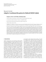
Figure 1: Block diagram of the LT quantization of LSF parameters.
The decoder (bottom part of the diagram) is actually included in
the encoder, since the algorithm for estimating the order P and
the LT model coefficients is an analysis-by-synthesis process (see
Section 3.2).
case in usual coding techniques) using VQ. The indexes of
the P + 1 codewords are transmitted. At the decoder, the
corresponding quantized vectors are gathered in a I
×(P +1)
matrix denoted
ω
(I),(J)
, and the DCM coefficient matrix is
estimated by applying (7) with this quantized reduced set of
LSF vectors instead of the unquantized reduced set:

C = ω
(I),(J)
Q

T

QQ
T

−1
. (8)
Eventually, the “quantized” LSF vectors at the original K
indexes n
k
are given by applying a variant of (3) using (8):
ω
(I),(K)
=

CM. (9)
Note that the resulting LSF vectors, which are the column
of the above matrix, are abusively called the “quantized”
LSF vectors, although they are not directly generated by
VQ. This is because they are the LSF vectors used at the
decoder for signal reconstruction. Note also that (8)implies
that the matrix Q, or alternately the vector J, is available at
the decoder. In this study, the P + 1 positions are regularly
spaced in the considered speech section (with rounding to
the nearest integer if necessary). Thus J can be generated at
the decoder and need not be transmitted. Only the size K of
the sequence and the order P must be transmitted in addition
to the LSF vector codewords. A quantitative assessment of the
corresponding additional bit rate is given in Section 4.4.We
will see that it is very small compared to the bit rate gain

provided by the LT coding method. The whole process is
summarized in Figure 1.
3.2. Iterative Estimation of Model Order. In this subsection,
we present the iterative algorithm that is used to estimate the
optimal DCM order P for each sequence of K LSF vectors.
For this, a performance criterion for the overall process is
first defined. This performance criterion is the usual Average
Spectral Distortion (ASD) measure, which is a standard in
LPC-based speech coding [28]:
ASD
=





1
K
K

k=1
100
π

π
0

log
10
P

k
(e
jω
) − log
10

P
k
(e
jω
)

2
dω,
(10)
where P
k
(e
jω
)and

P
k
(e
jω
) are the LPC power spectra
corresponding to the original and quantized LSF vectors,
EURASIP Journal on Audio, Speech, and Music Processing 5
respectively, for frame k (remind that K is the size of the
quantized LSF vector sequence). In practice, the integral in

(10) is calculated using a 512-bins FFT.
For a given quantizer, an ASD target value, denoted
ASD
max
, is set. Then, starting with P = 1, the complete
process of Section 3.1 is applied. The ASD between the orig-
inal and quantized LSF vector sequences is then calculated.
If it is below ASD
max
, the order is fixed to P, otherwise, P is
increased by one and the process is repeated. The algorithm
is terminated for the first value of P assuming that ASD is
below ASD
max
, or otherwise, for P = K − 2sincewemust
assume P +1<K. All this can be formalized by the following
algorithm:
(1) choose a value for ASD
max
.SetP = 1;
(2) apply the LT coding process of Section 3.1, that is:
(i) calculate C with (4),
(ii) calculate J
= f (P,N),
(iii) calculate ω
(I),(J)
with (6),
(iv) quantize ω
(I),(J)
to obtain ω

(I),(J)
,
(v) calculate
ω
(I),(K)
by combining (9)and(8);
(3) calculate ASD between ω
(I),(K)
and ω
(I),(K)
with (10);
(4) if ASD > ASD
max
and P<K−2, set P ← P +1,and
go to step (2), else (if ASD < ASD
max
or P = K −2),
terminate the algorithm.
3.3. Quantizers. In this subsection, we present the quantizers
that are used to quantize the reduced set of LSF vectors in
step (2) of the above algorithm. As briefly mentioned in the
introduction, vector quantization (VQ) has been generalized
for LSF coefficients quantization in modern speech coders
[1, 3, 4]. However, for high-quality coding, basic single-
stage VQ is generally limited by codebook storage capacity,
search complexity and training procedure. Thus different
suboptimal but still efficient schemes have been proposed to
reduce complexity. For example, split-VQ, which consists of
splitting the vectors into several sub-vectors for quantization,
has been proposed at 24 bits/frames and offered coding

transparency [28].
7
In this study, we used multistage VQ (MS-VQ)
8
which
consists in cascading several low-resolution VQ blocks [29,
30]:Theoutputofablockisanerrorvectorwhichis
quantized by the next block. The quantized vectors are
reconstructed by adding the outputs of the different blocks.
Therefore, each additional block increases the quantization
accuracy while the global complexity (in terms of codebook
generation and search) is highly reduced compared to a
single-stage VQ with the same overall bit rate. Also, different
quantizers were designed and used for voiced and unvoiced
LSF vectors, as in, for example, [31]. This is because we want
to benefit from the V/UV signal segmentation to improve
the quantization process by better fitting the general trends
of voiced or unvoiced LSFs. Detailed information on the
structure of the MS-VQ used in this study, their design, and
their performances, is given in Section 4.3.
3.4. Rate-Distortion Considerations. Now that the long-term
coding method has been presented, it is interesting to derive
an expression of the error between the original and quantized
LSF matrices. Indeed, we have
ω
(I),(K)
−ω
(I),(K)
=


CM −ω
(I),(K)
. (11)
Combining (11)with(8), and introducing q
(I),(J)
= ω
(I),(J)
−

ω
(I),(J)
, basic algebra manipulation leads to:
ω
(I),(K)
−ω
(I),(K)
= ω
(I),(K)
−ω
(I),(K)
+ q
(I),(J)
Q
T

QQ
T

−1
M.

(12)
Equation (12) shows that the overall quantization error on
LSF vectors can be seen as the sum of the contributions
of the LT modeling and the quantization process. Indeed,
on the right side of (12), we have the LT modeling error
defined as the difference between the modeled and the
original LSF vectors sequence. Additionally, q
(I),(J)
is the
quantization error of the reduced set of LSF vectors. It
is “spread” over the K original time indexes by a (P +
1)
× K linear transformation built from matrices M and
Q. The modeling and quantization errors are independent.
Therefore, the proposed method will be efficientifthebitrate
gain resulting from quantizing only the reduced set of P +1
LSF vectors (compared to quantizing the whole K vectors in
frame-by-frame quantization) compensate for the loss due to
the modeling.
In the proposed LT LSF coding method, the bit rate b for
a given section of speech is given by b
= ((P +1)×r)/(K ×h),
where r is the resolution of the quantizer (in bits/vector) and
h is the hop size of the LSF analysis window (h
= 20 ms).
Since the LT coding scheme is an intrinsic variable-rate
technique, we also define an average bit rate, which results
from encoding a large number of LSF vector sequences:
b
=


M
m=1
(
P
m
+1
)

M
m=1
K
m
×
r
h
, (13)
where m indexes each sequence of LSF vectors of the
considered database, M being the number of sequences. In
the LT coding process, increasing the quantizer resolution
does not necessarily increase the bit rate, as opposed to usual
coding methods, since it may lead to decrease the number
of LT model coefficients (for the same overall ASD target).
Therefore, an optimal LT coding configuration is expected
to result from a trade-off between quantizer resolution and
LT modeling accuracy. In Section 4.4,weprovideextensive
distortion-rate results by testing the method on a large
speech database, and varying both the resolution of the
quantizer and the ASD target value.
4. Experiments

In this section, we describe the set of experiments that were
conducted to test the long-term coding of LSF trajectories.
We first briefly describe in Section 4.1 the 2D-transform cod-
ing techniques [18, 19] that we implemented in parallel for
comparison with the proposed technique. The database used
6 EURASIP Journal on Audio, Speech, and Music Processing
in the experiments is presented in Section 4.2. Section 4.3
presents the design of the MS-VQ quantizers used in the LT
coding algorithm. Finally, in Section 4.4, the results of the
LSF long-term coding process are presented.
4.1. 2D-Transform Coding Reference Methods. As briefly
mentioned in the introduction, the basic principle of the
2D-transform coding methods consists in applying either
a 2D-DCT or a Karhunen-Loeve Transform (KLT) on the
I
× K LSF matrices. In contrast to the present study, the
resulting transform coefficients are directly quantized using
scalar quantization (after being normalized though). Bit
allocation tables, transform coefficients mean and variance,
and optimal (non-uniform) scalar quantizers are determined
during a training phase applied on a training corpus of data
(see Section 4.2): Bit allocation among the set of transformed
coefficients is determined from their variance [32] and the
quantizers are designed using the LBG algorithm [33] (see
[18, 19] for details). This is done for each considered tempo-
ral size K, and for a large range of bit rates (see Section 4.4).
4.2. Database. We used American English sentences from the
TIMIT database [34]. The signals were resampled at 8 kHz
and low- and high-pass filtered at the 300–3400 Hz telephone
band.TheLSFvectorswerecalculatedevery20msusingthe

autocorrelation method, with a 30 ms Hann window (hence
a 33% overlap),
9
high-frequency pre-emphasis with the filter
H(z)
= 1 − 0.9375z
−1
, and 10 Hz-bandwidth expansion.
The voiced/unvoiced segmentation was based on the TIMIT
label files which contain the phoneme labels and boundaries
(given as sample indexes) for each sentence. A LSF vector was
classified as voiced if at least 25% of the analysis frame was
part of a voiced phoneme region. Otherwise, it was classified
as an unvoiced LSF vector.
Eight sentences of each of 176 speakers (half male and
half female) from the eight different dialect regions of the
TIMIT database were used for building the training corpus.
Thisrepresentsabout47mnofvoicedspeechand16mn
of unvoiced speech. This resulted in 141,058 voiced vectors
from 9,744 sections, and 45,220 unvoiced LSF vectors from
9,271 sections. This corpus was used to design the MS-VQ
quantizers used in the proposed LT coding technique (see
Section 4.3). It was also used to design the bit allocation
tables and associated optimal scalar quantizers for the 2D-
transform coefficients of the reference methods.
10
In parallel, eight other sentences from 84 other speakers
(also 50% male, 50% female, and from the eight dialect
regions) were used for the test corpus. It contains 67,826
voiced vectors from 4,573 sections (about 23 mn of speech),

and 22,242 unvoiced vectors from 4,351 sections (about 8 mn
of speech). This test corpus was used to test the LT coding
method, and compare it with frame-by-frame VQ and the
2D-transform methods.
The histogram of the temporal size K of the LSF (voiced
and unvoiced) sequences for both training and test corpus
are given on Figure 2. Note that the average size of an
unvoiced sequence (about 5 vectors
≈100 ms) is significantly
smaller than the average size of a voiced sequence (about 15
vectors
≈300 ms). Since there are almost as many voiced and
0
100
200
300
400
500
600
700
Number of occurrences
10 20 30 40 50 60 70 80 90 100
Size of LSF sequences
Voiced speech sections
(a)
0
200
400
600
800

1000
1200
1400
1600
Number of occurrences
5 10152025
Size of LSF sequences
Unvoiced speech sections
(b)
Figure 2: Histograms of the size of the speech sections of the
training (black) and test (white) corpus, for the voiced (a) and
unvoiced (b) sections.
unvoiced sections, the average number of voiced or unvoiced
sections per second is about 2.5.
4.3. MS-VQ Codebooks Design. As mentioned in Section 3.3,
for quantizing the reduced set of LSF vectors, we imple-
mented a set of MS-VQ for both voiced LSF vectors and
unvoiced LSF vectors. In this study, we used two-stage and
three-stage quantizers, with a resolution ranging from 20
to 36 bits/vector, with a 2 bits step. Generally, a resolution
of about 25 bits/vector is necessary to provide transparent
or “close to transparent” quantization, depending on the
structure of the quantizer [29, 30]. In parallel, it was reported
in [31] that significantly fewer bits were necessary to encode
unvoiced LSF vectors compared to voiced LSF vectors.
Therefore, the large range of resolution that we used allowed
EURASIP Journal on Audio, Speech, and Music Processing 7
to test a wide set of configurations, for both voiced and
unvoiced speech.
The design of the quantizers was made by applying

the LBG algorithm [33] on the (voiced or unvoiced)
training corpus described in Section 4.1, using the perceptual
weighted Euclidian distance between LSF vectors proposed in
[28]. The two/three-stage quantizers are obtained as follows.
The LBG algorithm is first used to design the first codebook
block. Then, the difference between each LSF vector of the
training corpus and its associated codeword is calculated.
The overall resulting set of vectors is used as a new training
corpus for the design of the next block, again with the
LBG algorithm. The decoding of a quantized LSF vector
is made by adding the outputs of the different blocks. For
resolutions ranging from 20 to 24, two-stage quantizers were
designed, with a balanced bit allocation between stages, that
is, 10-10, 11-11, and 12-12. For resolutions within the range
26–36, a third stage was added with 2 to 12 bits. This is
because computational considerations limit the resolution
of each block to 12 bits. Note that the ms structure does
not guarantee that the quantized LSF vector is correctly
conditioned (i.e., in some cases, LSF pairs can be too close
to each other or even permuted). Therefore, a regularization
procedure was added to ensure correct sorting and a minimal
distance of 50 Hz between LSFs.
4.4. Results. In this subsection, we present the results
obtained by the proposed method for LT coding of LSF
vectors. We first briefly present a typical example of a sen-
tence. We then give a complete quantitative assessment of the
method over the entire test database, in terms of distortion-
rate. Comparative results obtained with classic frame-by-
frame quantization and the 2D-transform coding techniques
are provided. Finally, we give perceptual evaluation of the

proposed method.
4.4.1. A Typical Example of a TIMIT Sentence. We fi rst
illustrate the behavior of the algorithm of Section 3.2 on
a given sentence of the corpus. The sentence is “Elderly
people are often excluded” pronounced by a female speaker. It
contains five voiced sections and four unvoiced sections (see
Figure 3). In this experiment, the target ASD
max
was 2.1 dB
for the voiced sections, and 1.9 dB for the unvoiced sections.
For the voiced sections, setting r
= 20, 22 and 24 bits/vector
respectively, leads to a bit rate of 557.0, 515.2 and 531.6 bits/s
respectively, for an actual ASD of 1.99, 2.01 and 1.98 dB
respectively. The corresponding total number of model
coefficients is 44, 37 and 35 respectively, to be compared
with the total number of voiced LSF vectors which is 79.
This illustrates the fact that, as mentioned in Section 3.4,
for the LT coding method, the bit rate does not necessarily
decrease as the resolution increases, since the number of
model coefficients also varies. In this case, r
= 22 bits/s seems
to be the best choice. Note that in comparison, the frame-by-
frame quantization provides 2.02 dB of ASD at 700 bits/s. For
the unvoiced sections, the best results are obtained with r
=
20 bits/vector: we obtain 1.82 dB of ASD at 620.7 bits/s (the
frame-by-frame VQ provides 1.81 dB at 700 bits/s).
Speech signal
2000 4000 6000 8000 10000 12000 14000 16000

Time (sample index)
V1 V2 V3 V4 V5
U1 U2 U3 U4
(a)
0.5
1
1.5
2
2.5
LSF parameters (rad/s)
10 20 30 40 50 60 70 80 90 100
Time (frame index)
(b)
Figure 3: Sentence “Elderly people are often excluded”fromthe
TIMIT database, pronounced by a female speaker. (a) The speech
signal; the nth voiced/unvoiced section is denoted V/U n; the total
number of voiced (resp., unvoiced) LSF vectors is 79 (resp., 29). The
vertical lines define the V/U boundaries given by the TIMIT label
files. (b) LSF trajectories; solid line: original LSF vectors; dotted line:
LT-coded LSF vectors with ASD
max
= 2.1 dB for the voiced sections
(r
= 22 bits/vectors) and ASD
max
= 1.9 dB for the unvoiced sections
(r
= 20 bits/vectors) (see the text). The vertical lines define the V/U
boundaries between analysis frames, that is, the limits between LT-
coded sections (the analysis frame is 30 ms long with a 20 ms hop

size).
We can s ee on Figure 3 the corresponding original and
LT-coded LSF trajectories. This figure illustrates the ability
of the LT model of LSF trajectories to globally fit the original
trajectories, even if the model coefficients are calculated from
the quantized reduced set of LSF vectors.
4.4.2. Average Distortion-Rate Results. In this subsection,
we generalize the results of the previous subsection by (i)
varying the ASD target and the MS-VQ resolution r within
a large set of values, (ii) applying the LT coding algorithm
on all sections of the test database, and averaging the bit rate
(13) and the ASD (10) across either all 4,573 voiced sections
or all 4,351 unvoiced sections of the test database, and (iii)
comparing the results with the ones obtained with the 2D-
transform coding methods and the frame-by-frame VQ.
As already mentioned in Section 4.2, the resolution range
for the MS-VQ quantizers used in LT coding is within 20 to
8 EURASIP Journal on Audio, Speech, and Music Processing
20
22
14
16
18
20
26
28
28
30
32
34

36
24
30
1
1.2
1.4
1.6
1.8
2
2.2
2.4
ASD (dB)
400 500 600
Long-term coding
Frame-by-frame
quantization
700 800 900 1000 1100 12001300 1400
Average bit-rate (bits/s)
Figure 4: Average spectral distortion (ASD) as a function of the
average bit rate, calculated on the whole voiced test database, and
for both the LSF LT coding and frame-by-frame LSF quantization.
The plotted numbers are the resolutions (in bits/vector). For each
resolution, the different points of each LT-coding curve cover the
range of the ASD target.
36 bits/vector. The ASD target was being varied from 2.6 dB
to a minimum value with a 0.2 dB step. The minimum value
is 1.0 dB for r
= 36, 34, 32 and 30 bits/vector, and then it
is increased by 0.2dB each time the resolution is decreased
by2bits/vector(itisthus1.2dBforr

= 28 bits/vector,
1.4 dB for r
= 26 bits/vector, and so on). In parallel, the
distortion-rate values were also calculated for usual frame-
by-frame quantization using the same quantizers than in the
LT coding process, and using the same test corpus. In this
case, the resolution range was extended to lower values for
a better comparison. For the 2D-transform coding methods,
the temporal size was varied from 1 to 20 for voiced LSFs,
and from 1 to 10 for unvoiced LSFs. This choice was made
after the histograms of Figure 2 and after considerations on
computational limitations.
11
It is coherent with the values
considered in [19]. We calculated the corresponding ASD
for the complete test corpus, and for seven values of the
optimal scalar quantizers resolution: 0.75, 1, 1.25, 1.5, 1.75,
2.0 and 2.25 bits/parameter. This corresponds to 375, 500,
625, 750, 875, 1,000 and 1,125 bits/s, respectively, (since the
hop size is 20 ms). We also calculated for each of these
resolutions a weighted average value of the spectral distortion
(ASD), the weights being the bins of the histogram of
Figure 2 (for the test corpus) normalized by the total size
of the corpus. This enables one to take into account the
distribution of the temporal size of the LSF sequences in
the rate-distortion relationship, for a fair comparison with
the proposed LT coding technique. This way, we assume
that both the proposed method and 2D-transform coding
methods work with the same “adaptive” temporal-block
configuration.

The results are presented in Figures 4 and 5 for the voiced
sections, and in Figures 6 and 7 for the unvoiced sections. Let
us begin the analysis of the results with the voiced sections.
Figure 4 displays the results of the LT coding technique in
terms of ASD as a function of the bit rate. Each one of
the curves on the left of the figure corresponds to a fixed
MS-VQ resolution (which value is plotted), the ASD target
being varied. It can be seen that the different resolutions
provide an array of intertwined curves, each one following
the classic general rate-distortion relationship: an increase of
the ASD goes with a decrease of the bit rate. These curves are
generally situated on the left of the curve corresponding to
the frame-by-frame quantization, which is also plotted. They
thus generally correspond to smaller bit rates. Moreover, the
gain in bit rate for approximately the same ASD can be very
large, depending on the considered region and the resolution
(see more details below). In a general manner, the way the
curves are intertwined involves that increasing the resolution
of the MS-VQ quantizer makes the bit rate increase for the
left upper region of the curves, but it is no more the case in
the right lower region, after the “crossing” of the curves. This
illustrates the specific trade-off that must be tuned between
quantization accuracy and modeling accuracy, as mentioned
in Section 3.4. The ASD target value has a strong influence
on this trade-off. For a given ASD level, the lower bit rate
is obtained with the leftmost point, which depends on the
resolution. The set of optimal points for the different ASD
values, that is, the left-down envelope of the curves, can be
extracted and it forms what will be referred to as the optimal
LT coding curve.

For easier comparison, we report this optimal curve
on Figure 5, and we also plot on this figure the results
obtained with the 2D-DCT and KLT transform coding
methods (and also again the frame-by-frame quantization
curve). The curves of the 2D-DCT transform coding are
given for the temporal size 2, 5, 10 and 20, and also for
the “adaptive” curve (i.e., the values averaged according to
the distribution of the temporal size) which is the main
reference in this variable-rate study. We can see that for
the 2D-DCT transform coding, the longer is the temporal
size, the lower is the ASD. The average curve is between the
curves corresponding to K
= 5andK = 10. For clarity, the
KLT transform coding curve is only given for the adaptive
configuration. This curve is about 0.05 to 0.1 dB below
the adaptive 2D-DCT curve, which corresponds to about
2-3 bits/vector savings, depending on the bit rate (this is
consistent with the optimal character of the KLT and with
the results reported in [19]).
We c an see on Figure 5 that the curves of the 2D-
transform coding techniques are crossing the optimal LT
coding curve from top-left to bottom-right. This implies
that for the higher part of the considered bit-range (say
above about 900 bits/s) the 2D-transform coding techniques
provide better performances than the proposed method.
These performances tend toward the 1 dB transparency
bound for bit rates above 1 kbits/s, which is consistent with
the results of [18]. With the considered configuration, the
LT coding technique is limited to about 1.1dB of ASD, and
the corresponding bit rate is not competitive with the bit

rate of the 2D-transform techniques (it is even comparable
to the simple frame-by-frame quantization over 1.2 kbits/s).
In contrast, for lower bit rates, the optimal LT coding
EURASIP Journal on Audio, Speech, and Music Processing 9
1
1.2
1.4
1.6
1.8
2
2.2
2.4
2.6
2.8
3
ASD (dB)
400 600
Optimal
long-term
quantization
2D-DCT transform
coding
Adaptive 2D-DCT
transform coding
Adaptive KLT
transform coding
Frame-by-frame
quantization
800 1000 1200 1400
Average bit-rate (bits/s)

Figure 5: Average spectral distortion (ASD) as a function of the
average bit rate, calculated on the whole voiced test database, and
for LSF optimal LT coding (continuous line, black points, on the
left); Frame-by-frame LSF quantization (continuous line, black
points, on the right); 2D-DCT transform coding (dashed lines, grey
circles)for,fromtoptobottom,K
= 2, 5, 10, and 20; adaptive 2D-
DCT transform coding (continuous line, grey circles); and adaptive
2D-KLT transform coding (continuous line, grey diamonds).
20
22
24
26
28
12
30
32
34
36
20
22
24
1
1.2
1.4
1.6
1.8
2
ASD (dB)
400 500 600

Long-term
coding
Frame-by-frame
quantization
700 800 900 1000 1100 1200 1300
Average bit-rate (bits/s)
Figure 6: Same as Figure 4, but for the unvoiced test database.
technique clearly outperforms both 2D-transform methods.
For example, at 2.0 dB of ASD, the bit rates of the LT,
KLT, and 2D-DCT coding methods are about 489, 587, and
611 bits/s respectively. Therefore, the bit rate gain provided
by the LT coding technique over the KLT and 2D-DCT
techniques is about 98 bits/s (i.e., 16.7%) and 122 bits/s (i.e.,
20%) respectively. Note that for such ASD value, the frame-
by-frame VQ requires about 770 bits/s. Therefore, compared
to this method, the relative gain in bit rate of the LT coding
is about 36.5%. Moreover, since the slope of the LT coding
curve is smaller than the slope of the other curves, the
relative gain in bit rate (or in ASD) provided by the LT
coding significantly increases as we go towards lower bit
rates. For instance, at 2.4 dB, we have about 346 bits/s for
the LT coding, 456 bits/s for the KLT, 476bits/s for the 2D-
DCT, and 630 bits/s for the frame-by-frame quantization.
The relative bit rate gains are respectively 24.1% (110 out of
456), 27.3% (130 out of 476), and 45.1% (284 out of 630).
IntermsofASD,wehaveforexample1.76dB,1.90dB,
and 1.96 dB respectively for the LT coding, the KLT, and the
2D-DCT at 625 bits/s. This represents a relative gain of 7.4%
and 10.2% for the LT coding over the two 2D-transform
coding techniques. At 375 bits/s this gain reaches respectively

15.8% and 18.1% (2.30 dB for the LT coding, 2.73 dB for the
KLT, and 2.81 dB for the 2D-DCT).
For unvoiced sections, the general trends of the LT
quantization technique discussed in the voiced case can be
retrieved in Figure 6. However, at a given bit rate, the ASD
obtained in this case is generally slightly lower than in the
voiced case, especially for the frame-by-frame quantization.
This is because unvoiced LSF vectors are easier to quantize
than voiced LSF vectors, as pointed out in [31]. Also, the
LT coding curves are more “spread” than for the voiced
sections of speech. As a result, the bit rates gains compared
to the frame-by-frame quantization are positive only below,
say, 900 bits/s, and they are generally lower than in the
voiced case, although they remain significant for the lower
bit rates. This can be seen more easily on Figure 7,where
the optimal LT curve is reported for unvoiced sections. For
example, at 2.0 dB the LT quantization bit rate is about
464 bits/s, while the frame-by-frame quantizer bit rate is
about 618 bits/s (thus the relative gain is 24.9%). Compared
to the 2D-transform techniques, the LT coding technique
is also less efficient than in the voiced case. The “crossing
point” between LT coding and 2D-transform coding is here
at about
{700–720 bits/s, 1.6 dB}. On the right of this point,
the 2D-transform techniques clearly provide better results
than the proposed LT coding technique. In contrast, below
700 bits/s, the LT coding provides better performances, even
if the gains are lower than in the voiced case. An idea of the
maximum gain of LT coding over 2D-transform coding is
given at 1.8 dB: the LT coding bit rate is 561 bits/s, although it

is 592 bits/s for the KLT, and 613 bits/s for the 2D-DCT (the
corresponding relative gains are 5.2% and 8.5%, resp.).
Let us close this subsection with a calculation of the
approximate bit rate which is necessary to encode the
{K, P}
pair (see Section 3.1). It is a classical result that any finite
alphabet α can be encoded with a code of average length
L,withL<H(α)+1,whereH(α) is the entropy of the
alphabet [1]. We estimated the entropy of the set of
{K, P}
pairs obtained on the test corpus after termination of the LT
coding algorithm. This was done for the set of configurations
corresponding to the optimal LT coding curve. Values within
the interval
{6.38, 7.41} and {3.91, 4.60} were obtained for
the voiced sections and unvoiced sections respectively. Since
the average number of voiced or unvoiced sections is about
2.5 per second (see Section 4.2), the additional bit rate is
about 7
× 2.5 = 17.5 bits/s for the voiced sections and about
4.3
× 2.5 = 10.75 bits/s for the unvoiced sections. Therefore,
it is quite small compared to the bit rate gain provided by
the proposed LT coding method over the frame-by-frame
10 EURASIP Journal on Audio, Speech, and Music Processing
1
1.2
1.4
1.6
1.8

2
2.2
ASD (dB)
Optimal
long-term
quantization
2D-DCT transform
coding
Adaptive 2D-DCT
transform coding
Adaptive KLT
transform coding
Frame-by-frame
quantization
Average bit-rate (bits/s)
300 400 500 600 700 800 900 1000 1100 1200 1300
Figure 7: Same as Figure 5, but for the unvoiced test database. The
results of the 2D-DCT transform coding (dashed lines, grey circles)
are plotted for, from top to bottom, K
= 2, 5, and 10.
quantization. Besides, the 2D-transform coding methods
require the transmission of the size K of each section.
Following the same idea, the entropy for the set of K values
was found to be 5.1bits for the voiced sections, and 3.4 bits
for the unvoiced section. Therefore, the corresponding
coding rates are 5.1
× 2.5 = 12.75 bits/s and 3.4 × 2.5 =
8.5 bits/s respectively. The difference between encoding K
and the pair
{K, P}is less than 5 bits/s in any case. This shows

that (i) the values of K and P are significantly correlated,
and (ii) because of this correlation, the additional cost for
encoding P in addition to K is very small compared to the bit
rate difference between the proposed method and the 2D-
transform methods within the bit rate range of interest.
4.4.3. Listening Tests. To confirm the efficiency of the long-
term coding of LSF parameters from a subjective point of
view, signals with quantized LSFs were generated by filtering
the original signals with the filter F(z)
= A(z)/

A(z), where

A(z) is the LPC analysis filter derived from the quantized
LSF vector, and A(z) is the original (unquantized) LPC filter
(this implies that the residual signal is not modified). The
sequence of

A(z) filters was generated with both the LT
method and 2D-DCT transform coding. Ten sentences of
TIMIT were selected for a formal listening test (5 by a male
speaker and 5 by a female speaker, from different dialect
regions). For each of them, the following conditions were
verified for both voiced and unvoiced sections: (i) the bit
rate was lower than 600 bits/s; (ii) the ASD was between
1.8 dB and 2.2 dB; (iii) the ASD absolute difference between
LT-coding and 2D-DCT coding was less than 0.02 dB; and
(iv) the LT coding bit rate was at least 20% (resp., 7.5%)
lower than the 2D-DCT coding bit rate for the voiced (resp.,
unvoiced) sections. Twelve subjects with normal hearing

listened to the 10 pairs of sentences coded with the two
methods and presented in random order, using a high-
quality PC soundcard and Sennheiser HD280 Headphones,
in a quiet environment. They were asked to make a forced
choice (i.e., perform an A-B test), based on the perceived best
quality.
The overall preference score across sentences and subjects
is 52.5% for the long-term coding versus 47.5% for the 2D-
DCT transform coding. Therefore, the difference between
the two overall scores does not seem to be significant.
Considering the scores sentence by sentence reveals that,
for two sentences, the LT coding is significantly preferred
(83.3% versus 16.7%, and 66.6% versus 33.3%). For one
other sentence, the 2D-DCT coding method is significantly
preferred (75% versus 25%). In those cases, both LT coded
signal and 2D-DCT coded signal exhibit audible (although
rather small) artifacts. For the seven other sentences, the
scores vary between 41.7%–58.3% to the inverse 58.3%–
41.7%, thus indicating that for these sentences, the two
methods provide very close signals. In this case, and for both
methods, the quality of the signals, although not transparent,
is quite fairly good for such low rates (below 600 bits/s):
the overall sounding quality is preserved, and there is no
significant artifact.
These observations are confirmed by extended informal
listening tests on many other signals of the test database: It
has been observed that the quality of the signals obtained
by the LT coding technique (and also by the 2D-DCT
transform coding) at rates as low as 300
−500 bits/s varies

a lot. Some coded sentences are characterized by quite
annoying artifacts, whereas some others exhibit surprisingly
good quality. Moreover, in many cases, the strength of the
artifacts does not seem to be directly correlated with the
ASD value. This seems to indicate that the quality of very-
to-ultra low bit rate LSF quantization may largely depend
on the signal itself (e.g., speaker and phonetic content). The
influence of such factors is beyond the scope of this paper,
but it should be considered more carefully in future works.
4.4.4. A Few Computational Considerations. The complete LT
LSF coding and decoding process is done in approximately
half real-time using MATLAB on a PC with a processor at
2.3 GHz (i.e., 0.5 s is necessary to process 1 s of speech).
12
Experiments were conducted with the “raw” exhaustive
search of optimal order P in the algorithm of Section 3.2.A
refined (e.g., dichotomous) search procedure would decrease
the computational cost and time by a factor of about 4 to
5. Therefore, an optimized C implementation would run
within several ranges of order below real-time. Note that the
decoding time is only a small fraction (typically 1/10 to 1/20)
of the coding time since decoding consists in applying only
(8)and(9) only once, using the reduced set of decoded LSF
vectors and decoded
{K, P} pair.
5. Summary and Perspectives
In this paper, a variable-rate long-term approach to LSF
quantization has been proposed for offline or large-delay
speech coding. It is based on the modeling of the time-
trajectories of LSF parameters with a Discrete Cosine model,

combined with a “sparse” vector quantization of a reduced
set of LSF vectors. An iterative algorithm has been shown to
provide joint efficient shaping of the model and estimation of
EURASIP Journal on Audio, Speech, and Music Processing 11
its optimal order. As a result, the method generally provides
a very large gain in bit rate (up to 45%) compared to short
term (frame-by-frame) quantization, at an equivalent coding
quality. Also, for the lower range of tested bit rates (i.e.,
below 600–700 bits/s), the method compares favorably with
transform coding techniques that also exploit the interframe
correlationofLSFsacrossmanyframes.Thishasbeen
demonstrated by extensive distortion/rate benchmark and
listening tests. The bit rate gain is up to about 7.5% for
unvoiced speech, and it is up to about 25% for voiced
speech, depending on coding accuracy. Of course, at the
considered low bit rates, the ASD is significantly above the
1.0 dB bound which is correlated with transparency quality.
However, the proposed method provides a new bound of
attainable performances for LSF quantization at very- to
ultra-low bit rates. It can also be used as a first stage in a
refined LSF coding scheme at higher rates: the difference
between original and LT-coded LSF can be coded by other
techniques after that the long-term interframe correlation
has been removed.
It must be mentioned here that although efficient, the
MS-VQs used in this study are not the best quantizers
available. For instance, we have not used fully optimized
(i.e., using treillis search as in [30]) MS-VQ, but basic (i.e.,
sequential search) MS-VQ. Also, more sophisticated frame-
wise methods have been proposed to obtain transparent

LSF quantization at rates lower than the ones required
for MS-VQ, but at the cost of increased complexity [35,
36]. Refined versions of split-VQ are also good candidates
for improved performances. We restricted ourselves with
a relatively simple VQ technique because the goal of the
present study was primarily to show the interest of the
long-term approach. Therefore, it is very likely that the
performances of the proposed LT coding algorithm can be
significantly improved by using high-performance (but more
complex) quantizers,
13
since the reduced set of LSF vectors
may be quantized with lower ASD/resolution compared to
the MS-VQ. In contrast, it seems very difficult to improve
the performances of the reference 2D-transform methods,
since we used optimal (non-uniform) quantizers to encode
the corresponding 2D coefficients.
As mentioned before, the analysis settings have been
shown to noticeably influence the performance of the
proposed method. As pointed out in [13], “it is desirable
for the formant filter parameters to evolve slowly, since
their [short-term] fluctuations may be accentuated under
quantization, creating audible distortions at update instants”.
Hence it may be desirable to carefully configure the analysis,
or to pre-process the LSF with a smoothing method (such as
[13, 14]oradifferent one) before long-term quantization, to
obtain trajectories freed from undesirable local fluctuations
partly due to analysis (see Figure 3). This is likely to enable
the proposed fitting algorithm to significantly lower the LT
model order and hence lower the bit rate, without impair-

ing signal quality. A deeper investigation of this point is
needed.
Beyond those potential improvements, future work may
focus on the elaboration of several complete speech coders
functioning at very- to ultra-low bit rates and exploiting the
long-term approach. This requires an appropriate adaptation
of the proposed algorithm to the coding of the excitation
(residual signal). For example, ultra-low bit rate coding
with acceptable quality may be attainable with the long-
term coding of basic excitation parameters such as funda-
mental frequency, voicing frequency (i.e., the frequency that
“separates” the voiced region and the unvoiced region for
mixed V/UV sounds), and corresponding gains. Also, we
intend to test the proposed long-term approach within the
framework of (unit-based concatenative) speech synthesis.
As mentioned in Section 2, the long-term model that is used
here to exploit the predictability of LSF trajectories can also
be directly used for time interpolation of those trajectories
(a property that is not assumed by 2D-transform coding; see
Endnote 5). In other words, the proposed method offers an
efficient framework for direct combination of decoding and
time interpolation, as required for speech transformation in
(e.g., TTS) synthesis systems. It can be used to interpolate
LSF (and also source parameters) “natural” trajectories, to be
compared in future works with more or less complex existing
interpolation schemes. Note that the proposed method is
particularly suitable for unit-based synthesis, since it is
naturally frame length- and bitrate-adaptive. Therefore, an
appropriate mapping between speech units and long-term
frames can be defined.

14
As suggested by [13], the interaction
between filter parameters and source parameters should
be carefully examined within this long-term coding and
interpolating framework.
Endnotes
1. The differential VQ and other schemes such as pre-
dictive VQ and finite-state VQ can be seen as spe-
cial cases of recursive VQ [2, 10], depending on
the configuration.
2. In the following, the term “long-term” refers to con-
sidering long sections of speech, including several to
many short-term frames of about 20 ms. Hence, it has
adifferent meaning than in the “long-term (pitch)
predictor” of speech coders.
3. The V/UV segmentation is compliant with the expecta-
tion of somewhat “coherent” LSF trajectories on a given
long-term section. Indeed, it is well known that these
parameters have a different general behavior for voiced
or unvoiced sounds (see, e.g., [31]).
4. In the following, all vectors of consecutive values in
time are row vectors, while vectors of simultaneous
values taken at a given time instant are column vectors.
Matrices are organized accordingly.
5. This means that, despite of matrix formalism, each line
of (3)isamodeledtrajectoryofoneLSFcoefficient
that is modeled independently of the trajectory of the
other coefficients (except for common model order).
Accordingly, the regression of (4) can be calculated
separately for each line, that is, each set of model

12 EURASIP Journal on Audio, Speech, and Music Processing
coefficients of (1). Hence, the coefficients of C are
time model coefficients. In contrast, 2D-transform
coefficients jointly concentrate both time and frequency
information from data (and those 2D models cannot be
directly interpolated in one dimension).
6. For the fixed-size 10-to-4 conversion of LSF into poly-
nomial coefficients. Let us remind that in the present
study, the K-to-P conversion is of variable dimension.
7. “Coding transparency” means that speech signals syn-
thesized with the quantized and unquantized LSFs are
perceptually undistinguishable.
8. The methods [6–14] exploiting interframe LSF correla-
tion are not pertinent in the present study. Indeed, the
LSF vectors of the reduced set are sparsely distributed in
the considered section of speech, and their correlation is
likely to be poor.
9. The analysis settings have been shown to slightly influ-
ence the performance of the proposed method, since
they can provide successive LSF vectors with slightly
different degrees of correlation. The present settings are
different from the ones used in [24], and they provided
slightly better results. They were partly suggested by
[37]. Also, this suggests that the proposed method is
likely to significantly benefit from a pre-processing of
the LSF with “short-term” smoothing methods, such as
[13, 14] (see Section 5).
10. Note that for the 2D-DCT the coefficients are fixed
whereas they depend on the data for the KLT; thus, for
each tested temporal size, the KLT coefficients are also

determined from the training data.
11. We must ensure (i) a sufficient number of (voiced
or unvoiced) sections of a given size to compute the
corresponding bit allocation tables and optimal scalar
quantizers (and transform coefficients for the KLT), and
(ii) a reasonable calculation time for experiments on
such extended corpus. Note that for the 2D-transform
coding methods, voiced (resp., unvoiced) sequences
larger than 20 (resp., 10) vectors are split into sub-
sequences.
12. In comparison, the adaptive (variable-size) 2D-
transform coding methods require only approximately
1/10th of real-time, hence 1/5th of the proposed
method resource. This is mainly because they do not
require inverse matrix calculation but only direct matrix
products.
13. The proposed method is very flexible in the sense that
it can be directly applied with any type of frame-wise
quantizer.
14. In the present study we used V/UV segmentation (and
adapted coding), but other segmentation, more adapted
to concatenative synthesis, can be considered (e.g.,
“CV” or “VCV”). Alternately, all voiced or all unvoiced
(subsets of) units could be considered in synthesis
system using the proposed method.
References
[1] J. D. Markel and A. H. Gray Jr., Linear Prediction of Speech,
Springer, New York, NY, USA, 1976.
[2] R. M. Gray and A. Gersho, Vector Quantization and Signal
Compression, Kluwer Academic Publishers, Boston, Mass,

USA, 1992.
[3]J.PanandT.R.Fischer,“Vectorquantizationofspeechline
spectrum pair parameters and reflection coefficients,” IEEE
Transactions on Speech and Audio Processing,vol.6,no.2,pp.
106–115, 1998.
[4] P. Hedelin, “Single stage spectral quantization at 20 bits,” in
Proceedings of the IEEE International Conference on Acoustics,
Speech and Signal Processing (ICASSP ’94), pp. 525–528,
Adelaide, Australia, 1994.
[5] N. Sugamura and F. Itakura, “Speech analysis and synthesis
method developed at ACL in NTT—from LPC to LSP,” Speech
Communication, vol. 5, no. 2, pp. 199–215, 1986.
[6] M. Yong, G. Davidson, and A. Gersho, “Encoding of LPC
spectral parameters using switched-adaptive interframe vector
prediction,” in Proceedings of the IEEE International Conference
on Acoustics, Speech and Signal Processing (ICASSP ’88),pp.
402–405, New York, NY, USA, 1988.
[7] F R. Jean and H C. Wang, “Transparent quantization of
speech LSP parameters based on KLT and 2-D-prediction,”
IEEE Transactions on Speech and Audio Processing, vol. 4, no.
1, pp. 60–66, 1996.
[8] C. Tsao and R. M. Gray, “Matrix quantizer design for
LPC speech using the generalized Lloyd algorithm,” IEEE
Transactions on Acoustics, Speech, and Signal Processing, vol. 33,
no. 3, pp. 537–545, 1985.
[9] C. S. Xydeas and C. Papanastasiou, “Split matrix quantization
of LPC parameters,” IEEE Transactions on Speech and Audio
Processing, vol. 7, no. 2, pp. 113–125, 1999.
[10] J. Samuelsson and P. Hedelin, “Recursive coding of spectrum
parameters,” IEEE Transactions on Speech and Audio Process-

ing, vol. 9, no. 5, pp. 492–502, 2001.
[11] A. D. Subramaniam, W. R. Gardner, and B. D. Rao, “Low-
complexity source coding using Gaussian mixture models, lat-
tice vector quantization, and recursive coding with application
to speech spectrum quantization,” IEEE Transactions on Audio,
Speech and Language Processing, vol. 14, no. 2, pp. 524–532,
2006.
[12] S. Subasingha, M. N. Murthi, and S. V. Andersen, “Gaussian
mixture kalman predictive coding of line spectral frequencies,”
IEEE Transactions on Audio, Speech and Language Processing,
vol. 17, no. 2, pp. 379–391, 2009.
[13] M. R. Zad-Issa and P. Kabal, “Smoothing the evolution of the
spectral parameters in linear prediction of speech using target
matching,” in Proceedings of the IEEE International Conference
on Acoustics, Speech and Signal Processing (ICASSP ’97), vol. 3,
pp. 1699–1702, Munich, Germany, 1997.
[14] F. Nord
´
en and T. Eriksson, “Time evolution in LPC spectrum
coding,” IEEE Transactions on Speech and Audio Processing, vol.
12, no. 3, pp. 290–301, 2004.
[15] B. S. Atal, “Efficient coding of LPC parameters by tem-
poral decomposition,” in Proceedings of the IEEE Interna-
tional Conference on Acoustics, Speech and Signal Processing
(ICASSP ’83), vol. 1, pp. 81–84, Boston, Mass, USA, 1983.
[16] A. M. L. Van Dijk-Kappers and S. M. Marcus, “Temporal
decomposition of speech,” Speech Communication, vol. 8, no.
2, pp. 125–135, 1989.
EURASIP Journal on Audio, Speech, and Music Processing 13
[17] Y M. Cheng and D. O’Shaughnessy, “On 450–600 b/s natural

sounding speech coding,” IEEE Transactions on Speech and
Audio Processing, vol. 1, no. 2, pp. 207–220, 1993.
[18] N. Farvardin and R. Laroia, “Efficient encoding of speech
LSP parameters using the discrete cosine transformation,” in
Proceedings of the IEEE International Conference on Acoustics,
Speech and Signal Processing (ICASSP ’89), vol. 1, pp. 168–171,
Glasgow, UK, 1989.
[19]D.J.MudugamuwaandA.B.Bradley,“Optimaltransform
for segmented parametric speech coding,” in Proceedings of the
IEEE International Conference on Acoustics, Speech and Signal
Processing (ICASSP ’98), vol. 1, pp. 525–528, Seattle, Wash,
USA, 1998.
[20] S. Dusan, J. Flanagan, A. Karve, and M. Balaraman, “Speech
coding using trajectory compression and multiple sensors,”
in Proceedings of the International Conference on Speech &
Language Processing, Jeju, South Korea, 2004.
[21] S. Dusan, J. Flanagan, A. Karve, and M. Balaraman, “Speech
compression by polynomial approximation,” IEEE Transac-
tions on Audio, Speech and Language Processing, vol. 15, no. 2,
pp. 387–395, 2007.
[22] L. Girin, M. Firouzmand, and S. Marchand, “Long-term mod-
eling of phase trajectories within the speech sinusoidal model
framework,” in Proceedings of the International Conference on
Speech & Language Processing, Jeju, South Korea, 2004.
[23] L. Girin, M. Firouzmand, and S. Marchand, “Perceptual
long-term variable-rate sinusoidal modeling of speech,” IEEE
Transactions on Audio, Speech and Language Processing, vol. 15,
no. 2, pp. 851–861, 2007.
[24] L. Girin, “Long-term quantization of speech LSF parameters,”
in Proceedings of the IEEE International Conference on Acous-

tics, Speech and Signal Processing (ICASSP ’07), vol. 4, pp. 845–
848, Honolulu, Hawaii, USA, 2007.
[25] L. Girin, M. Firouzmand, and S. Marchand, “Comparing sev-
eral models for perceptual long-term modeling of amplitude
and phase trajectories of sinusoidal speech,” in Proceedings of
the 9th European Conference on Speech Communication and
Technology (Interspeech ’05), pp. 357–360, Lisboa, Portugal,
2005.
[26] T. Galas and X. Rodet, “An improved cepstral method for
deconvolution of source-filter systems with discrete spectra:
application to musical sound signals,” in Proceedings of the
International Computer Music Conference (ICMC ’90), pp. 82–
84, Glasgow, UK, 1990.
[27] O. Capp
´
e, J. Laroche, and E. Moulines, “Regularized estima-
tion of cepstrum envelope from discrete frequency points,”
in Proceedings of the IEEE Workshop on Applications of Signal
Processing to Audio and Acoustics (WASPAA ’95),NewPaltz,
NY, USA, October 1995.
[28] K. K. Paliwal and B. S. Atal, “Efficient vector quantization of
LPC parameters at 24 bits/frame,” IEEE Transactions on Speech
and Audio Processing, vol. 1, no. 1, pp. 3–14, 1993.
[29] N. Phamdo, N. Favardin, and T. Moriya, “Combined
source-channel coding of LSP parameters using multi-stage
vector quantization,” in Proceedings of the IEEE Work-
shop on Speech Coding for Telecommunications, pp. 36–38,
1991.
[30] W. P. LeBlanc, B. Bhattacharya, S. A. Mahmoud, and V.
Cuperman, “Efficient search and design procedures for robust

multi-stage VQ of LPC parameters for 4 kb/s speech coding,”
IEEE Transactions on Speech and Audio Processing,vol.1,no.4,
pp. 373–385, 1993.
[31] R. Hagen, E. Paksoy, and A. Gersho, “Voicing-specific LPC
quantization for variable-rate speech coding,” IEEE Transac-
tions on Speech and Audio Processing, vol. 7, no. 5, pp. 485–494,
1999.
[32] N. S. Jayant and P. Noll, Digital Coding of Waveforms:
Principles and Applications to Speech and Video, Prentice-Hall,
Englewood Cliffs, NJ, USA, 1984.
[33] Y. Linde, A. Buzo, and R. M. Gray, “An algorithm for vector
quantizer design,” IEEE Transactions on Communications
Systems, vol. 28, no. 1, pp. 84–95, 1980.
[34] J. S. Garofolot, L. F. Lamel, W. M. Fisher, et al., TIMIT
Acoustic-Phonetic Continuous Speech Corpus, Linguistic Data
Consortium, Philadelphia, Pa, USA, 1993.
[35] M. A. Ferrer-Ballester and A. R. Figueiras-Vidal, “Efficient
adaptive vector quantization of LPC parameters,” IEEE Trans-
actions on Speech and Audio Processing, vol. 3, no. 4, pp. 314–
317, 1995.
[36] A. D. Subramaniam and B. D. Rao, “PDF optimized paramet-
ric vector quantization of speech line spectral frequencies,”
IEEE Transactions on Speech and Audio Processing, vol. 11, no.
2, pp. 130–142, 2003.
[37] P. Kabal, “Personal communication”.