Báo cáo sinh học: " Research Article Multiplicative Noise Removal via a Novel Variational Model" doc
Bạn đang xem bản rút gọn của tài liệu. Xem và tải ngay bản đầy đủ của tài liệu tại đây (16.95 MB, 16 trang )
Hindawi Publishing Corporation
EURASIP Journal on Image and Video Processing
Volume 2010, Article ID 250768, 16 pages
doi:10.1155/2010/250768
Research Article
Multiplicative Noise Removal via a Novel Variational Model
Li-Li Huang,
1, 2
Liang Xiao,
1
and Zhi-Hui Wei
3
1
School of Computer Science and Technology, Nanjing University of Science and Technology, Nanjing 210094, China
2
Department of Information and Computing Science, Guangxi University of Technology, Liuzhou 545006, China
3
Department of Applied Mathematics, Nanjing University of Science and Technology, Nanjing 210094, China
Correspondence should be addressed to Liang Xiao,
Received 30 March 2010; Revised 5 May 2010; Accepted 2 June 2010
Academic Editor: Lei Zhang
Copyright © 2010 Li-Li Huang et al. This is an open access article distributed under the Creative Commons Attribution License,
which permits unrestricted use, distribution, and reproduction in any medium, provided the original work is properly cited.
Multiplicative noise appears in various image processing applications, such as synthetic aperture radar, ultrasound imaging,
single particle emission-computed tomography, and positron emission tomography. Hence multiplicative noise removal is of
momentous significance in coherent imaging systems and various image processing applications. This paper proposes a nonconvex
Bayesian type variational model for multiplicative noise removal which includes the total variation (TV) and the Weberized TV
as regularizer. We study the issues of existence and uniqueness of a minimizer for this variational model. Moreover, we develop a
linearized gradient method to solve the associated Euler-Lagrange equation via a fixed-point iteration. Our experimental results
show that the proposed model has good performance.
1. Introduction
Image denoising is an inverse problem widely studied in
signal and image processing fields. The problem includes
additive noise removal and multiplicative noise removal. In
many image formation model, the noise is often modeling
as an additive Gaussian noise: given an original image u,
it is assumed that it has been corrupted by some Gaussian
additive noise v. The denoising problem is then to recover
u from the data f
= u + v. There are many effective
methods to tackle this problem. Among the most famous
ones are wavelets approaches [1, 2], stochastic approaches
[3], principal component analysis-based approaches [4, 5],
and variational approaches [6]. We refer the reader to the
literature [7, 8] and references herein for an overview of the
subject.
In this paper, we focus on the issue of multiplicative noise
removal. Specifically, we are interested in the denoising of
SAR images. According to [9] and other references, the noise
in the observed SAR image is a type of multiplicative noise
which is called speckle. And the image formation model is
f
= uv,
(1)
where f is the observed image, u is the original SAR
image, and v is the noise which follows a Gamma Law with
mean one. Speckle is one of the most complex image noise
models. It is signal independent, non-Gaussian, and spatially
dependent. Hence speckle denoising is a very challenging
problem compared with additive Gaussian noise.
Multiplicative noise removal methods have been dis-
cussed in many reports. Popular methods include local
linear minimum mean square error approaches [10, 11],
anisotropic diffusion methods [12–15], and nonlocal means
(NL-means) [16], which will not be addressed in this
paper. We will focus on the variational approach-based
multiplicative noise removal, especially that our researches
will emphasis on TV-based methods.
To the best of our knowledge, there exist several vari-
ational approaches devoted to multiplicative noise removal
problem. The first total variation-based multiplicative noise
removal model (RLO-model) was presented by Rudin et al.
[17], which used a constrained optimization approach with
two Lagrange multipliers. Multiplicative model (AA-model)
with a fitting term derived from a maximum a posteriori
(MAP) was introduced by Aubert and Aujol [18]. Recently,
Shi and Osher [19] adopted the data term of the AA-model
2 EURASIP Journal on Image and Video Processing
but to replace the regularizer TV(u) by TV(log u). Moreover,
setting w
= log u, then they derived the strictly convex TV
minimization model (SO-model). Afterwards, Huang et al.
[20] modified the SO-model by adding a quadratic term to
get a simpler alternating minimization algorithm. Similarly
with SO-model, Bioucas and Figueiredo [21] converted the
multiplicative model into an additive one by taking loga-
rithms and proposed Bayesian type variational model. Steidl
and Teuber [22] introduced a variational restoration model
consisting of the I-divergence as data fitting term and the
total variation seminorm as regularizer. A variational model
involving curvelet coefficients for cleaning multiplicative
Gamma noise was considered in [23].
As information carriers, all images are eventually per-
ceived and interpreted by the human visual system. As
a result, many researchers have found that human vision
psychology and psychophysics play an important role in the
image processing. Among them, Shen [24]hasproposed
Weberized TV model to remove Gaussian additive noise
which incorporated the well-known psychological results—
Weber’s Law.
However, the previous multiplicative removal models pay
a little attention to this point. Inspired by the Weberized
TV regularization method [24, 25], we propose a nonconvex
variational model for multiplicative noise removal. Then we
prove the existence and uniqueness of a minimizer for the
new model. Moreover, we develop an iterative algorithm
based on the linearization technique for the associated non-
linear Euler-Lagrange equation. Our experimental results
show that the proposed model has good performance.
The outline of this paper is as follows. In Section 2,
we derive a new nonconvex variational model to remove
multiplicative Gamma noise under the MAP framework.
Moreover, we carry out the mathematic analysis of the
variational model in the continuous setting. In Section 3,we
develop a linearized gradient method to solve the associated
Euler-Lagrange equation via a fixed-point iteration and illus-
trate our algorithm by displaying some numerical examples.
We also compare it with other ones. Finally, concluding
remarks are given in Section 4.
2. The Proposed Model and
Mathematical Analysis
In this section, we propose the multiplicative noise removal
model from the statistical perspective using Bayesian formu-
lation, for which we prove the existence and uniqueness of a
solution.
2.1. MAP-Based Multiplicative Noise Modeling. Let f , u,v
∈
R
n
+
denote n-pixels instances of some random variables F, U,
and V . Adopting a conditionally independent multiplicative
noise model, we have
F
i
= U
i
V
i
,fori = 1, ,n,
(2)
where V is an image of independent and identically dis-
tributed (i.i.d) noise random variables with mean one,
following Gamma density:
P
V
(
v
)
=
L
L
Γ
(
L
)
v
L−1
exp
(
−Lv
)
· 1{v>0}.
(3)
After standard computation, we get
P
F|U
f | u
=
L
L
u
L
Γ
(
L
)
f
L−1
exp
−
Lf
u
. (4)
Under the MAP frameworks, the original image is
inferred by solving a minimization problem with the form
min
U
−
log P
(
U | F
)
=
min
U
−
log P
(
U
)
− log P
(
F | U
)
.
(5)
We assume that U follows a Gibbs prior: p
U
(u) =
(1/C)exp(−γϕ(u)), where C is a normalizing constant, and
ϕ a nonnegative given function. Moreover, since V is i.i.d,
therefore we have P(F
\ U) =
n
i
=1
P(F
i
\ U
i
). Then, the
previous computation leads us to propose the following
model for restoring images corrupted with Gamma noise:
min
u
Ω
log u +
f
u
dx +
γ
L
Ω
ϕ
(
u
)
dx
. (6)
Here, the first term is the image fidelity term which measures
the violation of the relation between u and the observation
f . The second term is the regularization term which imposes
some prior constraints on the original image and to a great
degree determines the quality of the recovery image. And γ
is the regularization parameter which controls the tradeoff
between the fidelity term and regularization term.
2.2. Our Variational Model. As stated above, the choice of
ϕ(u) is important. To the best knowledge of our known, total
variational functional TV(u) has been brought into wide
use ever since its introduction by Rudin et al. [6]. TV(u)is
defined by
TV
(
u
)
=
Ω
|Du|= sup
p∈C
1
0
,
|
p
|
∞
≤1
Ω
u div p dx,
(7)
which reads for L
1
(Ω) functions with weak first derivatives
in L
1
(Ω)as
TV
(
u
)
=
Ω
|∇u|dx.
(8)
This definition for the TV functional does not require
differentiability or even continuity of u.Infactoneof
the remarkable advantages of using TV functional for
image restoration is to preserve edges due to its jump
discontinuities.
As an image model, TV(u) does not take into account
that our visual sensitivity to the regularity or local fluctuation
|∇u| depends on the ambient intensity level u [24]. Since
all images are eventually perceived and interpreted by the
EURASIP Journal on Image and Video Processing 3
Human Visual System (HVS), as a result, many researchers
have found that human vision psychology and psychophysics
play an important role in image processing. The classical
example is the using of the Just Noticeable Difference Model
(JND) in image coding and watermarking techniques [26,
27]. In these fields, the JND model is used to control the
visual perceptual distortion during the coding procedure and
watermark embedding. Weber’s law was first described in
1834 by German physiologist Weber [28]. The law reveals the
universal influence of the background stimulus u on human’s
sensitivity to the intensity increment
|∇u|, or so called JND,
in the perception of both sound and light:
|∇u|
u
= const.
(9)
According to Weber’s law, when the mean intensity of the
background is increasing with a higher value, then the
intensity increment
|∇u| also has higher value. In literature
[24], the authors proposed a nonconvex variational model
for additive Gaussian noise removal:
u = arg min
u∈D(Ω)
λ
Ω
f − u
2
dx +
Ω
|Du|
u
,
(10)
where
D
(
Ω
)
=
u>0:u ∈ L
2
(
Ω
)
, TV
log u
=
Ω
|Du|/u < ∞, u ≥ f/2
.
(11)
The essential idea of the above model (10) is that it replaces
the TV functional by the functional
Ω
ϕ(u) =
Ω
|Du|/u, the
well known perceptual law-Weber’s law, in the classical TV
image restoration model of Rudin et al. [6].
Considering that our visual sensitivity to the local
fluctuation depends on the ambient intensity level u,wetake
the regularization term as follows:
J
(
u
)
:
=
Ω
ϕ
(
u
)
dx =
Ω
φ
(
u
)
|Du|.
(12)
According to the different purposes of image processing, we
can design different φ(u). As stated previously, we adopt
φ(u)
= α
1
+ α
2
/u and propose the following multiplicative
denoising variational model:
u = min
u
E
(
u
)
= J
(
u
)
+
Ω
log u +
f
u
dx
=
min
u
E
(
u
)
= α
1
Ω
|Du|
+α
2
Ω
|Du|
u
+
Ω
log u +
f
u
dx
,
(13)
where the first two terms are the regularization terms, while
the third one is the nonconvex data fidelity term following
the MAP estimator for multiplicative Gamma noise. α
1
, α
2
are regularization parameters, and f>0inL
∞
(Ω) is the
given data. The first regularization term is the TV functional,
which preserves important structures such as edges, an
important visual cue in human and computer vision. The
second term E
w
(u):= TV(log u) =
Ω
|Du|/u is the well-
known Weberized TV regularization term. To briefly explain
the role of this term, we assume that u has a gradient
∇u ∈
L
1
(Ω)
2
, then TV(log u) =
Ω
|Du|/u =
Ω
|∇u|/udx and the
Weberized local variation is
|∇u|
w
:=
|∇
u|
u
=
1
u
∂u
∂
−→
n
,
−→
n =
∇
u
|∇u|
(14)
which encodes the influence of the background intensity
according to Weber’s law (9).
The formulation (13) seems to include previous models.
(i) When α
1
= 0, this reduces to the SO-model [19]by
letting w
= log u.
(ii) When α
2
= 0, this reduces to the AA-model [18].
The current paper is devoted to the study of the
mathematical properties of this new model, including issues
related to the existence and uniqueness of the minimizer, and
its computational approach.
2.3. Mathematical Properties of the Variational Model (13).
In this subsection, we first give the admissible space for the
restoration model (13) and then investigate the existence and
uniqueness of the minimizer to the model. Throughout the
paper, we assume that Ω
⊂ R
2
is a Lipschitz open domain
with a finite Lebesgue measure
|Ω| < ∞.
Since u denotes the intensity value, thus u
≥ 0. When
u
= 0, it is the singularity of both Weber’s fraction (9) and the
Weberized local variation (14). Hence, technically we should
stay away from this point and assume that u>0.
First, we give the admissible space for the restoration
model (13). The regularization term
J
(
u
)
=
Ω
α
1
+
α
2
u
|
Du|
(15)
can be understood in the sense of the following coarea
formula.
Lemma 1. (Coarea formula). Let φ(u):R
+
→ R
+
be a C
1
function and u ∈ BV(Ω); then
Ω
φ
(
u
)
|Du|=
∞
0
φ
(
λ
)
H
(
∂Ω
λ
)
dλ.
(16)
Here the level set is Ω
λ
={x : u(x) <λ}, H(∂Ω
λ
) is the
perimeter of the set Ω
λ
, and the space BV(Ω) is of functions
of bounded variation consisting of all L
1
(Ω) functions with
Ω
|Du| < ∞.
Proof. Applying [26, Theorem 2.7], we get the conclusion.
From Lemma 1, we give the following nature admissible
space for the restoration model (13):
Π
(
Ω
)
=
u ∈ BV
(
Ω
)
: u>0, TV
log u
=
Ω
|Du|/u < ∞
.
(17)
4 EURASIP Journal on Image and Video Processing
(a) (b) (c)
(d) (e) (f)
Figure 1: The original, noisy, and restored “Lena” images: (a) noiseless image; (b) noisy image with L = 33; denoised images by (c) RLO
method; (d) AA method; (e) HMW method (α
1
= 19,α
2
= 0.0049); (f) the proposed method (α
1
= 0.001,α
2
= 0.01).
When φ = 1, we note that (16) is precisely the classical co-
area formula. It means that TV(u) <
∞, when TV(log u) <
∞. We shall work with Π(Ω)fromnowon.
Secondly, we give a theorem on the existence and
uniqueness of the solution of the problem (13), respectively.
Theorem 1 (Existence). Suppose that f
∈ L
∞
(Ω) with
inf
Ω
f>0;thenproblem(13) has at least one minimizer in
the admissible space Π(Ω).
Theorem 2 (Uniqueness). Assume that α
1
> 0, α
2
> 0, f>
0 is in L
∞
(Ω),andu is a minimizer of the restoration energy
E(u). Then u is unique if
0 <u< f +
f
2
+ kf, where k = α
2
/α
1
.
(18)
For the proof of the existence and uniqueness see the
appendix for details.
3. Numerical Results
In this section, we present some numerical examples to
demonstrate the performance of our method. We also
compare it with some existing other ones. All experiments
were performed under Windows XP and MATLAB v7.1
running on a desktop with an Intel (R) Pentium (R) Dual
E2180 Processor 2.00 GHZ and 0.99 GB of memory.
3.1. Algorithm. To numerically compute a solution to the
problem (13), as in [24, 29, 30], we apply the linearization
technique to iteratively solve the associated Euler-Lagrange
equation, which we call “lagged diffusivity fixed point
iteration”. Since total variation functional is nonsmooth,
which caused the main numerical difficulty, we replace the
total variation functional by a smooth approximation like
TV
ε
(
u
)
=
Ω
|∇u|
2
+ ε
dx
(19)
in (13). Here ε>0 is the regularized parameter chosen near
0.
We first give a computational lemma.
Lemma 2. Let φ(u):R
+
→ R
+
be a C
1
function and
J
(
u
)
=
Ω
φ
(
u
)
|∇u|
2
+ ε dx.
(20)
Then the formal Euler-Lagrange differential of J(u) is
∂J
∂u
=−φ
(
u
)
div
⎛
⎝
∇
u
|∇u|
2
+ ε
⎞
⎠
Ω
+
φ
(
u
)
|∇u|
2
+ ε
∂u
∂
−→
n
∂Ω
.
(21)
Proof. Applying Green’s identity, we directly compute the
first Gateaux derivative of J(u) and get the conclusion.
EURASIP Journal on Image and Video Processing 5
(a) (b) (c)
(d) (e) (f)
Figure 2: The original, noisy, and restored “Lena” images: (a) noiseless image; (b) noisy image with L = 5; denoised images by (c) RLO
method; (d) AA method; (e) HMW method (α
1
= 19,α
2
= 0.0160); (f) the proposed method (α
1
= 0.004,α
2
= 0.007).
Applying the above lemma to our restoration functional,
the formal Euler-Lagrange equation for any solution of
problem (13)isasfollows
−
α
1
u + α
2
u
div
⎛
⎝
∇
u
|∇u|
2
+ ε
⎞
⎠
+
u
− f
u
2
= 0inΩ,
∂u
∂
−→
n
= 0on∂Ω.
(22)
Since u>0, then the Euler-Lagrange equation (22)of
minimizing can be rewritten equivalently as
−div
⎛
⎝
∇
u
|∇u|
2
+ ε
⎞
⎠
+
u
− f
u
(
α
1
u + α
2
)
= 0inΩ,
∂u
∂
−→
n
= 0on∂Ω.
(23)
Define
λ =
λ(u) = 1/(u(α
1
u + α
2
)). Then (23)canbe
rewritten as
∇E
(
u
)
:=−div
⎛
⎝
∇
u
|∇u|
2
+ ε
⎞
⎠
+
λ
u − f
=
0inΩ,
(24)
with the Neumann adiabatic condition along the boundary
of the image domain. It is formally identical to the classical
TV denoising equation [6, 29], except that the fitting
constant λ now depends on u. Notice that
λ>0 since
u>0.
Equations: (24) can be expressed in operator notation
L
(
u
)
u
=
λ
(
u
)
f ,
(25)
where L(u) is the linear diffusion operator whose action on a
function v is given by
L
(
u
)
v
=−div
⎛
⎝
∇
v
|∇u|
2
+ ε
⎞
⎠
+
λ
(
u
)
v.
(26)
The fixed point iteration is then
L
u
(n)
u
(n+1)
=
λ
u
(n)
f , n = 0, 1, (27)
Finite difference method is used commonly for
discretization of partial differential equation (PDE).
Equations (25) can be approximately computed by the
6 EURASIP Journal on Image and Video Processing
(a) (b) (c)
(d) (e) (f)
Figure 3: The original, noisy, and restored “Cameraman” images: (a) noiseless image; (b) noisy image with L = 13; denoised images by (c)
RLO method; (d) AA method; (e) HMW method (α
1
= 19,α
2
= 0.0095); (f) the proposed method (α
1
= 0.002,α
2
= 0.0005).
first-order accurate finite difference schemes described as
follows [6]:
D
±
x
u
i,j
=±
u
i±1,j
− u
i,j
,
D
±
y
u
i,j
=±
u
i,j±1
− u
i,j
,
D
x
(u
i,j
)
ε
=
D
+
x
u
i,j
2
+
m
D
+
y
u
i,j
, D
−
y
u
i,j
2
+ε,
D
y
(u
i,j
)
ε
=
D
+
y
u
i,j
2
+
m
D
+
x
u
i,j
, D
−
x
u
i,j
2
+ε,
(28)
where m[a, b]
= (sign(a) + sign(b))/2 · min(|a|, |b|).
Here,wedenotethespacestepsizebyh
= 1. These schemes
yield approximate form of (26):
L
(
u
)
v
≈
⎛
⎜
⎝
D
−
x
D
+
x
v
|D
x
u|
ε
+ D
−
y
⎛
⎜
⎝
D
+
y
v
D
y
u
ε
⎞
⎟
⎠
⎞
⎟
⎠
+
λ
(
u
)
v,
(29)
and matrix operators L (cf. (25)) which are symmetric
and positive definite and sparse. In our computational
experiments, ε is set to be 10
−4
.
What follows is a generic algorithm for the minimization
of E(u)in(13). The superscript (n) denotes iteration count.
ξ
1
, ξ
2
are user-defined tolerance, n
max
is an iteration limit,
and
·denotes the l
2
norm.
Input: ε, α
1
, α
2
, ξ
1
, ξ
2
, n
max
.
Initialization: u
(0)
= f , n = 0.
(1) Compute a descent direction d
(n)
for E at u
(n)
.
(2) u
(n+1)
= u
(n)
+ d
(n)
.
(3) Check stopping criteria (see [29]):
u
(n+1)
−
u
(n)
≤ξ
1
or ∇E(u
(n+1)
)≤ξ
2
or n ≥ n
max
.
In step 1, we set d
(n)
= u
(n+1)
− u
(n)
and yield
d
(n)
=−L
u
(n)
−1
L
u
(n)
u
(n)
−
λ
u
(n)
f
=−
L
u
(n)
−1
∇E
u
(n)
.
(30)
Equation (30) follows from (27)and(24), respectively. The
conjugate gradient method applied to solve the above linear
diffusion equations to get the d
(n)
and the stopping criterion
of the inner conjugate gradient iteration is that the residual
should be less than 10
−4
. In our computational experiments,
we set ξ
1
= ξ
2
= 10
−4
,andn
max
= 500.
3.2. Parameter s Choice. We remark that there are two regu-
larization parameters α
1
and α
2
in the proposed algorithm,
EURASIP Journal on Image and Video Processing 7
(a) (b) (c)
(d) (e) (f)
Figure 4: The original, noisy, and restored SAR images: (a) noiseless image; (b) noisy image with L = 10; denoised images by (c) RLO
method; (d) AA method; (e) HMW method (α
1
= 19,α
2
= 0.0050); (f) the proposed method (α
1
= 0.005,α
2
= 0.45).
which controls the tradeoff between the image fidelity term
and the regularization term. When α
2
= 0, we note that our
model (13) is the AA-model [18] as follows:
min
u
α
1
TV
ε
(
u
)
+
Ω
log u +
f
u
dx. (31)
Borrowing the idea of [6], we dynamically compute the
value of α
1
according to the variance of the recovered noise
which matches that of our prior knowledge. The Gamma-
distributed noise has the mean and variance as follows:
Ω
f/u dx = 1,
Ω
f/u− 1
2
dx = σ
2
. (32)
The solution procedure uses a parabolic equation with
time as an evolution parameter. This means that we solve
∂u
∂t
= div
⎛
⎝
∇
u
|∇u|
2
+ ε
⎞
⎠
+ α
3
f − u
u
2
,
∂u
∂/
−→
n
∂Ω
= 0,
(33)
for t>0. We merely multiply the first equation of (33)by
f
− u and integrate by parts over Ω. If steady state has been
reached, the left side of the first equation of (33) vanishes,
and then we have
α
1
=
σ
2
Ω
∇u/
|∇u|
2
+ ε
·∇
f − u
dx
.
(34)
Then, we determine the best value of α
2
from their tested
values such that the peak signal-to-noise ratio (PSNR, see
definition here in after) of the restored image is the maximal.
3.3. Other Methods. We have compared our results with
some other variational multiplicative denoising methods.
RLO Method. The solution of RLO-model [17]is
obtained by using the following gradient projection iterative
scheme [17] (the subscripts i, j are omitted):
u
(n+1)
= u
(n)
+ Δt
⎡
⎢
⎣
⎛
⎜
⎝
D
−
x
D
+
x
u
(n)
D
x
u
(n)
ε
+ D
−
y
⎛
⎜
⎝
D
+
y
u
(n)
D
y
u
(n)
ε
⎞
⎟
⎠
⎞
⎟
⎠
+λ
f
2
(
u
(n)
+ ε
)
3
+ μ
f
(
u
(n)
+ ε
)
2
.
(35)
In our experiments, ε and time step size Δt are set to be
10
−4
and 0.2, respectively. The two Lagrange multipliers λ
8 EURASIP Journal on Image and Video Processing
(a) (b) (c)
(d) (e) (f)
Figure 5: The original, noisy, and restored “SynImag1” images: (a) noiseless image; (b) noisy image with L = 5; denoised images by (c) RLO
method; (d) AA method; (e) HMW method (α
1
= 19,α
2
= 0.0150); (f) the proposed method (α
1
= 0.01,α
2
= 0.0095).
and μ are dynamically updated to satisfy the constraints (as
explained in [17]).
AA Method. The solution of AA-model [18] is obtained
by using the gradient projection method:
u
(n+1)
= u
(n)
+Δt
⎡
⎢
⎣
λ
⎛
⎜
⎝
D
−
x
D
+
x
u
(n)
D
x
u
(n)
ε
+D
−
y
⎛
⎜
⎝
D
+
y
u
(n)
D
y
u
(n)
ε
⎞
⎟
⎠
⎞
⎟
⎠
+
f
− u
(n)
(
u
(n)
+ ε
)
2
.
(36)
In our experiments, ε, Δt take the same value in the RLO
method. The regularization parameter λ is dynamically
updated according to (34).
HMW Method. The solution of HMW-model [20]
(we note that HMW-model is equivalent to SO-model as
α
1
→∞.)
min
z,w
⎧
⎨
⎩
N
2
i=1
[
z
]
i
+
f
i
e
−[z]
i
+ α
1
z −w
2
2
+ α
2
TV
(
w
)
⎫
⎬
⎭
(37)
is obtained by using the following alternating minimization
algorithm:
z
(n)
= arg min
z
N
2
i=1
[
z
]
i
+
f
i
e
−[z]
i
+ α
1
z −w
(n−1)
2
2
,
w
(n)
= arg min
w
α
1
z
(n)
− w
2
2
+TV
(
w
)
.
(38)
The corresponding nonlinear Euler-Lagrange equation of z-
subproblem of (3.12)
1 −
f
i
e
−[z]
i
+2α
1
[
z
]
i
−
w
(n−1)
i
=
0,
i
= 1, 2, , N
2
,
(39)
was solved by using the Newton method. The Chambolle
projection algorithm was employed in the denoising w-
subproblem of (3.12) [20]. Then the restored image is
computed by exp(w). Here, the rule to determine the two
regularization parameters α
1
, α
2
and the stopping criterion
of the HMW method are chosen as suggested in [20].
In our computational experiments, we use the initial
guess u
(0)
= f in RLO and AA method and w
(0)
= log f
EURASIP Journal on Image and Video Processing 9
(a) (b) (c)
(d) (e) (f)
Figure 6: The original, noisy, and restored “ SynImag2” images: (a) noiseless image; (b) noisy image with L = 2; denoised images by (c)
RLO method; (d) AA method; (e) HMW method (α
1
= 19,α
2
= 0.0400); (f) the proposed method (α
1
= 0.005,α
2
= 0.45).
in HMW method. RLO and AA algorithms are terminated
once they reached maximal PSNR.
3.4. Denoising of Color Images. In this subsection, we extend
our approach to solve the multichannel version of (13).
The general framework of the variational approach for
color images processing based on the linear RGB color
models can be classified into two categories—the channel-
by-channel approach and the vectorial approach. Compared
with the first approach, the second approach can exploit the
spatial correlation and the spectral correlation in processing
color images. So the vectorial approach has already been
used in most of the literature for RGB images, such as
the work of [31–33] solved multichannel total variation
(MTV) regularization reconstruction problem. Considering
that our multiplicative denoising variational model includes
the Weberized TV regularizer, we choose the channel-by-
channel approach in this paper for color image multiplicative
noise removal due to its simplicity and robustness.
Recently, Zhang et al. [5] proposed an additive denoising
scheme by using principal component analysis (PCA) with
local pixel grouping (LPG). We refer to this method as
LPG-PCA method. For a better preservation of image local
structures, a pixel and its nearest neighbors are modeled as
a vector variable, whose training samples are selected from
the local window by using block matching-based LPG. The
LPG-PCA denoising procedure is iterated one more time to
further improve the denoising performance, and the noise
level is adaptively adjusted in the second stage.
In our experiments, we only compare the denoising
results of the noisy color images obtained by our approach
with those obtained by the LPG-PCA method. We do it
for the following two reasons: first, the LPG-PCA method
using the channel-by-channel approach has been extended
to solve the color image denoising problem; second, the
multiplicative noise can be converted into additive noise by
logarithmic transformation. In the LPG-PCA method, we
make the size of the variable block and training block 2 and
20, respectively. We use log f as the initial guess. Then, the
restored image is computed by exponential transform.
3.5. Results. The six test images (size: 256
× 256) used in the
experiments, including five grey level images and one color
image, are shown in Figures 1(a)–6(a) and Figures 9(a)–
10(a), respectively. In our tests, each pixel of an original
image is degraded by a noise which follows a Gamma
distribution with density function in (3)andv is specified
to have mean 1 and standard deviation 1/
√
L. The noise level
is controlled by the value of L in the experiments. The noisy
images with different levels (L
= 33, 13,10, 5, 2) are shown in
10 EURASIP Journal on Image and Video Processing
0
0.2
0.4
0.6
0.8
1
1.2
1.4
0 50 100 150 200 250 300
(a)
0
0.1
0.2
0.3
0.4
0.5
0.6
0.7
0.8
0.9
1
0 50 100 150 200 250 300
(b)
0
0.1
0.2
0.3
0.4
0.5
0.6
0.7
0.8
0.9
1
0 50 100 150 200 250 300
(c)
0
0.1
0.2
0.3
0.4
0.5
0.6
0.7
0.8
0.9
1
0 50 100 150 200 250 300
(d)
0
0.1
0.2
0.3
0.4
0.5
0.6
0.7
0.8
0.9
1
0 50 100 150 200 250 300
(e)
Figure 7: The 135th line of the original, noisy, and restored images of the “Cameraman” image. (a) The noisy slice; the slice restored by (b)
the RLO method; (c) the AA method; (d) the HMW method; (e) the proposed method. Here the blue line is the original image, and the red
line is the restored image.
EURASIP Journal on Image and Video Processing 11
0
0.5
1
1.5
2
2.5
3
0 50 100 150 200 250 300
(a)
0 50 100 150 200 250 300
0.2
0.3
0.4
0.5
0.6
0.7
0.8
0.9
1
(b)
0 50 100 150 200 250 300
0.4
0.5
0.6
0.7
0.8
0.9
1
1.1
(c)
0 50 100 150 200 250 300
0.2
0.3
0.4
0.5
0.6
0.7
0.8
0.9
1
1.1
1.2
(d)
0 50 100 150 200 250 300
0.4
0.5
0.6
0.7
0.8
0.9
1
(e)
Figure 8: The 128th line of the original, noisy, and restored images of the “SynImag1” image. (a) The noisy slice; the slice restored by (b) the
RLO method; (c) the AA method; (d) the HMW method; (e) the proposed method. Here the blue line is the original image, and the red line
is the restored image.
12 EURASIP Journal on Image and Video Processing
(a) (b)
(c) (d)
Figure 9: The original, noisy, and restored color “Lena” images: (a) noiseless image; (b) noisy image with L = 33; denoised images by (c)
LPG-PCA method; (d) the proposed method (α
1
= 0.001,α
2
= 0.01).
Figures 1(b)–6(b) and Figures 9(b)–10(b),respectively.We
display the denoising results obtained by our approach as
well as by the RLO, AA, HMW, and LPG-PCA methods.
We measure the quality of restoration by the peak signal-
to-noise ratio (PSNR), the improved signal-to-noise ratio
(ISNR), and the relative error (ReErr) of the restored image,
defined by
PSNR
= 10 log
10
M × N max {u}
2
u
∗
− u
2
,
ISNR
= 10 log
10
f − u
2
u
∗
− u
2
,
ReErr
=
u
∗
− u
2
u
2
,
(40)
where u, u
∗
, f ,and M × N are the original, the restored,
the observed image, and the size of the image, respectively.
Figures 1–6 show the denoising results of the six noisy
graylevelimagesbydifferent methods. The subfigures (c–f)
are the denoised images by the different methods. In these
experiments, it is clear that the restoration results obtained
by the proposed method are visually better than those by
the HMW, AA, and RLO methods, especially when the noise
variance is large, that is, when L is small. Although the
most denoised images by the HMW method have better
visual quality, we note that some details, such as camera and
buildings in Figure 3(e) , become hazy. Such hazy details
make the reconstructed image visually unpleased in some
areas. Next we check the homogeneity of regions of interest
in the image and analyze the loss (or the preservation) of
contrast. In Figures 7 and 8, we show several lines of the
original, noisy, and restored images. It is clear from the
figures that the lines restored by the proposed method are
better than those restored by the other three methods.
Ta bl e 1 lists the PSNR, ISNR, and ReErr results by
different methods on the six noisy gray level images. From
Ta bl e 1 , we can see that the PSNRs and ISNRs of the images
restored by using our method are more than those restored
by using the other three methods, and ReErrs are less than
the other four methods, except for the denoising results of
Figure 4(b) obtained by the HMW method. In addition to
the quality of the restored images, we also find that the
proposed algorithm is efficient. Tab le 2 shows the number
of iterations and the computational times required by the
different algorithms. From Ta ble 2 , we see that the RLO
algorithm takes more time than the other three methods. The
spending time of our algorithm is in a middle position in
comparison with the other three methods.
We now compare the LPG-PCA method with the
proposed method on denoising the noisy color images.
EURASIP Journal on Image and Video Processing 13
(a) (b)
(c) (d)
Figure 10: The original, noisy, and restored color “Lena” images: (a) noiseless image; (b) noisy image with L = 10; denoised images by (b)
LPG-PCA method; (c) the proposed method (α
1
= 0.003,α
2
= 0.0001).
Table 1: The PSNR (dB), ISNR (dB), and ReErr of the restored images using four methods.
Experiments
RLO method AA method HMW method Our method
PSNR ISNR ReErr PSNR ISNR ReErr PSNR ISNR ReErr PSNR ISNR ReErr
Figure 1(b) 27.646 7.580 0.0053 27.016 6.950 0.0061 27.944 7.629 0.0052 28.418 8.383 0.0044
Figure 2(b) 23.143 11.291 0.0150 22.554 10.702 0.0171 23.247 11.135 0.0154 23.620 11.702 0.0134
Figure 3(b) 25.736 9.094 0.0095 24.984 8.341 0.0113 25.513 8.865 0.0099 26.436 9.793 0.0081
Figure 4(b) 22.597 3.575 0.0441 22.369 3.374 0.0465 24.935 6.391 0.0231 22.993 3.930 0.0402
Figure 5(b) 29.713 16.978 0.0041 31.862 19.128 0.0025 30.690 17.885 0.0032 33.166 20.381 0.0018
Figure 6(b) 25.841 11.416 0.0361 25.717 11.292 0.0371 25.523 11.807 0.0331 26.951 12.489 0.0279
Table 2: The number of iterations (It no.), and computational times of four methods.
Experiments
RLO method AA method HMW method Our method
It no. CPU time (s) It no. CPU time (s) It no. CPU time (s) ItNo. CPU time (s)
Figure 1(b) 113 50.28 77 10.28 111 34.28 18 24.75
Figure 2(b) 344 153.38 272 36.63 155 46.84 79 109.48
Figure 3(b) 190 84.39 148 19.98 131 39.77 29 40.72
Figure 4(b) 78 23.89 49 3.63 174 31.94 5 3.95
Figure 5(b) 591 261.22 575 77.89 145 45.39 119 166.72
Figure 6(b) 251 152.92 246 42.78 188 84.63 53 100.03
14 EURASIP Journal on Image and Video Processing
Table 3: The PSNR (dB), ISNR (dB), ReErr, number of iterations (It no.) and computational times of the restored images using two methods.
LPG-PCA method Our method
Experiments PSNR ISNR ReErr CPU time (s) PSNR ISNR ReErr ItNo. CPU time (s)
Figure 9(b) 29.821 6.990 0.0061 1832 29.935 7.242 0.0057 17 79.31
Figure 10(b) 25.753 8.115 0.0155 1843 27.152 9.614 0.0109 27 129.53
Figures 9–10 show the denoising results by the two methods.
Ta bl e 3 lists the PSNR, ISNR, and ReErr results, the number
of iterations, and the computational times of the two
algorithm. We see that although LPG-PCA method has the
lower PSNR and ISNR measures and higher ReErrs than our
method, their denoised images have better visual quality. The
LPG-PCA method well preserves the image edges without
introducing staircase effect. However, staircase effect is an
innate defect of the TV regularization method. From Tabl e 3,
we also see that the LPG-PCA method consumes much time
than our method to obtain comparable good images.
4. Conclusion
In this paper, we have studied a new nonconvex variational
model for multiplicative noise removal under MAP frame-
work. Then we prove the existence and uniqueness of a
minimizer for the new model. Moreover, we develop an
iterative algorithm based on the linearization technique for
the associated nonlinear Euler-Lagrange equation and we
demonstrate the good performance of the model on some
numerical results. In the future, we will focus on resolving the
two remaining problems. First, we will prove the uniqueness
issue of the proposed model using the
Ω
|Du| instead of
Ω
|∇u|dx in BV. Second, we will give the convergence proof
of our algorithm.
Appendix
Proof of Theorems 1 and 2
To prove the existence Theorem 1,wefirstgiveaMaximum
Principle type result for the energy form (13).
Lemma A.3. Suppose that f
∈ L
∞
(Ω) with inf
Ω
f>0;the
solution
u of the problem (13) has the following property:
0 < inf
Ω
f ≤ u ≤ sup
Ω
f.
(A.1)
Proof. The similar assertion appears in [18]; we detail the
argument for completeness. Let α
= inf f ,and β = sup f .
We remark that logx + f/x is strictly increasing for x>f.
Hence, we have that
Ω
log
inf
u, β
+
f
inf
u, β
dx ≤
Ω
log u +
f
u
dx.
(A.2)
Moreover, we have that (see [34, Lemma 1 in Section 4.3],
[21, Lemma 1 in Section 3.2])
TV
inf
u, β
≤
TV
(
u
)
,TV
log
inf
u, β
≤
TV
log u
.
(A.3)
Therefore we deduce that
E
inf
u, β
≤
E
(
u
)
,
(A.4)
and the equality holds if and only if u ≤ β, a.e. Since u is a
minimizer in Π(Ω), the equality must hold and thus u
≤ β,
a.e. We get in the same way that
E
sup
(
u, α
)
≤
E
(
u
)
,
(A.5)
and thus u ≥ α.
Based on aforementioned lemma, now we are ready to
give the proof of Theorem 1.
Proof of Theorem 1. Without loss of generality, we assume
that α
1
= α
2
= 1. Applying ideas in [24],letusdenote
that α
= inf f ,and β = sup f . We note that the admissible
space Π(Ω) is nonempty since u
≡ β ∈ Π(Ω). Let {u
n
}⊂
Π(Ω) be a minimizing sequence for problem (13). Thanks to
Lemma 2, we can assume that α
≤ u
n
≤ β. This implies that
u
n
L
1
(Ω)
is bounded (Ω is bounded).
For a sequence
{u
n
},wehaveE(u
n
) ≤ C,whereC is
a constant. Since TV(log u
n
) < ∞ and
Ω
(log u
n
+ f/u
n
)dx
reaches its minimum value
Ω
(1 + log f )dx when u = f ,we
get that u
n
is bounded in BV(Ω).
Thus, up to a subsequence, there exists u in BV(Ω)
such that u
n
→ u in L
1
(Ω)-strong. Furthermore, after a
refinement of the subsequence if necessary, we can assume
that
u
n
(
x
)
−→ u
(
x
)
, a.e. x ∈ Ω.
(A.6)
Using the Lebesgue Dominated Convergence Theorem, then
we have
Ω
log u +
f
u
dx = lim
n →∞
Ω
log u
n
+
f
u
n
dx. (A.7)
Next we prove that J(u) is lower semicontinuity. Firstly,
from the properties of the BV(Ω)[7], we have
Ω
|Du|≤lim inf
n →∞
Ω
|Du
n
|.
(A.8)
Secondly, the lower semicontinuity of Weberized TV can also
be proved. Let us define v
n
= log u
n
and v = log u; then
v
n
(
x
)
→ v
(
x
)
, a.e. x ∈ Ω.
(A.9)
EURASIP Journal on Image and Video Processing 15
Let p
∈ C
1
0
(Ω, R
2
) be a vector-valued function such that
|p|
∞
≤ 1. We have
v
n
∇·p → v∇·p,a.e.x∈ Ω,
(A.10)
and also
v
n
∇·p
≤
log β
∇·
p
a.e.
(A.11)
Since p is compactly supported, the right side of the
above inequality belongs to L
1
(Ω). Therefore, again by the
Lebesgue Dominated Convergence Theorem,
Ω
v∇·p dx = lim
n →∞
Ω
v
n
∇·p dx ≤ lim inf
n →∞
Ω
|Dv
n
|.
(A.12)
Now take sup over p to get
Ω
|Dv|≤lim inf
n →∞
Ω
|Dv
n
|.
(A.13)
Combining (A.1), (A.2), and (A.3), we have
E
(
u
)
≤ lim inf
n →∞
E
(
u
n
)
.
(A.14)
It is easy to see that u
∈ Π(Ω). Since u
n
is a minimizing
sequence, we therefore have shown that u is in fact a
minimizer.
Based on the theory of optimization, an objective
function possesses a unique minimizer when it is strictly
convex and coercive [35]. Since the negative log-likelihood
and Weberized TV prior are not convex, as a result, the
restoration energy E(u)in(13) is not convex and uniqueness
is no longer a direct product of convexity. We address the
problem of the uniqueness of the solution of problem (13),
which relies on the formal Euler-Lagrange equation of (13):
Proof of Theorem 2. Let us denote
F
(
u; α
1
, α
2
)
=
u − f
u
(
α
1
u + α
2
)
.
(A.15)
Define a new reference energy E
r
(u) for the restoration
energy E(u) as follows:
E
r
(
u
)
=
Ω
|∇u|
2
+ ε + F
(
u; α
1
, α
2
)
dx.
(A.16)
It is easy to derive that (23) is exactly the Euler-Lagrange
equilibrium equation for E
r
(u). We have
F
(
u; α
1
, α
2
)
=
−
α
1
u
2
+2α
1
fu+ α
2
f
(
α
1
u
2
+ α
2
u
)
2
.
(A.17)
We deduce that if (18) holds, then F
> 0andF is strictly
convex. Now that the TV Radon measure is semiconvex, so
the objective function E
r
(u) is globally strictly convex and
possesses a uniqueminimizer.
Acknowledgments
The authors thank the authors of [5, 20] for sharing
their programs. Moreover, they would like to express their
gratitude to the anonymous referees and editor for making
helpful and constructive suggestions. This work was sup-
ported in part by the Natural Science Foundation of China
under Grant nos. 60802039 and 60672074, by the National
863 High Technology Development Project under Grant no.
2007AA12Z142, by the Doctoral Foundation of Ministry of
Education of China under Grant no. 200802880018, and by
the Scientific Innovation project of Nanjing University of
Science and Technology no. 2010ZDJH07.
References
[1] D. L. Donoho and M. Johnstone, “Adapting to unknown
smoothness via wavelet shrink-age,” Journal of the American
Statistical Association, vol. 90, no. 432, pp. 1200–1224, 1995.
[2] P. Bao and L. Zhang, “Noise reduction for magnetic resonance
images via adaptive multiscale products thresholding,” IEEE
Transactions on Medical Imaging, vol. 22, no. 9, pp. 1089–1099,
2003.
[3] S. Geman and D. Geman, “Stochastic relaxation, Gibbs
distributions, and the Bayesian restoration of images,” IEEE
Transactions on Pattern Analysis and Machine Intelligence, vol.
6, no. 6, pp. 721–741, 1984.
[4] L. Zhang, R. Lukac, X. Wu, and D. Zhang, “PCA-based
spatially adaptive denoising of CFA images for single-sensor
digital cameras,” IEEE Transactions on Image Processing, vol.
18, no. 4, pp. 797–812, 2009.
[5] L. Zhang, W. Dong, D. Zhang, and G. Shi, “Two-stage image
denoising by principal component analysis with local pixel
grouping,” Pattern Recognition, vol. 43, no. 4, pp. 1531–1549,
2010.
[6] L. I. Rudin, S. Osher, and E. Fatemi, “Nonlinear total variation
based noise removal algorithms,” Physica D, vol. 60, no. 1–4,
pp. 259–268, 1992.
[7] G. Aubert and P. Kornprobst, Mathematical Problems in Image
Processing, vol. 147 of Applied Mathematical Sciences, Springer,
Berlin, Germany, 2002.
[8] A. Buades, B. Coll, and J. M. Morel, “A review of image
denoising algorithms, with a new one,” Multiscale Modeling
and Simulation, vol. 4, no. 2, pp. 490–530, 2005.
[9] H. Lewis, Principle and Applications of Imaging Radar, vol. 2 of
Manual of Remote Sensing, John Wiley & Sons, New York, NY,
USA, 3rd edition, 1998.
[10] J. S. Lee, “Digital image enhancement and noise filtering by
use of local statistics,” IEEE Transactions on Pattern Analysis
and Machine Intelligence, vol. 2, no. 2, pp. 165–168, 1980.
[11] D. T. Kuan, A. A. Sawchuk, T. C. Strand, and P. Chavel,
“Adaptive noise smoothing filter for images with signal-
dependent noise,” IEEE Transactions on Pattern Analysis and
Machine Intelligence, vol. 7, no. 2, pp. 165–177, 1985.
[12] Y. Yu and S. T. Acton, “Speckle reducing anisotropic diffusion,”
IEEE Transactions on Image Processing, vol. 11, no. 11, pp.
1260–1270, 2002.
[13] S. Aja-Fern
´
andez and C. Alberola-L
´
opez, “On the estimation
of the coefficient of variation for anisotropic diffusion speckle
filtering,” IEEE Transactions on Image Processing,vol.15,no.9,
pp. 2694–2701, 2006.
16 EURASIP Journal on Image and Video Processing
[14] K. Krissian, C F. Westin, R. Kikinis, and K. G. Vosburgh,
“Oriented speckle reducing anisotropic diffusion,” IEEE Trans-
actions on Image Processing, vol. 16, no. 5, pp. 1412–1424, 2007.
[15] G. Liu, X. Zeng, F. Tian, Z. Li, and K. Chaibou, “Speckle
reduction by adaptive window anisotropic diffusion,” Signal
Processing, vol. 89, no. 11, pp. 2233–2243, 2009.
[16] C. A. Deledalle, L. Denis, and F. Tupin, “Iterative weighted
maximum likelihood denois-ing with probabilistic patch-
based weights,” IEEE Transactions on Image Processing, vol. 18,
no. 12, pp. 2661–2672, 2009.
[17] L. I. Rudin, P. L. Lions, and S. Osher, “Multiplicative denoising
and deblurring: theory andalgorithms,” in Geometric Level Set
Methods in Imaging, Vision, and Graphics,S.OsherandN.
Paragios, Eds., pp. 103–120, Springer, Berlin, Germany, 2003.
[18] G. Aubertt and J F. Aujol, “A variational approach to
removing multiplicative noise,” SIAMJournalonApplied
Mathematics, vol. 68, no. 4, pp. 925–946, 2008.
[19] J. Shi and S. Osher, “A nonlinear inverse scale space method
for a convex multiplicative noise model,” SIAM Journal on
Imaging Sciences, vol. 1, no. 3, pp. 294–321, 2008.
[20] Y. M. Huang, M. K. Ng, and Y. W. Wen, “A new total variation
method for multiplicativenoise removal,” SIAM Journal on
Imaging Sciences, vol. 2, no. 1, pp. 22–40, 2009.
[21] D. J. Bioucas and M. Figueiredo, “Total variation restoration
of speckled images using a split-Bregman algorithm,” in Pro-
ceedings of IEEE International Conference on Image Processing
(ICIP ’2009), Cairo, Egypt, 2009.
[22] G. Steidl and T. Teuber, “Removing multiplicative noise by
douglas-rachford splitting methods,” Journal of Mathematical
Imaging and Vision, vol. 36, no. 2, pp. 168–184, 2010.
[23] S. Durand, J. Fadili, and M. Nikolova, “Multiplicative
noise cleaning via a variational methodinvolving curvelet
coe
±cients,” in Scale Space and Variational Methods, A. Lie,
M. Lysaker, K. Morken, and X C. Tai, Eds., Springer, Voss,
Norway, 2009.
[24] J. Shen, “On the foundations of vision modeling: I. Weber’s
lawandWeberizedTVrestoration,”Physica D, vol. 175, no.
3-4, pp. 241–251, 2003.
[25] J. Shen and Y M. Jung, “Weberized mumford-shah model
with bose-einstein photon noise,” Applied Mathematics and
Optimization, vol. 53, no. 3, pp. 331–358, 2006.
[26] Z. Wei, Y. Fu, Z. Gao, and S. Cheng, “Visual compander in
wavelet-based image coding,” IEEE Transactions on Consumer
Electronics, vol. 44, no. 4, pp. 1261–1266, 1998.
[27] Z. H. Wei, P. Qin, and Y. Q. Fu, “Perceptual digital watermark
of images using wavelet transform,” IEEE Transactions on
Consumer Electronics, vol. 44, no. 4, pp. 1267–1272, 1998.
[28] E. H. Weber, “De pulsu, resorptione, audita et tactu,” in
Annotationes anatomicae et physio-logicae, Koehler, Leipzig,
Germany, 1834.
[29] C. R. Vogel and M. E. Oman, “Iterative methods for total
variation denoising,” SIAM Journal of Scientific Computing,
vol. 17, no. 1, pp. 227–238, 1996.
[30] T. F. Chan, S. Osher, and J. Shen, “The digital TV filter and
nonlinear denoising,” IEEE Transactions on Image Processing,
vol. 10, no. 2, pp. 231–241, 2001.
[31] J. Yang, W. Yin, Y. Zhang, and Y. Wang, “A fast algorithm for
edge-preserving variationalmultichannel image restoration,”
SIAM Journal on Imaging Sciences, vol. 2, no. 1, pp. 569–592,
2009.
[32] A. Brook, R. Kimmel, and N. A. Sochen, “Variational
restoration and edge detection for color images,” Journal of
Mathematical Imaging and Vision, vol. 18, no. 3, pp. 247–268,
2003.
[33] T. Chan and J. Shen, “Variational restoration of nonflat image
features: models and algorithms,” SIAM Journal on Applied
Mathematics, vol. 61, no. 4, pp. 1338–1361, 2000.
[34] S. Mallat, A Wavelet Tour of Signal Processing, Academic Press,
New York, NY, USA, 1999.
[35] P. L. Combettes and V. R. Wajs, “Signal recovery by proximal
forward-backward splitting,” Multiscale Modeling and Simula-
tion, vol. 4, no. 4, pp. 1168–1200, 2005.