Báo cáo sinh học: " Research Article Eigenvectors of the Discrete Fourier Transform Based on the Bilinear Transform" potx

Hindawi Publishing Corporation
EURASIP Journal on Advances in Signal Processing
Volume 2010, Article ID 191085, 7 pages
doi:10.1155/2010/191085
Research Article
Eigenvectors of the Discrete Fourier Transform Based on
the Bilinear Transform
Ahmet Serbes and Lutfiye Durak-Ata (EURASIP Member)
Department of Electronics and Communications Engineering, Yildiz Technical University, Yildiz, Besiktas, 34349, Istanbul, Turkey
Correspondence should be addressed to Ahmet Serbes,
Received 19 February 2010; Accepted 24 June 2010
Academic Editor: L. F. Chaparro
Copyright © 2010 A. Serbes and L. Durak-Ata. This is an open access article distributed under the Creative Commons Attribution
License, which permits unrestricted use, distribution, and reproduction in any medium, provided the original work is properly
cited.
Determining orthonormal eigenvectors of the DFT matrix, which is closer to the samples of Hermite-Gaussian functions, is crucial
in the definition of the discrete fractional Fourier transform. In this work, we disclose eigenvectors of the DFT matrix inspired by
the ideas behind bilinear transform. The bilinear transform maps the analog space to the discrete sample space. As jω in the
analog s-domain is mapped to the unit circle one-to-one without aliasing in the discrete z-domain, it is appropriate to use it
in the discretization of the eigenfunctions of the Fourier transform. We obtain Hermite-Gaussian-like eigenvectors of the DFT
matrix. For this purpose we propose three different methods and analyze their stability conditions. These methods include better
conditioned commuting matrices and higher order methods. We confirm the results with extensive simulations.
1. Introduction
Discretization of the fractional Fourier transform (FrFT) is
vital in many application areas including signal and image
processing, filtering, sampling, and time-frequency analysis
[1–3]. As FrFT is related to the Wigner distribution [1], it
is a powerful tool for time-frequency analysis, for example,
chirp rate estimation [4].
There have been numerous discrete fractional Fourier
transform (DFrFT) definitions [5–11]. Santhanam and

McClellan [5] define a DFrFT simply as a linear combination
of powers of the DFT matrix. However, this definition is not
satisfactory, since it does do not mimic the properties of the
continuous FrFT.
Candan et al. [6] use the S matrix, which has been
introduced earlier by Dickinson and Steiglitz [12]tofind
the eigenvectors of the DFT matrix in order to generate
a DFrFT matrix. The S matrix commutes with the DFT
matrix, which ensures that both of these matrices share
at least one eigenvector set in common. This approach is
based on the second-order Hermite-Gaussian generating
differential equation. Candan et al. [6] simply replace the
derivative operator with the second-order discrete Taylor
approximation to second derivative and the Fourier operator
with the DFT matrix.
Pei et al. [7] define a commuting T matrix inspired by the
work of Gr
¨
unbaum [13], whose eigenvectors approximate
the samples of continuous Hermite-Gaussian functions
better than the eigenvectors of S. Furthermore, the authors
use linear combinations of S and T matrices as S + kT to
furnish the basis of eigenvectors for the DFrFT matrix.
Candan introduces S
k
[8] matrices whose eigenvectors
are higher-order approximations to the Hermite-Gaussian
functions. The idea is to employ higher-order Taylor series
approximations to the derivative operator, which replaces
the second derivative operator in the Hermite-Gaussian

generating differential equation. However, the order of
approximation k is limited by the dimension of the S
k
matrix
2k +1
≤ N.
Pei et al. [10] recently removed the upper bound of this
approximation and obtained higher—order approximations.
However, it needs high computational cost to generate Pei’s
S
k
matrices. More recently, in [14] the authors present the
closed form of S
k
matrix as k →∞in the limit.
In this work, we find eigenvectors of the DFT matrix in
acompletelydifferent way. We define the derivative operator
2 EURASIP Journal on Advances in Signal Processing
as its bilinear discrete equivalent to discretize the Hermite-
Gaussian differential equation. Since the bilinear transform
maps the analog domain to the discrete domain one-to-one,
we find eigenvectors which are close to the samples of the
Hermite-Gaussian functions. We also analyze the stability
issues. Additionally, two more methods are proposed,
which employ better conditioned and higher-order bilinear
matrices.
The paper is organized as follows. Section 2 gives
introductory information on Hermite-Gaussian functions,
basics of how to generate commuting matrices and the
bilinear transform. Section 3 presents the proposed meth-

ods by defining the bilinear transform-based commuting
matrices including the stability analysis. Simulation results
and performance analysis are given in Section 4. The paper
concludes in Section 5.
2. Preliminaries
2.1. Hermite-Gaussian Functions. The Hermite-Gaussian
functions span the space of Hilbert space L
2
(R)ofsquare
integrable functions, which are well localized in both time
and frequency domains. These functions are defined by a
Hermite polynomial modulated with a Gaussian function
Ψ
m
(
t
)
=
2
1/4
√
2
m
m!
H
m

√
2πt


e
−πt
2
,
(1)
where H
m
(t) is the mth-order Hermite polynomial. Hermite-
Gaussian functions are eigenfunctions of the Fourier trans-
form
F
{Ψ
m
}
(
t
)
= e
−
j
mπ/2
Ψ
m
(
t
)
,
(2)
where F is the Fourier transformation operator and
e

−
j
mπ/2
is the mth-order eigenvalue. An mth-order Hermite-
Gaussian function has m zero-crossings. The Hermite-
Gaussian functions are homogeneous solutions of the dif-
ferential equation, which is also known as the Hermite-
Gaussian generating differential equation
d
2
f
(
t
)
dt
2
−4π
2
t
2
f
(
t
)
= λf
(
t
)
,
(3)

with λ
= 2m + 1. The Hermite-Gaussian generating function
can be expressed by its operator equivalent as

D
2
+ FD
2
F
−1

f
(
t
)
= λf
(
t
)
,
(4)
where D
2
denotes the second derivative operator.
2.2. Commuting Matrix Generation. Let A and B be N
× N
square matrices. If AB
= BA, then A and B are commuting
matrices. If A and B commute, they share at least one set of
common eigenvector sets [6].

Candan [8] showed that a DFT commuting matrix K can
be obtained for any arbitrary N
×N matrix L as
K
= L + FLF
−1
+ F
2
LF
−2
+ F
3
LF
−3
,
(5)
where F is the N point DFT matrix which is defined as
(
F
)
n,m
=
1
√
N
exp

−j
2π
N

nm

, n, m = 0, 1, , N −1.
(6)
In [10] it is shown that if L commutes with F
2
,(5)is
simplified to
K
= L + FLF
−1
.
(7)
Theorem 1. One can further extend this idea such that, if L is
circulant and symmetric the above equation is also valid.
Proof. Let C be a circulant and symmetric matrix, then the
eigenvalue decomposition of C is [15, pages 201-202]
C
= F
−1
Λ
C
F,
(8)
where Λ
C
= diag(
√
NFc) is a diagonal matrix containing
eigenvalues of C.Here,c is the first column of C, and N is

the dimensional of C.AsC is symmetric, the above equation
is equivalent to
C
= FΛ
C
F
−1
(9)
since the symmetry implies that C
T
= C.Hencewecan
conclude that C + FCF
−1
= F
2
CF
−2
+ F
3
CF
−3
when we
replace (9) in the left hand side and (8) in the right hand
side of this equation. Consequently, the proof of
K
= C + FCF
−1
(10)
is complete. We can conclude that while generating DFT
commuting matrices, a good choice is to chose real,

symmetric and circulant matrices and replace them with C
in (10).
2.3. Bilinear Transform. Bilinear transform is a useful and
popular tool in signal and system analysis, which is often
used to map the Laplace s-domain to the z-domain. There are
numerous finite difference approximation (FDA) methods
for this mapping. The most popular ones are the forward and
backward difference methods and the bilinear transform.
The forward difference method discretizes the derivative
operator by mapping dx(t)/dt
⇒ (x(n)−x(n−1))/Δt whereas
the backward difference method impose dx(t)/dt
⇒ (x(n +
1)
−x(n))/Δt.
The bilinear transform defines the discrete differentiation
of a signal x(n)as
x

(
n
)
+ x

(
n
−1
)
=
c

Δt
(
x
(
n
)
−x
(
n − 1
))
,
(11)
where x

(n) is the discrete derivative of x(n), Δt = 1/
√
N is
the sampling period, N is the length of the signal x(n), and
c is a real scalar. Hence, the second-order discrete derivative
x

(n) can be defined through the centered form expression
x

(
n
−1
)
+2x


(
n
)
+ x

(
n +1
)
=

c
Δt

2
(
x
(
n
−1
)
−2x
(
n
)
+ x
(
n +1
))
.
(12)

EURASIP Journal on Advances in Signal Processing 3
The bilinear transform maps the analog domain to the
discrete domain one-to-one. It maps points in the s-domain
with Re
{s}=0(jω axis) to the unit circle in the z-plane
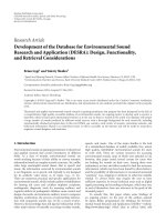
|z|=1. However, the forward difference method maps the
jω toacircleofradius0.5 and centered at the point z
= 0.5
as shown in Figure 1. Bilinear transform maps every point in
the jω-plane to the z-plane without aliasing.
We express ( 12)inmatrixformas
B
1
X

=

c
Δt

2
E
2
X,
(13)
where X

= [x

(0), x


(1), , x

(N − 1)]
T
, X =
[x(0), x(1), ,x(N −1)]
T
with
B
1
=
⎡
⎢
⎢
⎢
⎢
⎢
⎢
⎢
⎢
⎢
⎢
⎢
⎢
⎢
⎢
⎢
⎢
⎣

21 0 ··· 01
12 1
··· 0
01 2
.
.
.
.
.
.
.
.
.
.
.
.
.
.
.
.
.
.
.
.
.
.
.
.
.
.

.
.
.
.
1
10 0
··· 12
⎤
⎥
⎥
⎥
⎥
⎥
⎥
⎥
⎥
⎥
⎥
⎥
⎥
⎥
⎥
⎥
⎥
⎦
, (14)
E
2
=
⎡

⎢
⎢
⎢
⎢
⎢
⎢
⎢
⎢
⎢
⎢
⎢
⎢
⎢
⎢
⎢
⎢
⎣
−
21 0··· 01
1
−21··· 0
01
−2
.
.
.
.
.
.
.

.
.
.
.
.
.
.
.
.
.
.
.
.
.
.
.
.
.
.
.
.
.
.
1
100
··· 1 −2
⎤
⎥
⎥
⎥

⎥
⎥
⎥
⎥
⎥
⎥
⎥
⎥
⎥
⎥
⎥
⎥
⎥
⎦
. (15)
Hence, we conclude with an equivalent form of discrete
second derivative as
X

=

c
Δt

2
B
−1
1
E
2

X,
(16)
with the discrete second derivative operator D
2
=
(c/Δt)
2
B
−1
1
E
2
.
3. Obtaining DFT Commuting Matrices
An easy and accurate way of obtaining Hermite-Gaussian-
like eigenvectors of the DFT matrix is to define a better
commuting matrix, which imitates the Hermite-Gaussian
generating differential equation given in (3) as a discrete
substitute. In this section we disclose an elegant way of
obtaining better commuting matrices by taking advantage of
the bilinear transform, which is a good discrete substitute for
the derivative operator.
The algorithm is straightforward; we substitute the
second derivative and the Fourier transform operators in
(3) with the matrix given in (16) and the DFT matrix,
−1
−0.8
−0.6
−0.4
−0.2

0
0.2
0.4
0.6
0.8
1
−1 −0.8 −0.6 −0.4 −0.20 0.20.40.60.81
Real {z}
Figure 1: Image of jω axis in the z-plane for bilinear transform and
the forward difference method. Solid: bilinear transform, dashed:
forward difference method.
respectively. Hence, DFT commuting matrix inspired by the
bilinear transform is given by
B
= B
−1
1
E
2
+ FB
−1
1
E
2
F
−1
.
(17)
We omit the coefficient (c/Δt)
2

, since it has no effect on the
eigenvectors of B.
Theorem 2. B commutes with the DFT matrix.
Proof. As B
1
and E
2
are both circulant and symmetric, B
−1
1
E
2
is symmetric and circulant also. We use Theorem 1 given in
Section 2.2, which states that any circulant and symmetric
matrix C can be used to generate a commuting matrix as in
(10). Since B
−1
1
E
2
is both circulant and symmetric, the proof
is complete.
After generating the commuting matrix B, we find its
eigenvectors. The eigenvectors are Hermite-Gaussian-like
eigenvectors with the number of zero-crossings equal to the
order of Hermite-Gaussian eigenvectors. In Section 4 we give
extensive simulations and results on these Hermite-Gaussian
like eigenvectors.
3.1. Stability. Stability of B can easily be proved when
B

1
is not singular. We can show this by the eigenvalue
decomposition of B
1
B
1
= F
−1
Λ
B
1
F,
(18)
where Λ
B
1
is a diagonal matrix containing the eigenvalues
of B
1
.AsB
1
is circulant, the eigenvalues are Λ
B
1
=
diag(
√
NFb
1
), where b

1
is the first column of B
1
and N × N
4 EURASIP Journal on Advances in Signal Processing
is the dimension of Λ
B
1
.Asb
1
= [2,1,0,0, ,1]
T
,Fourier
transform of b
1
can be easily found and replaced to find the
eigenvalues Λ
B
1
Λ
B
1
= diag

2+2cos

2πn
N

, n = 0, 1, 2, , N −1.

(19)
Λ
B
1
is never zero for odd N, since diag(2 + 2 cos(2πn/N)) >
0foralln.HoweverasN increases Λ
B
1
becomes poorly
conditioned. Besides, for even N, diag(2+2 cos(2πn/N))
= 0
for n
= N/2, which causes instability. We can add a small
ξ>0 in the diagonal of B
1
to overcome instability. Then Λ
B
1
is changed to
Λ
B
1
= diag

2+ξ +2cos

2πn
N

, n = 0, 1, 2, , N −1

(20)
to preserve stability for even N. Consequently, to ensure
stability we substitute B
1
defined in (14)with

B
1
=
⎡
⎢
⎢
⎢
⎢
⎢
⎢
⎢
⎢
⎢
⎢
⎢
⎣
2+ξ 10··· 01
12+ξ 1
··· 0
012+ξ
.
.
.
.

.
.
.
.
.
.
.
.
.
.
.
.
.
.
.
.
.
.
.
.
.
.
.
.
.
.
1
100
··· 12+ξ
⎤

⎥
⎥
⎥
⎥
⎥
⎥
⎥
⎥
⎥
⎥
⎥
⎦
. (21)
Adding a small ξ value in the diagonal will not perturb the
eigenvectors of the commuting matrix.
3.2. Be tter Conditioned Bilinear Methods. Bilinear transform
can be considered as a trapezoidal approach to the derivative.
Hence, we can assure stability by using alternative B
1
matrices. We have found out that changing the diagonal
of B
1
by a constant k>2 both ensures the stability and
increases the performance. Therefore we substitute B
1
with
B
1
, where we define B
1

as
B
1
=
⎡
⎢
⎢
⎢
⎢
⎢
⎢
⎢
⎢
⎢
⎢
⎢
⎣
k 10··· 01
1 k 1
··· 0
01 k
.
.
.
.
.
.
.
.
.

.
.
.
.
.
.
.
.
.
.
.
.
.
.
.
.
.
.
.
.
.
1
10 0
··· 1 k
⎤
⎥
⎥
⎥
⎥
⎥

⎥
⎥
⎥
⎥
⎥
⎥
⎦
. (22)
As k>2, the commuting matrix is better conditioned. The
optimum value of k is found to be approximately 4.3, which
is given in Section 4.
3.3. Higher-order Bilinear Differentiation Matrix Substitutes.
So far, we have used the bilinear—transform—inspired
matrices to find a better discrete substitute for the sec-
ond derivative. To find better definitions of differentiation
matrices we suggest that a Taylor series-like approach to
B
1
Table 1: Optimum a
i
coefficients generated for B
14
.
a
i
Optimum Value
a
1
1.00
a

2
0.247634068038315
a
3
−0.103839534211561
a
4
−0.141176982675410
a
5
0.005956945393076
a
6
−0.008133047918379
a
7
−0.020103743248487
a
8
−0.001866823892062
a
9
−0.000336065416294
a
10
−0.002383849560258
a
11
−0.000725049220057
a

12
−0.000698349278537
a
13
−0.003339855815284
a
14
−0.001759635742928
(1) Compute one of

B
1
, B
1
,orB
n
matrices.
(2) Replace the computed matrix in (17)asasubstitutefor
B
1
and compute the DFT-commuting matrix B.
(3) Find the eigenvectors of B, which are Hermite-
Gaussian-like orthonormal vectors.
Algorithm 1: Summary of the proposed algorithms.
will grant us higher-order bilinear differentiation matrices.
Therefore, we define higher-order bilinear differentiation
matrices as
B
n
= a

1
B
1
+ a
2

B
1

2
+ ···+ a
n

B
1

n
, (23)
where we name
B
n
as nth-order bilinear approximation to
the second derivative, and a
i
arerealscalars.Thevalueofk =
4.3 is chosen for B
n
,asitisanoptimumvaluewithrespectto
minimum total error norm which is discussed in Section 4.
We have not come up with an analytical expression of a

i
’s
yet, however, genetic and/or pattern search algorithms may
be used to optimize the coefficients.
We have used the genetic [16] and the pattern search
[17] algorithms and determined optimum a
i
coefficients,
i
= 1, 2, , 14, which are given in Tabl e 1. These coefficients
are inserted in (23)toobtain
B
14
.Wehavegeneratedthe
commuting matrix B by substituting B
1
with B
14
in (17).
When
B
14
is employed, eigenvectors of B are found to be
very close to the samples of Hermite-Gaussian functions as
the performance is discussed in detail in the very Section 4.
So far, three different methods are proposed, which are
summarized in Algorithm 1. The first method computes

B
1

,inwhichasmallξ is added in the diagonal of B
1
to achieve stability. In the second method we alter the
diagonal of
B
1
,withavaluek>2. Changing the diagonal
both improves the performance and ensures stability. In
the last proposed method we find higher-order matrices,
using the
B
1
and its weighted powers with k = 4.3
for a better definition of the commuting matrix. After-
wards, we replace the computed

B
1
, B
1
,orB
n
with B
1
in (17). The obtained matrix B is the DFT-commuting
EURASIP Journal on Advances in Signal Processing 5
5
10
15
20

25
30
35
40
45
50
55
2345678910
(k)
Total norm of error
N = 64
N
= 56
N
= 48
N
= 40
N
= 32
(a)
10
−2
10
−1
10
0
0 5 10 15 20 25 30
Number of zero crossing
log
10

(norm of error)

B
1
, k = 2+ξ
B
1
, k = 3
B
1
, k = 4
B
1
, k = 4.3
(b)
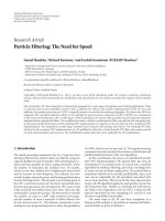
Figure 2: (a) The total norm of error versus k in B
1
for N = 32,
40, 48, 56, and k
= 4.3. The total norm of error is minimum when
k
≈ 4.3. (b) Error norms between the discrete Hermite-Gaussian
like eigenvectors and the samples of the Hermite-Gaussian
functions when
B
1
for k = 3, 4, and k = 4.3and

B
1

with N = 32.
matrix whose eigenvectors are the Hermite-Gaussian-like
orthonormal vectors.
4. Simulations and Results
We have proposed three different techniques for finding
Hermite-Gaussian-like eigenvectors of the DFT. In the first
method we employ

B
1
defined in (21). As a second method
we use
B
1
as defined in (22)fordifferent values of k. Finally,
we employ
B
n
given in (23). We replace each matrices in
(17)asasubstitutetoB
1
to generate commuting matrices B.
Afterwards, we find eigenvectors of these commuting matri-
ces and find the norm of error between samples of corre-
sponding Hermite-Gaussian functions and the eigenvectors.
First we compare total norms of errors between the
Hermite-Gaussian functions and the samples of Hermite-
Gaussian-like eigenvectors to determine optimum k for
B
1

.
We define the total norm of error as sum of norms of error for
each eigenvector. Figure 2(a) shows the total norm of error
10
−6
10
−5
10
−4
10
−3
10
−2
10
−1
10
0
0 5 10 15 20 25 30
Number of zero crossings
log
10
(norm of error)
B
1
S
2
S
6
S
16

(a)
10
−8
10
−7
10
−6
10
−5
10
−4
10
−3
10
−2
10
−1
10
0
0102030405060
Number of zero crossings
log
10
(norm of error)
B
1
S
2
S
6

S
16
(b)
Figure 3: Error norms between the discrete Hermite-Gaussian like
eigenvectors and the samples of the Hermite-Gaussian functions of
B
1
method when k = 4.3 are compared with various other methods
for (a) N
= 32 and (b) N = 64.
versus k for different values of N, and the best value for k is
approximately 4.3.
Comparison of errors between
B
1
for k = 3, 4, and 4.3
and

B
1
with the dimensional N = 32 is given in Figure 2(b).
The error norm is measured as the norm of error between
the samples of Hermite-Gaussian functions and Hermite-
Gaussian like eigenvectors of B using these matrices. As it
is clear from the figures, the best overall performance is
obtained in the
B
1
method when k = 4.3.
Figure 3(a) plots the norms of errors for different

methods defined in [8]. We compare the error norms of
S
2
, S
6
,andS
16
in between, which are of O(h
2
), O(h
6
), and
O(h
16
) Taylor approximations, respectively, as shown in [8],
with the
B
1
method, k = 4.3forN = 32. Figure 3(b) plots
6 EURASIP Journal on Advances in Signal Processing
0
0.2
0.4
0.6
0.8
1
1.2
1.4
0 5 10 15 20 25 30 35
Number of zero crossings

Norm of error
B
14
S
100
S
400
S
32
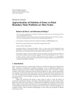
Figure 4: Comparison of error norms between the discrete
Hermite-Gaussian like eigenvectors and the samples of the
Hermite-Gaussian functions of
B
14
and S
32
, S
100
,andS
400
methods
for N
= 32.
the same comparison for N = 64. These plots show that
our proposed algorithm is slightly worse than some other
methods for small orders, but much better for higher-orders
of eigenvectors. As it is clear from the figures, our method
outperforms the other methods in total.
We compare the proposed higher-order
B

14
method
with the other higher-order methods, S
32
, S
100
,andS
400
that employ higher-order Taylor approximations to the
second derivative as shown in [10]. Figure 4 presents the
performance of the proposed method together with the other
methods. Despite the fact that our method uses only the
14th order approximation, it is definitely better than these
methods, even better than S
400
.
5. Conclusions
As the eigenvectors that are closer to the samples of
continuous Hermite-Gaussian functions are important for
a better definition of DFrFT, we employ bilinear transform-
based methods to define better commuting matrices. We
have proposed three different methods and analyzed their
stability issues. A stable method is proposed by inserting
asmallξ in the diagonal of the bilinear matrix. Better—
conditioned bilinear differentiation matrices that have
better performance are also obtained. Besides, a method of
generating higher-order bilinear differentiating matrices is
also suggested.
Simulation results show that the proposed methods
posess better eigenvectors when compared to the other

methods recently suggested.
Future works on this subject may include finding a
closed form expression for the coefficients generating the
higher-order bilinear matrices,
B
n
. Furthermore, B
n
matrices
may be used in linear combinations with other commuting
matrices, such as S
2k
.
References
[1]H.M.Ozaktas,Z.Zalevski,andM.A.Kutay,The Frac-
tional Fourier Transform with Applications in Optics and
Signal Processing, John Wiley & Sons, New York, NY, USA,
2001.
[2]M.A.Kutay,H.M.Ozaktas,O.Ankan,andL.Onural,
“Optimal filtering in fractional Fourier domains,” IEEE Trans-
actions on Signal Processing, vol. 45, no. 5, pp. 1129–1143,
1997.
[3] X G. Xia, “On bandlimited signals with fractional Fourier
transform,” IEEE Signal Processing Letters, vol. 3, no. 3, pp. 72–
74, 1996.
[4] O. Akay and G. F. Boudreaux-Bartels, “Fractional convolution
and correlation via operator methods and an application to
detection of linear FM signals,” IEEE Transactions on Signal
Processing, vol. 49, no. 5, pp. 979–993, 2001.
[5] B. Santhanam and J. H. McClellan, “The discrete rotational

Fourier transform,” IEEE Transactions on Signal Processing, vol.
44, no. 4, pp. 994–998, 1996.
[6] C¸ . Candan, M. A. Kutay, and H. M. Ozaktas, “The discrete
fractional Fourier transform,” IEEE Transactions on Signal
Processing, vol. 48, no. 5, pp. 1329–1337, 2000.
[7] S C. Pei, W L. Hsue, and J J. Ding, “Discrete fractional
Fourier transform based on new nearly tridiagonal commut-
ing matrices,” IEEE Transactions on Signal Processing, vol. 54,
no. 10, pp. 3815–3828, 2006.
[8] C¸ . Candan, “On higher order approximations for Hermite-
Gaussian functions and discrete fractional Fourier trans-
forms,” IEEE Signal Processing Letters, vol. 14, no. 10, pp. 699–
702, 2007.
[9] S C. Pei, J J. Ding, W L. Hsue, and K W. Chang, “Gener-
alized commuting matrices and their eigenvectors for DFTs,
offset DFTs, and other periodic operations,” IEEE Transac-
tionsonSignalProcessing, vol. 56, no. 8, pp. 3891–3904,
2008.
[10] S C. Pei, W L. Hsue, and J J. Ding, “DFT-commuting
matrix with arbitrary or infinite order second derivative
approximation,” IEEE Transactions on Signal Processing, vol.
57, no. 1, pp. 390–394, 2009.
[11] B. Santhanam and T. S. Santhanam, “Discrete Gauss-Hermite
functions and eigenvectors of the centered discrete Fourier
transform,” in Proceedings of the IEEE International Conference
on Acoustics, Speech and Signal Processing ( ICASSP ’07), vol. 3,
pp. 1385–1388, 2007.
[12] B. W. Dickinson and K. Steiglitz, “Eigenvectors and functions
of the discrete Fourier transform,” IEEE Transactions on
Acoustics, Speech, and Signal Processing, vol. 30, no. 1, pp. 25–

31, 1982.
[13] F. A. Gr
¨
unbaum, “The eigenvectors of the discrete Fourier
transform: a version of the Hermite functions,” Journal of
Mathematical Analysis and Applications, vol. 88, no. 2, pp. 355–
363, 1982.
[14] A. Serbes and L. Durak, “Efficient computation of DFT
commuting matrices by a closed–form infinite order approxi-
mation to the second differentiation matrix,” Signal Process.In
press.
[15] G. G. Golub and C. F. Van Load, Matrix Computations,The
Johns Hopkins University Press, London, UK, 3rd edition,
1993.
EURASIP Journal on Advances in Signal Processing 7
[16] D. E. Goldberg, Genetic Algorithms in Search, Optimzation
and Machine Learning, Addison-Wesley, Reading, Mass, USA,
1989.
[17] C. Audet and J. E. Dennis Jr., “Analysis of generalized pattern
searches,” SIAM Journal on Optimization,vol.13,no.3,pp.
889–903, 2003.