Báo cáo sinh học: " Research Article Time-Frequency Data Reduction for Event Related Potentials: Combining Principal Component Analysis and Matching Pursuit" pot

Hindawi Publishing Corporation
EURASIP Journal on Advances in Signal Processing
Volume 2010, Article ID 289571, 13 pages
doi:10.1155/2010/289571
Research Article
Time-Frequency Data Reduction for Event Related Potentials:
Combining Principal Component Analysis and Matching Pursuit
Selin Aviyente,
1
Edward M. Bernat,
2
Stephen M. Malone,
3
and William G. Iacono
3
1
Department of Electrical and Computer Engineering, Michigan State University East Lansing, MI 48824, USA
2
Department of Psychology, Florida State University, Tallahassee, FL 32306, USA
3
Department of Psychology, University of Minnesota, Minneapolis, MN 55455, USA
Correspondence should be addressed to Selin Aviyente,
Received 2 February 2010; Revised 30 March 2010; Accepted 5 May 2010
Academic Editor: Syed Ismail Shah
Copyright © 2010 Selin Aviyente et al. This is an open access article distributed under the Creative Commons Attribution License,
which permits unrestricted use, distribution, and reproduction in any medium, provided the original work is properly cited.
Joint time-frequency representations offer a rich representation of event related potentials (ERPs) that cannot be obtained through
individual time or frequency domain analysis. This representation, however, comes at the expense of increased data volume and
the difficulty of interpreting the resulting representations. Therefore, methods that can reduce the large amount of time-frequency
data to experimentally relevant components are essential. In this paper, we present a method that reduces the large volume of
ERP time-frequency data into a few significant time-frequency parameters. The proposed method is based on applying the widely

used matching pursuit (MP) approach, with a Gabor dictionary, to principal components extracted from the time-frequency
domain. The proposed PCA-Gabor decomposition is compared with other time-frequency data reduction methods such as the
time-frequency PCA approach alone and standard matching pursuit methods using a Gabor dictionary for both simulated and
biological data. The results show that the proposed PCA-Gabor approach performs better than either the PCA alone or the standard
MP data reduction methods, by using the smallest amount of ERP data variance to produce the strongest statistical separation
between experimental conditions.
1. Introduction
Event-related potential (ERP) signals measured at the scalp
are produced by partial synchronization of neuronal field
potentials across the cortex [1]. This synchronization medi-
ates the “top-down” and “bottom-up” communication both
within and between brain areas and has particular impor-
tance during the anticipation of and attention to stimuli
or events. Event related potentials (ERPs) are obtained by
averaging EEG signals recorded over multiple trials or epochs
time-locked to the particular stimulus. ERP signal analysis
has proven to be effective in assessing the brain’s current
functional state and reflect many pathological processes (e.g.,
[2–6]).
Typically, ERP analysis is performed in the time domain,
where the amplitudes and latencies of prominent peaks in
the averaged potentials are usually measured and correlated
with information processing mechanisms. However, this
conventional approach has two major shortcomings. First,
it is well-known that ERPs are transient and nonstationary
signals. Second, ERPs generally contain multiple overlapping
processes operating across different time and frequency
ranges. A primary approach to this problem has been
to utilize time-frequency signal representations to detect
transient activity and to disentangle overlapping processes.

Several methods exist to fulfill this goal including wavelet
and wavelet packet decomposition [7–11], sparse signal
representations using overcomplete dictionaries (such as
matching pursuit [12, 13] and basis pursuit [14]), Cohen’s
class of time-frequency distributions [15, 16], and the
recently introduced high resolution time-frequency distribu-
tions [17–20].
Wavelet transforms have been successfully applied to
the analysis of evoked potentials in a variety of studies
[4, 7, 21]. They have been shown to be advantageous over
the Fourier transform, since the time varying frequency
information can be observed. However, wavelets have well-
known limitations in terms of time-frequency resolution
2 EURASIP Journal on Advances in Signal Processing
tradeoff, that is, at high frequencies, the temporal resolution
is high whereas the frequency resolution is low and vice versa
for low frequencies. Sparse representations such as matching
pursuit and basis pursuit aim to find a “best” fit to the given
signal in terms of the elements of a redundant family of
functions, called the dictionary [12, 13]. The “best” fit to
the given signal is quantified through both the mean square
error between the representation and the actual signal and
the sparseness of the representation, that is, the number of
elements of the dictionary used in the representation should
be minimal. This approach has the advantage of offering a
fully quantitative description of the ERPs by parameterizing
the time-frequency plane at the expense of being compu-
tationally expensive. Cohen’s class of distributions provides
advantages over the other time-frequency representations in
that it accurately characterizes the physical time-frequency

properties of a signal, for example, energy and marginals,
and yields uniformly high resolution over the entire time-
frequency plane [15, 22]. Recently, time-frequency distribu-
tions with improved resolution and concentration around
the instantaneous frequency have been introduced such as
the reassigned time-frequency representations, higher order
polynomial distributions, and complex-lag distributions [17,
20, 23]. Although these methods improve the resolution of
the representations, they come at the expense of increased
computational complexity and in some cases losing some
of the desirable properties such as the marginals. Moreover,
these distributions have been shown to be the most effective
for polynomial phase signals whereas ERPs have been shown
to be well represented by damped sinusoids [24], thus the
improvement provided by these more complex distributions
would be minimal. For these reasons, in this paper we will
focus on the Cohen’s class of distributions, in particular the
Reduced Interference Distributions.
The high resolution provided by Cohen’s class of time-
frequency distributions come at the expense of increased
data. The application of these distributions to large sets of
ERP data has tended to rely on a time-frequency region
of interest (TF-ROI; region of interest on the TF surface)
to define activity for evaluation. Therefore, there is a
growing need for data reduction and feature extraction
methods for reducing the three dimensional time-frequency
surfaces of ERPs to a few parameters. The problem of
feature extraction and data reduction has been traditionally
addressed using parametric and nonparametric methods.
Parametric approaches include sparse representations using

overcomplete dictionaries [12–14, 25–28], extraction of
features from the time-frequency distributions such as the
energy in different frequency bands, computation of higher
order joint moments [29, 30], and entropy [31]. Non-
parametric data reduction methods, on the other hand,
include data-driven multivariate component analysis such
as the application of matrix factorization methods to time-
frequency distributions. These methods include the non-
negative matrix factorization (NMF) [32–34], singular value
decomposition (SVD) [35], independent component analy-
sis (ICA) [1, 36], and principal component analysis (PCA)
[37–40] to extract time-frequency features for classification
purposes or for reducing the time-frequency surfaces to
a few meaningful components. The application of the matrix
factorization approaches have been mostly limited to decom-
posing a single time-frequency matrix into significant time
and frequency components to reduce the dimensionality
and extract features for consequent classification [34, 39].
However, in ERP analysis there is a need for multivariate
processing, that is, it is important to extract components
that describe a collection of signals, such as those collected
over multiple channels or multiple subjects. The principal
component analysis of time-frequency vectors representing
multiple subjects described in [37, 41] addresses this issue
by extracting time-frequency principal components over
a collection of ERP waveforms. At this point, it is also
important to motivate the use of PCA over other data
factorization methods. PCA is a multivariate technique that
seeks to uncover latent variables responsible for patterns of
covariation in the data set and has been used widely for

time domain ERP data description and reduction [42, 43].
It is commonly applied to the covariance of the data matrix
and is thus similar to SVD in the extracted components.
PCA does not make any strong assumptions about the data,
unlike NMF which imposes nonnegativeness, with the only
assumption being that the observations are linear functions
of the extracted components which is a common assumption
in ERP analysis. ICA has been proposed as a promising
alternative to PCA for ERP data reduction [1, 36]. However,
recent comparisons of PCA with ICA for ERP data analysis
indicates that ICA suffers from the component ”splitting”
problem, that is, components that should not be separated
are split into multiple components, and that it is more
suitable for spatial decompositions rather than temporal
ones [44, 45]. Further, ICA has been most commonly applied
to time-domain ERP signal representations, and its use
with time-frequency ERP representations has not been well-
validated. For these reasons, in the current paper we use PCA
as the first step in our data reduction algorithm.
In this paper, we address the data extraction and reduc-
tion problem in the time-frequency plane by combining
parametric and nonparametric methods in a nonstationary
setting. The ultimate goal is to find time-frequency com-
ponents that are common to a large set of ERP data and
that can summarize the relevant activity in terms of a few
parameters. We introduce a new data reduction method
based on applying matching pursuit decomposition to the
time-frequency domain principal components to further
reduce the information from the principal components and
to fully quantify the time-frequency parameters of ERPs.

Since the principal components extracted from ERP time-
frequency surfaces are well-localized in time and frequency,
we propose quantifying them in terms of well-known
compact signals, Gabor logons (in this paper, “Gabor logons”
and “logons” will be used interchangeably), on the time-
frequency plane. Even though there are various choices for
the basis functions that can be used to decompose a given
signal, in this paper Gabor logons are chosen for representing
time-frequency structure of ERP signals for two major
reasons. First, it is known that these functions achieve the
lower bound of the uncertainty principle (time-bandwidth
product) and have been described as the “elementary signals”
EURASIP Journal on Advances in Signal Processing 3
on the time-frequency plane [22, 46]. Second, the parameters
of the Gabor logons are well-suited for identifying between
transient versus oscillatory brain activity as well as separating
between overlapping time-frequency events with varying
duration or frequency oscillation. They have been widely
used in time-frequency representation of ERP signals [47–
49], in particular EEG phenomena including sleep spindles
[13, 50] and epileptic seizures [51]. An algorithm similar to
matching pursuit is developed in the time-frequency plane to
determine the best set of logons that describe each ERP time-
frequency principal component [12]. Fitting Gabor logons
to the extracted principal components offers three potential
benefits. First, decomposing the principal components (PCs)
into a few logons would capture the major activity described
by that principal component while at the same time serve
as a tool of denoising, that is, removing the unwanted
noise or activity that may exist in the principal component.

Second, insofar as a single logon can characterize the primary
activity in the experimental manipulations for each principal
component, this would offer evidence that the principal
components approach is efficientatextractingcompact
time-frequency representations. Finally, the extracted logons
offer an important unit of analysis in their own right, in
that they are maximally compact by definition. The proposed
methods are compared to both parametric and nonpara-
metric data reduction methods in the time-frequency plane,
namely, the standard matching pursuit algorithm [12, 52]
and PCA in terms of efficiency, computational complexity
and the effectiveness in describing the experimental effects
in the data. To evaluate these methods, we employ both
biological [41] and simulated data [37], that have been
previously evaluated using the PCA on the time-frequency
plane approach.
The rest of this paper is organized as follows. Section 2
gives a brief review of time-frequency distributions and
various matching pursuit approaches. Section 3 introduces
the data reduction method proposed in this paper, com-
bining principal component analysis with matching pursuit
on the time-frequency plane. Section 4 details the data
analyzed in this paper and presents the results of applying the
proposed method to both simulated data and ERP signals.
A comparison with different time-frequency data reduction
methods is also given in this section. Finally, Section 5
concludes the paper and discusses the major contributions.
2. Background
2.1. Time-Frequency Distribut ions. A bilinear time-frequen-
cy distribution (TFD), C(t, ω), from Cohen’s class can be

expressed as (all integrals are from
−∞to ∞unless otherwise
stated) [22]
C
(
t, ω
)
=

φ
(
θ, τ
)
x

u +
τ
2

x
∗

u −
τ
2

×
e
j(θu−θt−τω)
dudθdτ,

(1)
where φ(θ, τ) is the kernel function in the ambiguity domain
(θ, τ), x(t) is the signal, and t and ω are the time and
the frequency variables, respectively. Some of the most
desired properties of TFDs are the energy preservation,
the marginals, and the reduced interference. For bilinear
time-frequency distributions, cross-terms occur when the
signal is multicomponent, that is, if x(t)
=

N
i=1
x
i
(t) then
C(t, ω)
=

N
i=1
C
x
i
,x
i
(t, ω)+

i
/
= j

2Re(C
x
i
,x
j
(t, ω)), where
C
x
i
,x
i
and C
x
i
,x
j
refer to the autoterms and cross-terms,
respectively. The cross-terms will introduce time-frequency
structures that do not correspond to the time-frequency
spectrum of the actual signal. For this reason, in this paper
we will use reduced interference distributions (RIDs) that
concentrate the energy across the autoterms, satisfy the
energy preservation and the marginals [53].
2.2. Matching Pursuit. The matching pursuit algorithm,
originally proposed by Mallat, aims at obtaining the “best”
linear representation of a signal in terms of functions,
{g
i
}
i=1,2, ,N

(sometimes referred to as atoms), from an over-
complete dictionary, D, using an iterative search algorithm
[12].
(1) Define the 0th order residual as R
0
x = x,

D = D and
set k
= 0.
(2) For the kth order residual, R
k
x, select the best atom
such that the inner product between the residual and
the atom is maximized
g
k
= argmax
g
i
∈

D




R
k
x, g

i




.
(2)
(3) Compute the residue R
k+1
x as
R
k+1
x = R
k
x −

R
k
x, g
k

g
k
. (3)
(4) Set k
= k +1,

D =

D \g

k
, and go back to step 2 until
a predetermined stopping criterion is achieved. The
stopping criterion can either be a preselected number
of atoms to describe the signal or a percentage
of energy of the original signal described by the
selected atoms. After M iterations, the following
linear representation is obtained:
x
=
M

k=1

R
k
x, g
k

g
k
+ R
M+1
x.
(4)
This procedure converges to x in the limit, that is, x
=

∞
k=1

R
k
x, g
k
g
k
, and preserves signal energy.
2.3. Simultaneous Matching Pursuit. The principle of MP
can easily be generalized to the simultaneous decomposition
of multiple signals, X
= (x
1
, x
2
, ,x
r
), into atoms from
the same overcomplete dictionary, D. This approach is
sometimes referred to as the multichannel matching pursuit
or the multivariate matching pursuit (MMP) algorithm
in literature since it is usually applied to multiple signals
collected over multiple channels or sensors [52, 54–56]. In
this paper, we will refer to this method as the simultaneous
matching pursuit (SMP) to avoid any confusions since the
4 EURASIP Journal on Advances in Signal Processing
method will be applied to multiple ERPs from different
subjects and not from multiple channels. This algorithm can
be described as follows.
(1) Define for each signal x
l

the 0th order residual as
R
0
x
l
= x
l
and set

D = D, k = 0.
(2) For the kth order residual, R
k
x
l
, select the best atom
such that the sum of the squared inner products
between the atom and the residual from each signal
is maximized
g
k
= argmax
g
i
∈

D
r

l=1





R
k
x
l
, g
i




2
.
(5)
(3) Compute the residue R
k+1
x
l
for each signal:
R
k+1
x
l
= R
k
x
l
−


R
k
x
l
, g
k

g
k
. (6)
(4) Set k
= k +1,

D =

D \g
k
, and go back to step 2 until
a predetermined stopping criterion is achieved. The
stopping criterion can either be a preselected number
of atoms to describe the collection of signals or an
average percentage of energy of the original signals
described by the selected atoms. After M iterations,
the following linear representation is obtained for
each signal:
x
l
=
M


k=1

R
k
x
l
, g
k

g
k
+ R
M+1
x
l
.
(7)
3. PCA-Gabor Method
Ideally, a time-frequency domain ERP data reduction
method will faithfully reproduce established time and
frequency-based findings (i.e., peaks in the time domain such
as P300 or summaries of frequency activity such as alpha),
and also allow a more complex view of these phenomena
using the joint time-frequency information available in the
TFDs. The decomposition method used in this paper is based
on two stages of consecutive data reduction. The first stage
is a direct extension of PCA into the joint time-frequency
domain and the second stage is the parametrization of
the time-frequency principal components using a matching

pursuit type algorithm.
3.1. PCA on the Time-Frequency Plane. The first stage of the
algorithm extends principal component analysis to the time-
frequency plane as follows.
(1) Compute the time-frequency distribution of each
ERP waveform from multiple subjects, x
i
,1≤ i ≤ L:
TFD
i

n, ω; ψ

=
N

n
1
=−N
N

n
2
=−N
x
i
(
n + n
1
)

x
∗
i
(
n + n
2
)
×ψ

−
n
1
+ n
2
2
, n
1
−n
2

e
−jω(n
1
−n
2
)
,
(8)
where ψ is the discrete-time kernel in the time and
time-lag domain and x

i
(n) is the ith ERP waveform.
In this paper, the binomial kernel, given by
ψ
(
n, m
)
= 2
−|m|
⎛
⎝
|
m|
n +
|m|
2
⎞
⎠
for |n|≤
|
m|
2
,(9)
is used as the time-frequency kernel.
(2) Given L ERPwaveforms,rearrangethetime-
frequency surfaces into vectors and form the matrix
X
=
⎡
⎢

⎢
⎢
⎢
⎢
⎣
TFD
T
1
TFD
T
2
.
.
.
TFD
T
L
⎤
⎥
⎥
⎥
⎥
⎥
⎦
. (10)
(3) Compute the covariance matrix, Σ
= XX
T
.
(4) Decompose the covariance matrix using principal

component analysis
Σ
=
L

j=1
λ
j
PC
j
PC
T
j
,
(11)
where λ
j
is the eigenvalue of each principal compo-
nent PC
j
. The principal components determine the
span of the time-frequency space.
(5) Rotate the principal components using varimax
rotation [57]. Varimax rotation is an orthogonal
transform that rotates the principal components such
that the variance of the factors is maximized. This
rotation improves the interpretability of the principal
components.
(6) Rearrange each principal component into a time-
frequency surface to obtain the ERP components in

the time-frequency domain.
After the principal components on the time-frequency plane
are extracted, they are ordered based on their eigenvalues
and the most significant ones are used in the following
parametrization stage. The number of principal components
to keep is determined based on a normalized energy
threshold.
3.2. Matching Pursuit on the Time-Frequency Plane. In this
section, we introduce a matching pursuit type algorithm in
the time-frequency domain to further parameterize the ERP
time-frequency surfaces. The goal is to be able to describe
the principal components using a compact set of time-
frequency parameters using Gabor logons as the dictionary
elements. The proposed algorithm is similar to the original
matching pursuit [12] and the discrete Gabor decomposition
[58], except that it is directly implemented in the time-
frequency domain rather than in the time domain. This
implementation is preferred over the standard MP for two
reasons. First, the principal components are already in the
time-frequency domain, and inverting them back to the
EURASIP Journal on Advances in Signal Processing 5
time domain would increase the computational complexity.
Second, this offers a way of directly modeling the time-
frequency energy distribution.
An overcomplete dictionary of Gabor logons on the
time-frequency plane is constructed by computing the time-
frequency distribution of discrete time atoms g(n; n
0
, k
0

) =
exp(−(1/2σ
2
)(n − n
0
)
2
)exp(j2π(k
0
/K)(n − n
0
)) where σ
is the scale parameter, n
0
and k
0
are the discrete time
and frequency shift parameters, respectively, and K is the
total number of frequency samples. The elements of the
dictionary, D, are the binomial TFDs of these atoms, G
i
(n, k).
The number of elements in the dictionary are determined
by the range of n
0
, k
0
and σ. In this paper, n
0
= 1, , N,

where N is the total number of time samples, k
0
= 1, , K,
where K is the total number of frequency samples, and σ
=
{
1, 2, 4, ,2
log
2
N−1
}.
The proposed greedy search algorithm is an extension of
the orthogonal matching pursuit (OMP) described in [59]
to the time-frequency domain. The orthogonal matching
pursuit adds a least-squares minimization to each step of MP
to obtain the best approximation over the atoms that have
already been chosen. This revision significantly improves
the convergence speed of the algorithm. For a given time-
frequency matrix, TFD, the search for logons that best
describe the surface can be summarized as follows.
(1) Initialize the residue as R
0
= TFD and set l = 0and

D = D.
(2) At the lth iteration, find the Gabor logon over
the whole overcomplete dictionary, that is, over all
(n
0
, k

0
, σ), that has the largest inner product with the
residue time-frequency surface, R
l
G
l
(
n, k
)
= argmax
G
i
(
n,k
)
∈

D




R
l
, G
i





=
argmax
G
i
(
n,k
)
∈

D






N

n=1
K

k=1
R
l
(
n, k
)
G
i
(

n, k
)






.
(12)
(3) Compute the approximation at the lth step, A
l
,as
A
l
= argmin
A
TFD −A
2
,
(13)
where A
∈ span{G
i
, i = 1,2, , l}.Thisproblemis
solved using a least squares optimization approach.
(4) Subtract the approximation, A
l
, from the residue to
compute the new residue time-frequency distribu-

tion at the l + 1th iteration
R
l+1
(
n, k
)
= R
l
(
n, k
)
−A
l
(
n, k
)
.
(14)
(5) Increment l by 1, set

D =

D \G
l
.
(6)Gobacktostep2untilapredeterminednumberof
atoms is selected or the normalized mean squared
error (NMSE) between the TFD and the approxi-
mation at the lth iteration is below a predetermined
threshold, that is,

NMSE
=



TFD −A
l



2
2
TFD
2
2
=

N
n=1

K
k=1

TFD(n, k) −A
l
(
n, k
)

2


N
n
=1

K
k
=1
TFD
2
(
n, k
)
<γ.
(15)
NMSE is a measure of how close the approximation
from the dictionary is to the original time-frequency
distribution. Since the mean square error is normal-
ized by the energy of the original TFD, it is always
between 0 and 1.
4. Simulated and Biological Data Analysis
4.1. Description of Biological D ata. The biological data used
in this paper has been previously presented utilizing PCA
on the time-frequency plane approach, and thus we will
only detail the relevant parameters here. The reader is
directed to the previously published paper for greater detail
[41]. The sample consisted of twins in the Minnesota Twin
Family Study (MTFS), a longitudinal and epidemiological
investigation of the origins and development of substance use
disorders and related psychopathology. All male and female

twin participants for whom ERP data were available from the
study’s psychophysiological assessment served as subjects for
this investigation. This sample combined subjects from the
two age cohorts of the MTFS. Subjects in one cohort were
17 years old at intake whereas subjects in the other were
approximately 11 years old at intake. Data for this younger
cohort came from a follow-up assessment conducted when
subjects were approximately 17 years old. The sample thus
comprised 2,068 17-year-old adolescents in all (mean age
=
17.7; SD = 0.5; range = 16.7 to 20.0).
A visual oddball task was used. Each of the 240 stimuli
comprising this task was presented on a computer screen
for 98 ms, with the intertrial interval (ITI) varying randomly
between 1 and 2 s. A small dot, upon which subjects were
instructed to fixate, appeared in the center of the screen
during the ITI. On twothirds of the trials, participants saw a
plain oval to which they were instructed not to respond. On
the remaining third of the trials, participants saw a superior
view of a stylized head, depicting the nose and one ear. These
stylized heads served as “target” stimuli. Participants were
instructed to press one of two response buttons attached to
each arm of their chair to indicate whether the ear was on
the left side of the head or the right. Half of these target trials
consisted of heads with the nose pointed up, such that the
left ear would be on the left side of the head as it appeared
to the subject (easy discrimination). Half consisted of heads
rotated 180 degrees so that the nose pointed down, such that
the left ear would appear on the right side of the screen and
the right ear would appear on the left side of the ear (hard

discrimination).
6 EURASIP Journal on Advances in Signal Processing
For each trial, 2 s of EEG, including a 500 ms prestimulus
baseline, were collected at a sampling rate of 256 Hz. EEG
data were recorded from three parietal scalp locations, one
on the midline (Pz) and one over each hemisphere (P3 and
P4). Consistent with the previous report, only data from
the Pz electrode is reported here. Similarly, although ERPs
to standard (frequent) stimuli were collected, they were not
analyzed for the current paper; target condition responses
serve as the basis for all decompositions and analyses
presented. Therefore, the analysis in this paper focuses on
data reduction for ERPs collected across multiple subjects
from a single channel. However, the methods developed can
easily be extended to single subject and/or multiple channel
data.
Principal component decompositions were employed
to evaluate the proposed approach. For the purposes of
this study, decompositions for condition-averaged data were
conducted on narrow time and frequency ranges, to focus
on lower frequency delta and theta activity. Condition-
averaged ERPs were constructed separately for easy and
hard discrimination conditions. These included frequencies
ranging from 0 to 5.75 Hz and time ranging from stimulus
onset to 1000 ms poststimulus. The range was narrowed to
focus on the time-frequency range containing the majority
of variance: theta, delta, and low frequency activity.
4.2. Description of Simulated Data. Two simulated datasets
were employed in the current paper. As with the biological
data, these datasets were employed previously with PCA

approach alone [37]. Briefly, the two sets included are 3-
logons and 3-logons with noise. All simulated sets were
100 Hz sampled signals of 1000 ms, with the first and last
100 ms discarded after the TFD is computed to remove edge
effects. The first simulated dataset contains 3 logons with
clearly separated time and frequency centers: 30 Hz/100 ms,
20 Hz/400 ms, and 10 Hz/700 ms. For 3-logons with noise,
noise was added at the 4 dB signal to noise level. In all
simulations, each signal entered was assigned to a different
simulated topographical region, to simulate the activity from
different brain areas. To accomplish this, the signals were
divided into 63 simulated channels creating a 7
× 9grid
within which differential weightings could be applied. Each
signal entered, that is, each logon, was weighted by a 4
× 4
grid differentially located within the overall 7
× 9 grid. The
differential loadings were implemented to simulate a signal
with more focal activity that decays in topographic space.
The simulated datasets each contained 7560 total waveforms,
comprised of 120 trials by 63 electrodes.
4.3. Results. In this section, we will present the results of
applying the PCA-Gabor method on both simulated data and
ERP signals described above. In the PCA-Gabor analysis, we
will focus on extracting the “best” logon fit to the principal
component surface. Extracting the “best” logon offers a way
of parameterizing the PCs using the time, frequency and scale
parameters of the logon as well as serving as a denoising tool
since the “best” logon will focus on representing the actual

signal energy as opposed to background noise. Through
Table 1: The comparison of the variance explained by the PCA,
PCA-Gabor, and SMP-Gabor for two simulated datsets: 3-logons
and 3-logons in noise.
Data Set PCA PCA-Gabor SMP-Gabor
3 Logons 99.97% 95.73% 95.73%
3 Logons in Noise 81.38% 90.78% 38.20%
this analysis, we will show the effectiveness of the PCA-
Gabor method both as a modeling/data reduction tool
and a denoising tool. The proposed method also offers an
alternative to previous ERP studies that use matching pursuit
to decompose each signal individually [13]. This analysis
has the disadvantage of being computationally expensive and
extracting a large number of logons to represent a collection
of signals. Since a comparison between matching pursuit at
the individual signal level and the PCA-Gabor method would
not be helpful due the number of logons extracted being
much larger for the MP, we compare the PCA-Gabor method
to the simultaneous matching pursuit with Gabor dictionary
(SMP-Gabor) and to previous results obtained by the PCA
method on the time-frequency plane [37].
4.3.1. Analysis of Simulated Data. The different methods
were first evaluated for simulated data made up of Gabor
logons. For this analysis, decompositions from two simulated
datasets containing 3-logons with and without additive white
noise were used. The PCA approach involved selecting the
three time-frequency PCs with the highest eigenvalues. The
PCA-Gabor approach extracted the “best” Gabor logon for
each of the three PCs yielding three logons. Finally, the SMP-
Gabor method extracted the best three logons that explained

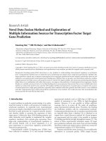
the whole data set. For the 3-logons without noise all of
the methods explained more than 95% variance of the data
set with the PCA performing the best (Table 1). The logons
extracted from PCA-Gabor and SMP-Gabor were identical
(see Figure 1) explaining exactly the same amount of data
variance indicating that under ideal conditions PCA-Gabor
performs as well as the standard SMP-Gabor.
For 3-logons in 4 dB noise, similarly, three components
were extracted by each of the algorithms, that is, three PCs
with PCA, three logons fitted to the PCs with PCA-Gabor,
and three logons fitted to the whole dataset with SMP-Gabor.
The extracted components were evaluated in terms of the
amount of signal variance they captured by projecting the
components onto the original 3-logon dataset. From Tabl e 1,
it can be seen that PCA-Gabor captures the most amount
of signal variance with PCA coming in second. The logons
extracted from the SMP-Gabor method can only explain
38.20% of the total signal variance since the algorithm
focuses on extracting components that capture the most
amount of common variance in the data (whereas PCA is
covariance-based), which in this case corresponds to noise.
Figure 1 illustrates how the logons extracted by SMP-Gabor
become wider in time and less correlated with the actual
logons for the noisy data. This figure also shows that PCA-
Gabor acts as a denoising mechanism reducing the noise in
the PCs and thus representing more of the signal.
EURASIP Journal on Advances in Signal Processing 7
Grand average
No noise
(Hz)

0
20
40
(ms)
0 400 800
With noise
(Hz)
0
20
40
(ms)
0 400 800
TF
amplitude
High
Low
(a)
Decomposition
No noise With noise
PCA PCA-gabor SMP-gabor PCA PCA-gabor SMP-gabor
(Hz)
0
20
40
(Hz)
0
20
40
(Hz)
0

20
40
Components
(ms)
04 8
×10
2
(ms)
04 8
×10
2
(ms)
048
×10
2
(ms)
04 8
×10
2
(ms)
04 8
×10
2
(ms)
04 8
×10
2
TF
amplitude
High

Low
(b)
Figure 1: A comparison of the principal components (PCA), Gabor logons extracted from the principal components (PCA-Gabor) and
Gabor logons extracted by Simultaneous Matching Pursuit using a Gabor dictionary (SMP-Gabor) from two simulated datasets (3-logons
with no noise and 3-logons with noise).
Table 2: Partial eta-squared (η
2
p
) values from a repeated-measures
general linear model (GLM) for the three methods for ERP analysis.
Multivariate tests indicate statistical values across all components.
Note:
∗
P<.05,
∗∗
P<.01, and
∗
P<.001.
Factors Sex RT Difficulty
Multivariate PCA .102
∗∗∗
.105
∗∗∗
.088
∗∗∗
Multivariate PCA-Gabor .105
∗∗∗
.109
∗∗∗
.091

∗∗∗
Multivariate SMP-Gabor .086
∗∗∗
.104
∗∗∗
.084
∗∗∗
4.3.2. Analysis of Biological Data. For the biological data,
first we will compare the variance characterized using the
different approaches. We extract 11 PCs using PCA, the 11
logons extracted from these PCs using PCA-Gabor, and 11
logons that best explain the energy of the whole dataset using
the SMP-Gabor method. Once the different components
are extracted, they are projected onto each of the 8328
condition-averaged ERP waveforms. For the three methods
compared in this paper, PCA, PCA-Gabor and SMP-Gabor,
PCA explained most of the data variance with 91%. For SMP-
Gabor, the variance explained was 81% whereas for PCA-
Gabor it was 70%.
While the PCA explains the most overall variance in
the data, and PCA-Gabor the least, additional analysis is
needed to evaluate the methods in terms of experimentally
relevant variance. To accomplish this, the three methods
were compared for statistical separation using three common
variables: sex, reaction time, and task difficulty. Because the
activity extracted from the three methods covers much of
the same time-frequency range, it is expected that the three
methods should provide similar statistical effects. Statistical
evaluation was conducted using a repeated-measures general
linear model (GLM) including sex, reaction time, and task

difficulty. A separate GLM was conducted for the sets of
11 components from each method. The design was Sex
(male/female) by RT (reaction time; continuous) by task
Difficulty (easy/hard; the within-subjects repeated measure).
These main effects were highly significant for all three
methods, confirming that similar experimentally relevant
activity was extracted. Partial eta-squared (η
2
p
)valuesfor
the three methods are summarized in Table 2.Here,for
sex, RT, and difficulty, the nominal order of the amount of
experimentally relevant variance in the statistical effects was
the same, largest in the PCA-Gabor, next in the PCA, and the
least in the SMP-Gabor.
By comparing the data reduction methods in terms of
both overall data variance as well as experimentally relevant
variance, stronger inferences can be made about how well
the methods perform. In particular, the PCA-Gabor method
captured the largest amount of experimentally relevant vari-
ance, while using the least amount of overall data variance.
8 EURASIP Journal on Advances in Signal Processing
Table 3: A qualitative comparison of the three data reduction methods discussed in this paper.
Method/Properties Data dependent
Time-Frequency
Parametrization
Computation time Variance versus Covariance
PCA Yes
No
3.2 sec Covariance

PCA-Gabor Yes
Ye s
11.6 sec Covariance
SMP-Gabor No
Ye s
1276 sec Variance
Grand average
Microvolts
0
10
20
0 200 400 600 800 1000
(Hz)
0
2
4
TF
amplitude
0.3
0
(a)
Decomposition
PCA PCA-gabor SMP-gabor
(Hz)
0
2
4
(Hz)
0
2

4
(Hz)
0
2
4
(Hz)
0
2
4
(Hz)
0
2
4
(Hz)
0
2
4
(Hz)
0
2
4
(Hz)
0
2
4
(Hz)
0
2
4
(Hz)

0
2
4
(Hz)
0
2
4
Component 1
Component 11
(ms)
01
×10
3
(ms)
01
×10
3
(ms)
01
×10
3
TF
amplitude
0.3
0
(b)
Figure 2: A comparison of the principal components analysis (PCA), Gabor logons extracted from the principal components (PCA-Gabor),
and Gabor logons extracted by Simultaneous Matching Pursuit using a Gabor dictionary (SMP-Gabor) for the ERP dataset.
EURASIP Journal on Advances in Signal Processing 9
Grand average

Microvolts
0
10
20
0 200 400 600 800 1000
(Hz)
0
2
4
TF
amplitude
0.3
0
(a)
Decomposition
MP-grand average
(Hz)
0
2
4
(Hz)
0
2
4
(Hz)
0
2
4
(Hz)
0

2
4
(Hz)
0
2
4
(Hz)
0
2
4
(Hz)
0
2
4
(Hz)
0
2
4
(Hz)
0
2
4
(Hz)
0
2
4
(Hz)
0
2
4

Component 1
Component 11
(ms)
01
×10
3
TF
amplitude
0.3
0
(b)
Figure 3: 11 Gabor logons extracted from the grand average of ERP signals.
This is analogous to the results of the simulated data with
noise, where the PCA-Gabor method extracted the most
signal power in terms of experimentally relevant variance,
while excluding the largest amount of noise power in terms of
experimentally irrelevant variance. Thus, in these terms, the
PCA-Gabor method was the most optimal among the three
methods.
Finally, it is important to compare the different ap-
proaches in terms of computational complexity. All of the
algorithms are run on a PC with Pentium 4 processor at
2 GHz using MATLAB 7.0, and evaluated after generating the
time-frequency surfaces. The PCA-Gabor method took 11.6
seconds including the time to find the principal components
(3.2 seconds) and to search for the best logon fit for the
resulting PCs (8.4 seconds). The simultaneous matching
pursuit on the other hand took 1276 seconds. Thus, in
terms of computational complexity, PCA approach was the
fastest, followed closely by the PCA-Gabor method. Trailing

10 EURASIP Journal on Advances in Signal Processing
Table 4: The parameters (time center (samples), n
0
, frequency center (Hz), f
0
, and scale parameter σ) of the 11 logons extracted by PCA-
Gabor from the 11 PCs, SMP-Gabor from the 8238 TFD surfaces, and MP-Gabor from the grand average of the 8238 time-frequency surfaces.
PCA-Gabor SMP-Gabor Grand average-Gabor
Logon number n
0
f
0
σn
0
f
0
σn
0
f
0
σ
1 6 4.3128 1 15 1.265 8 15 1.265 8
2 7 1.4376 4 12 1.9837 8 12 1.955 8
3 16 0.9584 8 19 0.7188 16 19 0.7188 16
4 11 2.8752 1 12 2.7312 2 12 2.875 8
5 13 3.5940 1 27 1.4375 8 29 1.2363 4
6 5 3.3544 1 10 1.61 4 9 1.4375 4
7 14 2.1564 2 8 2.53 2 6 4.1113 1
8 8 2.3960 2 15 2.7025 1 12 4.1113 1
9 27 1.4376 8 19 1.9837 2 14 0.3738 8

10 23 1.9168 2 6 3.7950 1 19 2.3288 2
11 19 1.4376 4 9 3.5938 1 3 1.9837 4
by a large margin is the SMP-Gabor method, which was
computationally expensive due to the core search algorithm
required.
Ta ble 3 summarizes the key properties of the three
methods compared in this section in terms of their data
dependence, time and frequency parametrization, compu-
tational efficiency for the ERP data set and whether the
resulting decomposition is based on explaining the most
variance or covariance in the data.
4.4. Discussions. Several overall trends in the results are
important to detail. First, the PCA-Gabor characterized more
experimental variance than the PCA, with less of the overall
raw data variance. This suggests that the Gabor decom-
position of the PCA represents the relevant information
obtained in the PCA, supporting the view that the activity
extracted by PCA largely contains activity that conforms
to Gabor constraints. Second, because the PCA-Gabor
explains nominally more experimentally relevant variance,
and outperforms the SMP-Gabor, while using less of the raw
data variance than either, it supports the contention that this
approach produces a more optimal Gabor decomposition
of the collection of signals than the standard matching
pursuit. Finally, it is interesting to specifically consider the
fact that the PCA-Gabor method explains the least amount
of data variance compared to the other two methods. The
components extracted by PCA explain most of the data
variance since PCA is designed to maximize the variance
explained and extracts components that are orthogonal to

each other. The PCA-Gabor method, on the other hand,
approximates the energy of each principal component with
a single logon and thus, the total variance explained is
lower than the original principal components. However, this
method has the advantage of retaining the signal variance
and getting rid of the noise variance, thus acting as an
effective denoising method, while also parameterizing the
time-frequency surfaces. The third method, SMP-Gabor,
explains more of the data variance compared to PCA-
Gabor but has less experimental condition sensitivity (e.g.,
statistical significance). This increased variance and reduced
sensitivity can be explained by looking at the Gabor logons
extracted from the biological data by PCA-Gabor and
SMP-Gabor methods shown in Figure 1. Although the two
methods extract some common logons, SMP-Gabor method
emphasizes the low frequency activity. The first three logons
extracted by this method are low frequency logons with a
large time spread. The major reason for this is that the
SMP-Gabor method operates entirely on the variance, and
thus focuses the most on the high-amplitude (i.e., variance)
low-frequency area of the surface. The PCA approaches,
on the other hand, operate on covariance, which focuses
more on activity that is functionally related (i.e., covaries).
This point is also supported by the Gabor decomposition
of the grand average of the 8328 waveforms given in
Figure 3. Table 4 compares the parameters of the 11 logons
extracted from the 11 PCs using the PCA-Gabor method,
from the 8238 TFD surfaces using the SMP-Gabor method
and from the grand average of the 8238 waveforms using
standard MP-Gabor. This table indicates that there are some

commonalities between the SMP-Gabor and MP-Gabor on
the grand average surface since they extract similar logons
describing the low frequency activity, for example, logons 1-
3 are almost identical.
5. Conclusions
In this paper, a time-frequency data reduction method
combining a nonparametric data-driven approach, principal
component analysis, with a parametric approach, matching
pursuit with a Gabor dictionary, was presented. Using the
proposed method, it was possible to characterize large
amounts of ERP data with a small number of time-
frequency parameters. This joint application of PCA with
Gabor decomposition offered several advantages over indi-
vidual PCA and Gabor decomposition. First, compared
to PCA the proposed method improves the SNR of the
extracted components, that is, performs denoising, while
simultaneously parameterizing the time-frequency surfaces
and offering a succinct representation of the data set.
Second, the application of Gabor decomposition onto
EURASIP Journal on Advances in Signal Processing 11
the principal components instead of the actual data helps
to extract parameters that represent the covariation among
observations rather than characterize the average energy
across observations. This property of PCA-Gabor becomes
especially important when there is considerable noise in
the data since standard matching pursuit algorithms will
focus on fitting parameters to capture the most amount of
energy, which in this case may be noise components. This
phenomenon exhibited itself in the analysis of the biological
data as PCA-Gabor most effectively differentiated between

the experimental conditions with the least amount of data
variance, or in other words capturing the least amount of
noise, compared to the other two methods. This was mainly
because the extracted logons explained the main effects
described by the principal components with higher signal-
to-noise ratio (most experimentally relevant variance).
Future work will focus on the extensions of the proposed
methods to different data factorization approaches such as
the ICA. For ERP data collected over multiple channels,
spatial ICA may be used as an alternative to PCA and the
proposed data reduction method can be applied onto the
independent components. Future work will also evaluate the
Gabor parameters in relation to well-known cognitive ERP
events such as P300, as well as ERP events with known
specific neurological origins, such as anterior cingulate
cortex activation as measured in the error-related negativity
(ERN) paradigm.
Acknowledgments
This work was in part supported by Grants from the National
Science Foundation under CAREER CCF-0746971, National
Institutes of Health NIDA13240, NIDA05147, NIDA024417,
NIAA09367, and K08MH080239.
References
[1] S. Makeig, S. Debener, J. Onton, and A. Delorme, “Mining
event-related brain dynamics,” Trends in Cognitive Sciences,
vol. 8, no. 5, pp. 204–210, 2004.
[2] H. Shevrin, J. A. Bond, L. A. Brakel, R. K. Hertel, and W.
J. Williams, Conscious and Unconscious Processes: Psychody-
namic, Cognitive and Neurophysiological Convergences, Guil-
ford Press, New York, NY, USA, 1996.

[3] H.Shevrin,W.J.Williams,R.E.Marshall,R.K.Hertel,J.A.
Bond, and L. A. Brakel, “Event-related potential indicators of
the dynamic unconscious,” Consciousness and Cognition, vol.
1, no. 3, pp. 340–366, 1992.
[4] E. Bas¸ar, EEG-Brain Dynamics, Elsevier, Amsterdam, The
Netherlands, 1980.
[5] R. J. Sclabassi, M. Sun, D. N. Krieger, P. Jasiukaitis, and M.
S. Scher, “Time-frequency domain problems in the neuro-
sciences,” in Time-Frequency Signal Analysis: Methods and
Applications, B. Boashash, Ed., pp. 498–519, Longman, Har-
low, UK, 1992.
[6] W. J. Williams, H. P. Zaveri, and J. C. Sackellares, “Time-
frequency analysis of electrophysiology signals in epilepsy,”
IEEE Engineering in Medicine and Biology, vol. 14, no. 2, pp.
133–143, 1995.
[7] T. Demiralp, J. Yordanova, V. Kolev, A. Ademoglu, M. Devrim,
and V. J. Samar, “Time-frequency analysis of single-sweep
event-related potentials by means of fast wavelet transform,”
Brain and Language, vol. 66, no. 1, pp. 129–145, 1999.
[8] J. Raz, L. Dickerson, and B. Turetsky, “A wavelet packet model
of evoked potentials,” Brain and Language,vol.66,no.1,pp.
61–88, 1999.
[9] V. J. Samar, M. R. Raghuveer, K. P. Swartz, S. Rosenberg,
and T. Chaiyaboonthanit, “Wavelet decomposition of event
related potentials: toward the definition of biologically natural
components,” in Proceedings of the 6th IEEE Conference on
Statistical Signal and Array Processing, pp. 38–41, 1992.
[10] C. S. Herrmann, M. Grigutsch, and N. A. Busch, EEG
Oscillations and Wavelet Analysis, MIT Press, Cambridge,
Mass, USA, 2005.

[11] S. D. Cranstoun, H. C. Ombao, R. Von Sachs, W. Guo, and
B. Litt, “Time-frequency spectral estimation of multichannel
EEG using the auto-SLEX method,” IEEE Transactions on
Biomedical Engineering, vol. 49, no. 9, pp. 988–996, 2002.
[12] S. G. Mallat and Z. Zhang, “Matching pursuits with time-
frequency dictionaries,” IEEE Transactions on Signal Process-
ing, vol. 41, no. 12, pp. 3397–3415, 1993.
[13] P. J. Durka and K. J. Blinowska, “A unified time-frequency
parametrization of EEGs,” IEEE Engineering in Medicine and
Biology, vol. 20, no. 5, pp. 47–53, 2001.
[14] S. S. Chen, D. L. Donoho, and M. A. Saunders, “Atomic
decomposition by basis pursuit,” SIAM Journal of Scientific
Computing, vol. 20, no. 1, pp. 33–61, 1999.
[15] W. J. Williams, “Reduced interference distributions: biological
applications and interpretations,” Proceedings of the IEEE, vol.
84, no. 9, pp. 1264–1280, 1996.
[16] S. Haykin, R. J. Racine, X. U. Yan, and C. A. Chapman,
“Monitoring neuronal oscillations and signal transmission
between cortical regions using time-frequency analysis of
electroencephalographic activity,” Proceedings of the IEEE, vol.
84, no. 9, pp. 1295–1301, 1996.
[17] I. Shafi, J. Ahmad, S. I. Shah, and F. M. Kashif, “Techniques
to obtain good resolution and concentrated time-frequency
distributions: a review,” EURASIP Journal on Advances in
Signal Processing, vol. 2009, Article ID 673539, 43 pages, 2009.
[18]I.Shafi,J.Ahmad,S.I.Shah,andF.M.Kashif,“Computing
deblurred time-frequency distributions using artificial neural
networks,” Circuits, Systems, and Signal Processing, vol. 27, no.
3, pp. 277–294, 2008.
[19] I. Shafi, J. Ahmad, S. I. Shah, and F. M. Kashif, “Evolutionary

time-frequency distributions using Bayesian regularised neu-
ral network model,” IET Signal Processing,vol.1,no.2,pp.
97–106, 2007.
[20] I. Orovi
´
c and S. Stankovi
´
c, “A class of highly concentrated
time-frequency distributions based on the ambiguity domain
representation and complex-lag moment,” EURASIP Journal
on Advances in Signal Processing, vol. 2009, Article ID 935314,
9 pages, 2009.
[21] T. Demiralp, A. Ademoglu, M. Comerchero, and J. Polich,
“Wavelet analysis of P3a and P3b,” Brain Topography, vol. 13,
no. 4, pp. 251–267, 2001.
[22] L. Cohen, Time-Frequency Analysis, Prentice Hall, Upper
Saddle River, NJ, USA, 1995.
[23] M. Jachan, G. Matz, and F. Hlawatsch, “Time-frequency
ARMA models and parameter estimators for underspread
nonstationary random processes,” IEEE Transactions on Signal
Processing, vol. 55, no. 9, pp. 4366–4381, 2007.
12 EURASIP Journal on Advances in Signal Processing
[24] T. Demiralp, A. Ademoglu, Y. Istefanopulos, and H.
¨
O. G
¨
ulc¸
¨
ur,
“Analysis of event-related potentials (ERP) by damped sinu-

soids,” Biological Cybernetics, vol. 78, no. 6, pp. 487–493, 1998.
[25] J. A. Tropp, “Greed is good: algorithmic results for sparse
approximation,” IEEE Transactions on Information Theory, vol.
50, no. 10, pp. 2231–2242, 2004.
[26] R. Gribonval, “Fast matching pursuit with a multiscale
dictionary of Gaussian chirps,” IEEE Transactions on Signal
Processing, vol. 49, no. 5, pp. 994–1001, 2001.
[27] D. L. Donoho and X. Huo, “Uncertainty principles and ideal
atomic decomposition,” IEEE Transactions on Information
Theory, vol. 47, no. 7, pp. 2845–2862, 2001.
[28] I. F. Gorodnitsky and B. D. Rao, “Sparse signal reconstruction
from limited data using FOCUSS: a re-weighted minimum
norm algorithm,” IEEE Transactions on Signal Processing, vol.
45, no. 3, pp. 600–616, 1997.
[29] B. Tacer and P. J. Loughlin, “Non-stationary signal classifica-
tion using the joint moments of time-frequency distributions,”
Pattern Recognition, vol. 31, no. 11, pp. 1635–1641, 1998.
[30] S. Krishnan, R. M. Rangayyan, G. D. Bell, and C. B. Frank,
“Adaptive time-frequency analysis of knee joint vibroarthro-
graphic signals for noninvasive screening of articular cartilage
pathology,” IEEE Transactions on Biomedical Engineering, vol.
47, no. 6, pp. 773–783, 2000.
[31] R. G. Baraniuk, P. Flandrin, A. J. E. M. Janssen, and O. J.
J. Michel, “Measuring time-frequency information content
using the R
´
enyi entropies,” IEEE Transactions on Information
Theory, vol. 47, no. 4, pp. 1391–1409, 2001.
[32] H. Lee, A. Cichocki, and S. Choi, “Nonnegative matrix
factorization for motor imagery EEG classification,” Lecture

Notes in Computer Science, vol. 4132, pp. 250–259, 2006.
[33] M. Mørup, L. K. Hansen, and S. M. Arnfred, “ERPWAVE-
LAB: a toolbox for multi-channel analysis of time-frequency
transformed event related potentials,” Journal of Neuroscience
Methods, vol. 161, no. 2, pp. 361–368, 2007.
[34] B. Ghoraani and S. Krishnan, “A joint time-frequency
and matrix decomposition feature extraction methodology
for pathological voice classification,” EURASIP Journal on
Advances in Signal Processing, vol. 2009, Article ID 928974, 11
pages, 2009.
[35] H. Hassanpour, M. Mesbah, and B. Boashash, “Time-
frequency feature extraction of newborn EEC seizure using
SVD-based techniques,” EURASIP Journal on Applied Signal
Processing, vol. 2004, no. 16, pp. 2544–2554, 2004.
[36] T P. Jung, S. Makeig, M. Westerfield, J. Townsend, E. Courch-
esne, and T. J. Sejnowski, “Analysis and visualization of single-
trial event-related potentials,” Human Brain Mapping, vol. 14,
no. 3, pp. 166–185, 2001.
[37]E.M.Bernat,W.J.Williams,andW.J.Gehring,“Decom-
posing ERP time-frequency energy using PCA,” Clinical
Neurophysiology, vol. 116, no. 6, pp. 1314–1334, 2005.
[38] S. D. Mayhew, S. G. Dirckx, R. K. Niazy, G. D. Iannetti, and
R. G. Wise, “EEG signatures of auditory activity correlate
with simultaneously recorded fMRI responses in humans,”
NeuroImage, vol. 49, no. 1, pp. 849–864, 2010.
[39] K. Englehart, B. Hudgins, P. A. Parker, and M. Stevenson,
“Classification of the myoelectric signal using time-frequency
based representations,” Me dical Engineering and Physics, vol.
21, no. 6-7, pp. 431–438, 1999.
[40] V. Iordanidou, K. Michalopoulos, V. Sakkalis, and M. Zervakis,

“Decomposition methods for detailed analysis of content in
ERP recordings,” in Artificial Neural Networks–ICANN, vol.
5769 of Lecture Notes in Computer Science, pp. 368–377,
Springer, Berlin, Germany, 2009.
[41] E.M.Bernat,S.M.Malone,W.J.Williams,C.J.Patrick,and
W. G. Iacono, “Decomposing delta, theta, and alpha time-
frequency ERP activity from a visual oddball task using PCA,”
International Journal of Psychophysiology, vol. 64, no. 1, pp. 62–
74, 2007.
[42] J. Dien, K. M. Spencer, and E. Donchin, “Localization of
the event-related potential novelty response as defined by
principal components analysis,” Cognitive Brain Research, vol.
17, no. 3, pp. 637–650, 2003.
[43] K. M. Spencer, J. Dien, and E. Donchin, “Spatiotemporal
analysis of the late ERP responses to deviant stimuli,” Psy-
chophysiology, vol. 38, no. 2, pp. 343–358, 2001.
[44] J. Dien, W. Khoe, and G. R. Mangun, “Evaluation of PCA
and ICA of simulated ERPs: promax vs. infomax rotations,”
Human Brain Mapping, vol. 28, no. 8, pp. 742–763, 2007.
[45] J. Dien, “Evaluating two-step PCA of ERP data with geomin,
infomax, oblimin, promax, and varimax rotations,” Psy-
chophysiology, vol. 47, no. 1, pp. 170–183, 2010.
[46] D. Gabor, “Theory of communication,” Journal of IEE, vol. 93,
pp. 429–457, 1946.
[47] M. L. Brown, W. J. Williams, and A. O. Hero III, “Non-
orthogonal Gabor representation of event-related potentials,”
in Proceedings of the 15th Annual International Conference of
the IEEE Engineering in Medicine and Biolog y Society, pp. 314–
315, October 1993.
[48] Z G. Zhang, J L. Yang, S C. Chan, K. D K. Luk, and Y.

Hu, “Time-frequency component analysis of somatosensory
evoked potentials in rats,” BioMedical Engineering Online, vol.
8, no. 1, article 4, 2009.
[49] C. G. B
´
enar, T. Papadopoulo, B. Torr
´
esani, and M. Clerc,
“Consensus matching pursuit for multi-trial EEG signals,”
Journal of Neuroscience Methods, vol. 180, no. 1, pp. 161–170,
2009.
[50] S. V. Sch
¨
onwald, G. J. L. Gerhardt, E. L. de Santa-Helena,
and M. A. L. F. Chaves, “Characteristics of human EEG sleep
spindles assessed by Gabor transform,” Physica A: Statistical
Mechanics and its Applications, vol. 327, no. 1-2, pp. 180–184,
2003.
[51] C. C. Jouny, P. J. Franaszczuk, and G. K. Bergey, “Characteriza-
tion of epileptic seizure dynamics using Gabor atom density,”
Clinical Neurophysiolog y, vol. 114, no. 3, pp. 426–437, 2003.
[52] R. Gribonval, “Piecewise linear source separation,” in
Wavelets: Applications in Signal and Image Processing X, vol.
5207 of Proceedings of SPIE, pp. 297–310, San Diego, Calif,
USA, August 2003.
[53] J. Jeong and W. J. Williams, “Kernel design for reduced inter-
ference distributions,” IEEE Transactions on Signal Processing,
vol. 40, no. 2, pp. 402–412, 1992.
[54] J. A. Tropp, A. C. Gilbert, and M. J. Strauss, “Algorithms for
simultaneous sparse approximation. Part I: greedy pursuit,”

Signal Processing, vol. 86, no. 3, pp. 572–588, 2006.
[55] S. Krstulovi
´
c and R. Gribonval, “MPTK: matching pursuit
made tractable,” in Proceedings of the IEEE International
Conference on Acoustics, Speech and Signal Processing (ICASSP
’06), vol. 3, pp. 496–499, May 2006.
[56] D. Studer, U. Hoffmann, and T. Koenig, “From EEG depen-
dency multichannel matching pursuit to sparse topographic
EEG decomposition,” Journal of Neuroscience Methods, vol.
153, no. 2, pp. 261–275, 2006.
[57] H. F. Kaiser, “The varimax criterion for analytic rotation in
factor analysis,” Psychometrika, vol. 23, no. 3, pp. 187–200,
1958.
EURASIP Journal on Advances in Signal Processing 13
[58] S. Qian and D. Chen, “Discrete Gabor transform,” IEEE
Transactions on Signal Processing, vol. 41, no. 7, pp. 2429–2438,
1993.
[59] Y. C. Pati, R. Rezaiifar, and P. S. Krishnaprasad, “Orthogonal
matching pursuit: recursive function approximation with
applications to wavelet decomposition,” in Proceedings of the
27th Asilomar Conference on Signals, Syste ms and Computers,
vol. 1, pp. 40–44, 1993.