Báo cáo sinh học: " Review Article A Human Gait Classification Method Based on Radar Doppler Spectrograms" pdf

Hindawi Publishing Corporation
EURASIP Journal on Advances in Signal Processing
Volume 2010, Article ID 389716, 12 pages
doi:10.1155/2010/389716
Review A rticle
A Human Gait Classification Method Based on
Radar Doppler Spectrograms
Fok Hing Chi Tivive,
1
Abdesselam Bouzerdoum,
1
and Moeness G. Amin (EURASIP Member)
2
1
School of Electrical, Computer and Telecommunications Engineering, University of Wollongong, Wollongong, NSW 2522, Australia
2
Center for Advanced Communications, Villanova University, Villanova, PA 19085, USA
Correspondence should be addressed to Fok Hing Chi Tivive,
Received 1 February 2010; Accepted 24 June 2010
Academic Editor: L. F. Chaparro
Copyright © 2010 Fok Hing Chi Tivive et al. This is an open access article distributed under the Creative Commons Attribution
License, which permits unrestricted use, distribution, and reproduction in any medium, provided the original work is properly
cited.
An image classification technique, which has recently been introduced for visual pattern recognition, is successfully applied for
human gait classification based on radar Doppler signatures depicted in the time-frequency domain. The proposed method has
three processing stages. The first two stages are designed to extract Doppler features that can effectively characterize human motion
based on the nature of arm swings, and the third stage performs classification. Three types of arm motion are considered: free-arm
swings, one-arm confined swings, and no-arm swings. The last two arm motions can be indicative of a human carrying objects or
a person in stressed situations. The paper discusses the different steps of the proposed method for extracting distinctive Doppler
features and demonstrates their contributions to the final and desirable classification rates.
1. Introduction

In the past few years, human gait analysis has received
significant interest due to its numerous applications, such
as border surveillance, video understanding, biometric
identification, and rehabilitation engineering. Besides the
advances in vision-based gait recognition technology, there is
a large amount of research concerned with the development
of automatic radar gait recognition systems. Radars have
certain advantages over optical-based systems in that it can
operate in all types of weather, is insensitive to lighting
conditions and the size of the object, and can penetrate
clothes. The general concept of radar-based systems is to
transmit an electromagnetic wave at a certain range of
frequencies and analyze the radar return signal to estimate
the velocity of a moving object by measuring the frequency
shift of the wave radiated or scattered by the object, known
as the Doppler effect. For an articulated object such as a
walking person, the motion of various components of the
body including arms and legs induces frequency modulation
on the returned signal and generates sidebands about the
Doppler frequency, referred to as micro-Doppler signatures.
These micro-Doppler signatures have been studied in a
number of publications [1–4] using joint time-frequency
representations.
Signals characterized with multiple components hav-
ing different frequency laws leave distinct features when
examined in the time-frequency domain [5]. Therefore, to
extract useful information, a type of joint time-frequency
analysis is usually performed on the radar data to convert
a one-dimensional nonstationary temporal signal into a
two-dimensional joint-variable distribution [6–9]. When

presenting the signal power distribution over time and fre-
quency, the time-frequency signal representation can be cast
as a t ypical image in which the two spatial axes are replaced
by the time and frequency variables. This similarity invites
the application of image-based classification techniques to
non-stationary signal analysis.
In this paper, we apply an image processing method
for classification of people based on the Doppler signatures
they produce when walking. In this respect, we consider
received radar data of human walking motion and represent
the corresponding signal in the time-frequency domain using
spectrograms. Herein, three types of human walking motion
are considered: (1) free-arm motion (FAM) characterized
by swinging of both arms, (2) partial-arm motion (PAM),
2 EURASIP Journal on Advances in Signal Processing
which corresponds to a motion of only one arm, and (3)
no-arm motion (NAM), which corresponds to no motion of
both arms. T he NAM is referred to as a stroller or sauntere
[2]. The last two classes are commonly associated with a
person walking with his/her hand(s) in the trouser pockets
or a person carrying light smal l or heavy large objects,
respectively. All three categories are considered important
for police and law enforcement, especially when humans
are behind opaque material, that is, inside buildings and in
enclosed structures, or they are monitored while moving in
city canyons and street corners.
Existing human gait classification methods for radar
systems can be categorized as parametric and nonparamet ric
approaches. In parametric approaches, explicit parameters
are extracted from the respective time-frequency distribu-

tions and used as features for classification [10]. Some
important features could be the periods characterizing the
repetitive arm and leg motions, the Doppler frequency of
the torso, which is indicative of walking or running motion,
the radar cross-section (RCS), the relative times of positive
and negative Doppler describing the forward and backward
swings, among others. In nonparametric approaches, por-
tions or segments of the time-frequency distributions, or
their subspace representations, are employed as features,
followed by a classifier [11, 12].
The proposed method for the above gait classification
problem is nonparametric in nature. It is based upon
a hierarchical image classification architecture, which has
recently been developed for visual pattern classification [13].
Instead of processing optical images, the time-frequency
representation of Doppler is used as input to the image
classification architecture, which comprises a set of nonlinear
directional and adaptive two-dimensional filters, followed
by a classifier. We show that each stage of the proposed
architecture captures salient features from the Doppler
spectrograms which are useful for classification of human
motions.
The remainder of the paper is organized as follows.
Section 2 describes the application of Short-Time Fourier
Transform (STFT) technique to capture the micro-Doppler
signatures of the three types of arm motion, FAM, PAM, and
NAM. Section 3 presents the proposed classification method
which consists of a cascade of directional filters and adaptive
filters. Section 4 presents experimental results demonstrating
that the proposed image classification technique can be

successfully applied to time-frequency signal representations.
Finally, concluding remarks are given in Sec tion 5.
2. Human Motion Signatures in
Time Frequency
The proposed classification technique is applied to real data
collected in the Radar Imaging Lab, Center for Advanced
Communications, Villanova University, USA. The radar is a
continuous wave (CW) operating at 2.4 GHz and with direct
line of sight to the target. The data for five persons (labelled
as A, B, C, D, and E) were collected and sampled at 1 kHz
with a transmit power level of 5 dBm. The motion of each
subject w as recorded for 20 seconds, with the person moving
forwards (towards the radar) and backwards. When a person
is walking, various components of the body, such as the
torso, legs, and arms have different velocities, and the signal
reflected from these components will have a Doppler shift. To
capture the Doppler frequency at various instances of time, a
joint time-frequency analysis method is used.
The spectrogram S(n, ω), which shows how the signal
power varies with time n and frequency ω, is used to ana-
lyze the time-varying micro-Doppler signatures of human
motion. It is obtained by computing the Short-Time Fourier
Transform (STFT) of the data s(n) with a hamming window
h(n) which is given by
S
(
n, ω
)
=






∞

m=−∞
h
(
m
)
s
(
n + m
)
e
− jwm





2
.
(1)
Figures 1(a)–1(c) illustrate the Doppler spectrograms of the
three arm motions: PAM, FAM, and NAM. The Doppler
frequency is displayed on the vertical axis and the time on
the horizontal axis. The amplitude of the returned signal is
color coded with red being the highest intensity and blue the

lowest intensity. The spine of each plot represents the torso
motion, that is, the speed of the subject whereas the positive
and negative Dopplers correspond to the subject moving
toward or away from the radar, respectively. The periodic
peaks in the plots denote the arms, legs, andfeet motions. For
instance, in Figure 1(b), fast arm motions are shown as large
peaks whereas the foot and leg motions appear as smaller
peaks. Note that during a gait cycle the arm motion produces
a positive and a negative Doppler, and the leg motion
generates positive Doppler for a subject moving towards
the radar and a neg ative Doppler for a subject moving
backwards facing the radar [12]. Figure 1(c) depicts the
composite Doppler when the subject is swinging both arms
while walking. These spectrograms clearly show a difference
between human gait signatures. Hence, the objective of this
paper is to apply an image-based classification technique to
detect the intrinsic characteristics of the g ait signatures and
subsequently extract salient features for classifying different
human activities.
3. Hierarchical Image Classification
Architecture (HICA)
In [10], the classification of human activity was achieved
by first extracting a set of features from the entire Doppler
spectrogram, then feeding them to a Support Vector Machine
(SVM) classifier; naturally, the performance of the classifier
depends on the type and number of features selected as
inputs to the classifier. In this paper, classification of human
walking motion is achieved using a hierarchical image classi-
fication architecture (HICA) that operates directly on short
time-frequency windows. The raw spectrogram windows are

processed and classified automatically into one of three types
of arm motion: FAM, PAM, and NAM. The HICA, shown
EURASIP Journal on Advances in Signal Processing 3
Time (seconds)
Doppler frequency (Hz)
1
2345678910
−200
−150
−100
−50
0
50
100
150
200
(a) NAM
Time (seconds)
Doppler frequency (Hz)
12345678910
−200
−150
−100
−50
0
50
100
150
200
(b) PAM

Time (seconds)
Doppler frequency (Hz)
12345678910
−200
−150
−100
−50
0
50
100
150
200
(c) FAM
Figure 1: Spectrogr ams of three human arm motions for the first 10 sec of the recorded signal: (a) no-arm swing, (b) one-arm swing and
(c) two-arm swing.
in Figure 2, consists of three processing stages. The first
stage consists of directional filters to extract motion energy
and directional contrast in the time-frequency plane. The
role of the second stage is to learn the intrinsic features
characterizing the different classes of arm motion during
human walk. The last stage is a classifier that uses as input
the learned feature of the second stage. The first two stages
employ nonlinear processing inspired by the biophysical
mechanism of shunting inhibition, which plays an important
role in many visual functions [14, 15], and has been adopted
in machine learning [16–18] and image processing [19, 20].
In the following, we describe the three processing stages in
more detail.
3.1. Stage 1—Oriented Feature Extraction. Anumberof
techniques have been developed for designing directional

filters [21–23] and steerable filters [24, 25]. However, most
of these filters are linear filters, which are not suitable for
extracting directional contrast. Therefore, we have developed
nonlinear directional filters inspired by the biophysical
mechanism of shunting inhibition to extract motion energy
and directional contrast from the two-dimensional (2D)
time-frequency plane. These fi lters, which are based on feed-
forward shunting inhibition, are nonrecursive. The response
of the ith filter, oriented along direction θ
i
,isgivenby
Z
1,i
=
D
i
∗ I
G ∗ I
,
(2)
where I is a 2D input window from the spectrogram S(n, ω),
D
i
and G are 2D convolution masks, and ∗ denotes the
2D convolution opera tion. We should note that the division
operation in (2) refers to element-by-element matrix divi-
sion. The number of filters, N
1
, in the first stage is chosen
according to the complexity of the given task; each filter is

oriented along an angle θ
i
= (i − 1)π/N
1
(i = 1, 2, , N
1
).
The convolution mask D
i
is obtained from the first-order
derivative of a Gaussian kernel. For a given direction θ
i
, the
first-order derivative Gaussian kernel is defined as
D
i

x, y

=
cos
(
θ
i
)
G

x

x, y


+sin
(
θ
i
)
G

y

x, y

,
(3)
4 EURASIP Journal on Advances in Signal Processing
Stage 1
Directional
filter
Adaptive
filter
Stage 2 Stage 3
Sub-
sampling
Sub-
sampling
On
On
On
Response
map

Input
Output
.
.
.
.
.
.
.
.
.
.
.
.
.
.
.
.
.
.
.
.
.
.
.
.
Off
Off
Off
Figure 2: The hierarchical image classification architecture.

where
G

x

x, y

=
∂G

x, y

∂x
=
−
x
2πσ
4
exp

−
x
2
+ y
2
2σ
2

,(4)
G


y

x, y

=
∂G

x, y

∂y
=
−
y
2πσ
4
exp

−
x
2
+ y
2
2σ
2

. (5)
The second convolution mask, G, is simply defined as an
isotropic Gaussian filter, given by
G


x, y

=
1
2πσ
2
exp

−
x
2
+ y
2
2σ
2

. (6)
In addition to motion energy extraction, the proposed
classification model is designed to be robust to small
translations and geometric distortions in the input image.
This is achieved by reducing the spatial resolution of the filter
outputs through downsampling. The subsampling operation
employed in the first stage, illustrated in Figure 3(a),
decomposes each filter output Z
1,i
into four smaller maps,
Z
1,i
−→ Z

1,i,{1,2,3,4}
.
(7)
The first downsampled map Z
1,i,1
is formed from the odd
rows and odd columns in Z
1,i
; the second downsampled map
Z
1,i,2
is formed from the odd rows and even columns, and so
on. The rationale of this downsampling process is to lower
the spatial resolution of the filter output without discarding
too much information.
Furthermore, inspired by the center-surround receptive
fields and the On-Off processing which takes place in
the early stages of the mammalian visual system, each
downsampled map is divided into an On-response map and
an Off-response map by simply thresholding its response,
Z
1,i,k
−→
⎧
⎨
⎩
On map: Z
2,2i−1,k
= max


Z
1,i,k
,0

Off map: Z
2,2i,k
=−min

Z
1,i,k
,0

k = 1, 2, 3,4.
(8)
Basically, for the on-response map, all negative entries are set
to 0 whereas for the off-response map, positive entries are set
to 0 and the entire map is then negated. At the end of Stage 1,
the features in each sub-sampled map are normalized, using
the following transformation:
Z
3, j,k
=
Z
2, j,k
Z
2, j,k
+ μ
,
(9)
where μ is the mean value of the absolute response of the

output map of the directional filter before downsampling.
3.2. Stage 2—Learning Intrinsic Motion Features. In Stag e 2
a set of adaptive filters is used to learn the characteristic
features of human motion that can easily be classified into
various human motion types. Therefore, the output maps
from each directional filter in Stage 1 are processed by exactly
two filters in Stage 2; one filter for on-response maps and one
for the off-response maps. This implies that the second stage
has double the number of filters in Stage 1; N
2
= 2N
1
.Let
Z
3, j,k
be the kth downsampled input map to the jth filter of
Stage 2. The response of Stage 2 filter is given by
Z
4, j,k
=
g

P
j
∗ Z
3, j,k
+

b
j

· Ω

+

c
j
· Ω


a
j
· Ω

+ f

Q
j
∗ Z
3, j,k
+

d
j
· Ω

,
j
= 1, 2, , N
2
,

(10)
EURASIP Journal on Advances in Signal Processing 5
Z
1,i
Z
1,i,{1,2,3,4}
Z
4, j,{1,2,3,4}
2 × 2 × 4to1
.
.
.
.
.
.
h
× ω
h
2
×
ω
2
× 4
h
2
×
ω
2
× 4
h

4
×
ω
2
−→
X
(a) (b)
Figure 3: The sub-sampling operations of Stage 1 (a) and Stage 2
(b).
where P
j
and Q
j
are 2D convolution masks, a
j
, b
j
, c
j
,and
d
j
are bias terms, Ω is a matrix of ones, and f and g are
activation functions. All filter parameters in the second stage
are trainable; their desired values a re determined using a
learning algorithm. The activation functions and biases are
added to facilitate convergence of the learning algorithm.
During the training phase, a constraint is imposed on the
bias term in the denominator of (10)soastoavoiddivision
by zero:

a
j
≥ ε − inf

f

,
(11)
where inf ( f ) denotes the infimum or the greatest lower
bound of the activation function f ,andε is a small positive
constant. Similarly, a sub-sampling operation is performed
on the four output maps of each adaptive filter. The four
output maps are compressed and arranged into a vector
form by averaging each nonoverlapping block of size (2
×
2 pixels)×(4 maps) into a single output signal. This process is
repeated for all output maps produced at stage 2 to generate
a single column feature vector, as shown in Figure 3(b):

Z
4, j,1
, Z
4, j,2
, Z
4, j,3
, Z
4, j,4

−→
−→

X , j = 1, 2, , N
2
.
(12)
3.3. Stage 3—Classifier. The feature vector extracted by Stage
2 is sent to a classifier, which may be any generic classifier.
However, in this paper, a simple linear classifier is used to
demonstrate the effectiveness of the HICA in learning the
intrinsic motion characteristics. Each class is represented by a
linear element, which implements a hyperplane in the feature
space. Therefore, the response of the nth output element,
denoted by y
n
,isgivenby
y
n
=
N
3

m=1
w
mn
x
m
+ b
n
,
(13)
where w

mn
is an adjustable weight, b
n
is an adjustable bias
term, x
m
is the mth element of the input feature vector
−→
X ,
and N
3
is the number of features. The output class label C
p
,
corresponding to the pth input pattern, is determined as
C
p
= arg max
n

y
p
n

, n = 1, 2, 3.
(14)
3.4. Training Method. Consider a training set of P input
patterns I
1
, I

2
, , I
P
and P corresponding desired outputs
d
=
−→
d
1
,
−→
d
2
, ,
−→
d
P
,where
−→
d
p
is the desired output vector
associated with the pth input pattern. The desired output
is defined as a column vector [1 0 0]
T
, where 1 represents
the input class. The a daptation of the parameters of the
adaptive filters and the classifier can be formulated as an
optimization problem, which minimizes the error between
the actual responses of the classifier and the desired outputs.

Although other error functions could be used, for simplicity,
the error function chosen herein is the mean square error
(MSE);
E
mse
=
1
N
4
P
P

p=1
N
4

n=1

d
p
n
− y
p
n

2
,
(15)
where d
p

n
and y
p
n
are the nth element of the desired output
vect or
−→
d
p
and the actual response
−→
y
p
,respectively,and
N
4
is the number of arm motions, that is, N
4
= 3. The
Levenberg-Marquardt (LM) algorithm [26]isusedtolearn
the optimum adaptive filter parameters in Stage 2 and the
parameters of the classifier in Stage 3. The LM algorithm
is a fast and effective training method; it combines the
stability of the gradient descent with the speed of Newton
algorithm. Given that all parameters of the adaptive filters
and the linear classifier are arranged as a column vector,
−→
w = [w
1
, w

2
, , w
N
]
T
. The main steps of the LM algorithm
are given as follows.
Step 1. Initialize the trainable coefficients of nonlinear filters
in Stage 2 and the parameters of the linear classifier in Stage 3
with random values from a uniform distribution in the range
[
−1, 1].
Step 2. Perform forward computation to find the outputs of
each stage in response to the training patterns.
Step 3. Calculate the weight update at iteration t as
Δ
−→
w
(
t
)
=

J
T
(
t
)
J
(

t
)
+ μ
(
t
)
Φ

−1
J
T
(
t
)
e
(
t
)
,
(16)
where J(t) is the Jacobian of the error function e(t), Φ
is the identity matrix, and μ(t) is a regularization term
to avoid the singularity problem. During training, the
regularization parameter is increased or decreased by a factor
of ten, depending on the decrease or increase of the MSE,
respectively. The Jacobian matrix can be computed from a
modified version of the error-backpropagation algorithm,
which is explained in [27].
Step 4. Repeat Steps 2 to 3 until the maximum number of
training epochs is reached or the error is below a predefined

limit.
6 EURASIP Journal on Advances in Signal Processing
Time (seconds)
Doppler frequency (Hz)
1
2345678910
−200
−150
−100
−50
0
50
100
150
200
(a)
Time (seconds)
Doppler frequency (Hz)
1
2345678910
−200
−150
−100
−50
0
50
100
150
200
(b)

Figure 4: Doppler spectrograms of one-arm swing for a subject
moving at: (a) 0
◦
and (b) 30
◦
with respect to the line of sight of
the radar for the first 10 seconds of the recorded signal.
4. Experimental Methods and Results
Real data is collected from five subjects (labelled A to E)
walking with three different arm motions: NAM, PAM and
FAM. Two sets of data were collected with subjects moving at
0
◦
and 30
◦
incidence angle with respect to the line of sight of
the radar system. Figure 4 presents the spectrograms of one-
arm swing for a subject moving at 0
◦
and 30
◦
,respectively.
The Doppler spectrogram of each radar trace is computed
using the STFT with a hamming window. A range of window
lengths were considered and investigated. In all experiments
presented in this paper, Subjects A and B are used for training
and Subjects C, D, and E are used for testing.
Before the spectrogram is computed, the radar trace is
downsampled by a factor of two to reduce the amount of data
to be processed. Furthermore, the spectrogram is normalized

by dividing by its maximum value. Overlapping spectrogram
windows of size 56
× 56 are used for training and testing the
HICA presented in Section 3. The spect rogr am windows are
centred at the location of the torso, that is, at the maximum
magnitude spectrum for each given time interval. There is
atradeoff between the input window size and the HICA
2345678910
92
94
96
98
100
Number of directional filter in stage 1
Classification rate (%)
Figure 5: Classification rate with respect to the number of
directional filters in Stage 1.
classification performance; a too small window does not
allow the HICA to learn the salient features of each motion,
and a too large window increases the complexity of the
HICA, which affects its generalization ability. Therefore, the
input window is chosen as the minimum window size that
achieves good classification performance. Previous studies
on visual pattern recognition problems showed that the
HICA achieves good classification performance when using
convolution masks of size 5
× 5foreachadaptivefilterin
Stage 2 [28, 29]. Thus, the size of the convolution masks P
j
and Q

j
is set to 5 × 5 in all experiments, and the exponential
and hyperbolic tangent activation functions are chosen for
f and g, respectively. For Stage 1 the directional filters are
designed with kernel size of 9
× 9andσ = 1.5.
The optimum configuration of the HICA dep ends on
a number of fac tors, including the number of directional
filters used in Stage 1, the time/frequency resolution of
the spectrogram window, a nd the classifier type for Stage
3. Several experiments were conducted to determine the
effects of these factors on the classification performance.
The classification rate is used as a measure of performance,
which is computed as a ratio of the number of correctly
classified windows over the total number of test windows.
The optimum parameters are chosen when the maximum
classification rate is achieved on a validation set. The effects
of the various parameters are investigated using the 0
◦
incidence angle motion data only. The experimental results
are presented in the following three subsections.
4.1. Performance of Various HICA Configurations. To d ete r-
mine the r ight HICA configuration, several models com-
prising a varying number of directional filters are trained
with the LM algorithm, and their classification performances
are recorded. The number of directional filters in Stage 1 is
varied from 2 to 10 with a linear classifier employed in Stage
3. Figure 5 shows the variations of the classification rate as
a function of the number of directional filters in Stage 1.
With only two filters oriented at 0 and π/2, the proposed

method achieves around 93% classification rate. With more
EURASIP Journal on Advances in Signal Processing 7
(a) (b) (c) (d)
Figure 6: Four non-overlapping segments of length 4.7 seconds extracted from one-arm motion spectrogram.
2.32.9
3.5
4.14.75.35.96.57.17.7
86
88
90
92
94
96
98
100
Duration of input signal (sec)
Classification rate (%)
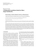
Figure 7: Classification rate as a function of the duration of the
input signal.
filters tuned to extract features at finer orientations, the clas-
sification performance improves significantly. For example,
with seven directional filters, the classification performance
is increased above 98%. However, there is a tradeoff between
the number of filters and classifier performance. As the
number of directional filters increases, the number of free
parameters increases accordingly, thereby increasing the
complexity of the classifier.
4.2. Effect of Time/Frequency Resolution. In the proposed
classification method, the input is a 2D time-frequency
window of the spectrogram; its classification performance is

affected by both the time and frequency resolutions. In order
to determine the optimum input window size, the HICA
should be trained with varying input signal length. One
way of conducting this experiment is to implement several
classification models with different input sizes; however,
this process is computationally expensive as the number of
free parameters of the model is related to the input size.
Another way is to downsample the spectrogram by different
scale f actors along the time-axis and train the classification
method with a fixed input size, for example, 56
× 56. If
the spectrogram is downsampled by a factor k, then for
a56
× 56 input window, the actual length of the input
signal (in seconds) is 2
× 56 × k, where the factor of 2
is due to the sub-sampling operation performed on the
signal before applying the STFT. To reduce aliasing effects
due to downsampling, the spectrogram is smoothed with a
Gaussian filter along the frequency axis and the time axis.
Note that the spectrogram is also downsampled along the
frequency axis so that the periodic peaks are captured by
the input window. Figure 7 records the performance of the
proposed method with respect to the duration of the input
signal. The plot indicates that the maximum classification
rate is obtained with a window length of 4.7 seconds. It is
worth noting that the spectrogram of 4.7 seconds window
contains the walking motion together with the periodicity of
the arm swings, as shown in Figure 6. For a shorter window,
for example, 2.3 seconds, the classification rate is 88%. In

principle, the classification performance should improve as
the window length increases (more information is available
to the classifier). However, the plot shows a decrease in
classification performance; this is because to process a longer
signal, the spectrogram has to be severely downsampled,
leading to loss of vital information from the input window.
Another experiment was also conducted to investigate
the influence of the STFT frequency resolution on the
classification performance. Different window lengths are
used to compute the spectrogram, starting from 64 msec
to 960 msec. We should note that although the frequency
resolution improves with the length of the STFT window, the
spectrogram becomes blurry in time (see Figure 8). In order
to determine the “optimum” frequency resolution, we train
and test several HICAs using different STFT window lengths.
Figure 9 shows the tradeoff between time and frequency
resolution of STFT on the classification performance. With
either good time resolution or good frequency resolution,
the proposed method achieves moderate classification rates.
At 512 msec, the classification method achieves the best
classification accuracy. This implies that to classify human
motions from spectrogram, a balance of good time and
frequency resolution is required.
8 EURASIP Journal on Advances in Signal Processing
Time (seconds)
Doppler frequency (Hz)
246810
−200
−150
−100

−50
0
50
100
150
200
(a)
Time (seconds)
Doppler frequency (Hz)
246810
−200
−150
−100
−50
0
50
100
150
200
(b)
Time (seconds)
Doppler frequency (Hz)
246810
−200
−150
−100
−50
0
50
100

150
200
(c)
Time (seconds)
Doppler frequency (Hz)
246810
−200
−150
−100
−50
0
50
100
150
200
(d)
Figure 8: Spectrograms obtained using different Hamming window lengths: (a) 64 msec, (b) 256 msec, (c) 512 msec, and (d) 960 msec.
64 128 192 256 320 384 448 512 576 640 704 768 832 896 960
70
75
80
85
90
95
100
STFT window length (msec)
Classification rate (%)
Figure 9: Classification rate with respect to the time resolution of
the spectrogram.
4.3. Performance of the Feature Extraction Stages. The pro-

posed method comprises two feature extraction stages: Stage
1 extracts elementary features using nonlinear directional
filters whereas Stage 2 employs adaptive nonlinear filters to
refine the feature extraction process. The outputs of seven
directional filters applied to the Doppler spectrogram of one-
arm motion are presented in Figure 10. The figure shows how
the different filters emphasize the details of the spectrogram
in different directions. This is clearly highlighted by the
output responses of the directional filters. For example, at
0
◦
orientation, the filter differentiates along the horizontal
direction, thereby emphasizing the vertical features. The
outputs of the adaptive filters of Stage 2 are presented in
Figure 11. It is clear from the figure how the micro-Doppler
features of the spectrogram are fur ther underlined in Stage 2.
To determine the effectiveness of the extracted features
for classification, a linear classifier is trained separately on
the inputs computed from the raw spectrogram (input
windows), Stage 1 features, and Stage 2 features. The results
presented in Table 1 show that it is more reliable to classify
features extrac ted by the HICA than the raw spectrogr am
input. Based on the “raw” spectrogram input, a linear
EURASIP Journal on Advances in Signal Processing 9
(a) Original (b) Output map at 0 radian (c) Output map at π/7 radian (d) Output map at 2π/7 radian
(e) Output map at 3π/7 radian (f) Output map at 4π/7 radian (g) Output map at 5π/7 radian (h) Output map at 6π/7 radian
Figure 10: Outputs of Stage 1 filters for one-arm spectrogram input.
Table 1: Classification accuracy of a linear classifier using as input
the features extracted at different stages.
Classification rate

Training set Test set
Features extracted from spectrogram 100% 49.6%
Features extracted from Stage 1 100% 71.0%
Features extracted from Stage 2 100% 98.8%
Table 2: Confusion matrix for classification rates of the three
human motions collected at 0
◦
incidence angle.
NAM P AM FAM
No arms (NAM) 99.4% 0.6% 0%
One arm (PAM) 0.2% 99.8% 0%
Two arms (FAM) 0% 2.7% 97.3%
classifier can merely achieve 49.6% on the test set. However,
using the features extracted by the nonlinear filters in the first
stage, the classification rate is improved to 71.0%. Further
processing by the adaptive filters in Stage 2 yields 98.8%
classification accuracy.
For further analysis, a confusion matrix of the HICA is
depicted in Table 2. The main diagonal of the matrix lists
the correct classification rate for each human motion. The
off-diagonal entries indicate misclassification rates. Entries
in the third row show that the proposed method has some
difficulty in distinguishing between partial arm motion
(PAM) and free-arm motion (FAM). However, the overall
result indicates that the HICA is an effective classification
method for human motions from Doppler spectrograms.
4.4. Comparison with Other Classifiers. In this subsection,
the performance of the proposed HICA method is compared
Table 3: Classification performances of different classifiers using
the spectrogram as input.

Approach Classification rate
Proposed method 98.8%
MLP with one hidden layer 79.7%
SVM 88.0%
with those of two well-known classifiers, namely multilayer
perceptron (MLP) and Support Vec tor Machi ne (SVM).
Herein, we employ the SVM toolbox de veloped by Chang
and Lin [30]. The parameters of the SVM w ith RBF kernel
are obtained by performing a grid-search on C and γ using
cross-validation based on the training set whereas for MLP
severalnetworkswithdifferent number of sigmoid neurons
in the hidden layer are trained, and the network with the best
classification performance on the validation set is selected.
For MLP and SVM, the training and testing samples are pre-
processed by the contrast normalization technique given by
(9). Table 3 lists the best classification results of the MLP and
SVM, together with those obtained by the proposed method.
The SVM and MLP achieve 88% and 79.7% classification
rates, respectively, whereas the proposed method has 98.8%
classification rate. It is clear from these results that the
HICA has better performance than the MLP and SVM. In
[10], for example, the authors computed six salient features
from the spectrogram and used them as input to the SVM.
However, this approach relies on the expert knowledge of the
user to extract the best features possible. In the proposed
approach, the feature extraction process is automatically
handled during training.
4.5. Classification of Short-Time Segments. Several existing
methods use the entire frame to classify the motion of
10 EURASIP Journal on Advances in Signal Processing

(a) Original (b) F1 (c) F2
(d) F3 (e) F4 (f) F5
(g) F6 (h) F7 (i) F8
(j) F9 (k) F10 (l) F11
(m) F12 (n) F13 (o) F14
Figure 11: Outputs of Stage 2 filters for one-arm spectrogram
input.
a subject. For example, Mobasseri and Amin [11] used
principal component analysis (PCA) on the same data set
to extract features from the spectrogram and applied a
quadratic classifier based on the mahalanobis distance for
classifying the spectrogram of human motion. When extract-
ing feature vector parallel to the frequency axis, they achieved
82.5% for classifying no-arm motion (NAM), 69.1% for
classifying PAM and, 70.7% for classifying FAM. However,
when the feature vectors are computed parallel to the time
axis (Doppler snapshots), the classification performance is
increased to 100% for PAM, 98.3% for FAM, and 100%
for NAM. This improvement is due to large changes in the
Doppler frequency across time.
The proposed classification method, on the other hand,
has the capability to classify short-time windows, segments
or the entire frame (spectrogram). Herein, a segment of
the spectrogram is defined as a set of overlapping short-
time windows and the entire frame is represented as a set
of overlapping segments. Based on the optimum window
4.74.95.15.35.55.75.96.16.36.56.76.9
98.6
98.8
99.2

99.4
99.6
99.8
99
100
Time duration of the input segment (sec)
Classification rate (%)
Figure 12: Classification rate as a function of the time duration of
the input segment.
size (4.7 sec), a segment of the spectrogram is classified
by processing its overlapping windows to produce a set
of classification scores, which are then aggregated using
the majority voting rule. Figure 12 shows the accuracy
of the proposed method of classifying input segment of
different lengths. For example, an input segment of 4.7 sec
(i.e., the same time duration as a short-time window), the
classification rate is 98.8%, and increasing the length of
the segment to 5.54 sec, the classification rate increases to
99.37%. Perfect classification is achieved when the length of
the segment is 6.22 sec. Applying the majority voting rule on
the classification scores of all short-time windows extracted
from the entire frame, the proposed method achieves perfect
result in classifying the Doppler spectrogram.
4.6. Oblique View Angle: 30
◦
to the Axis of the Antenna. In
practical situations, the target can move at any directions
with respect to the radar system. As the aspect angle increases
from 0
◦

to 90
◦
, the Doppler signal that returns from the
arm further from the radar becomes weaker due to the
body occlusion; this problem is depicted in Figures 4(b) and
13. With the micro-Doppler signature of one arm subdued,
classification errors are likely to rise. In this experiment, we
assume that Stages 1 and 2 have already been designed to
extract salient features; in this case, the adaptive filters of
Stage 2 are trained on the 0
◦
motion with a linear classifier.
Here, only the classifier is retrained and tested on radar data
collected at 30
◦
to the axis of the radar. The training samples
are from Subjects A and B, and the test samples are from
Subjects C, D, and E. Three classifiers were considered: a
linear, MLP, and SVM classifier. For short-time windows, the
classification performances of the three classifiers are given in
Table 4. Based on a linear classifier, only 77.4% classification
rate is achieved when classifying arm motions collected at an
oblique angle. Using a nonlinear classifier, such as the MLP
or SVM, the classification performance is improved to over
80%. From the confusion matrix, depicted in Table 5, the
HICA method with a MLP classifier achieves 91.2% for FAM,
whereas for PAM and NAM, the classification rates are 77.3%
and 88.2%, respectively. However, when the spectrogram is
EURASIP Journal on Advances in Signal Processing 11
Time (seconds)

Doppler frequency (Hz)
1
2345678910
−200
−150
−100
−50
0
50
100
150
200
(a)
Time (seconds)
Doppler frequency (Hz)
1
2345678910
−200
−150
−100
−50
0
50
100
150
200
(b)
Figure 13: Spectrogr ams of two-arms and no-arms motions
captured at 30 degree incidence angle.
Table 4: Classification rates for 30

◦
data, using features trained with
0
◦
data.
Classifier Average classification rate
Linear classifier 77.4%
MLP classifier 85.5%
SVM classifier 80.9%
Table 5: Confusion matrix for classification rates of three human
motions at 30
◦
using a MLP as classifier in Stage 3 of HICA.
NAM P AM FAM
No arms (NAM) 88.2% 11% 0.78%
One arm (PAM) 12.7% 77.3% 10%
Two arms (FAM) 2.35% 6.47% 91.2%
divided into a set of 170 overlapping short-time windows and
a majority voting rule is applied on their classification scores,
the entire frame is correctly classified.
5. Conclusion
A three-stage classification method employing both fixed
directional and adaptive filters, in addition to a linear
classifier, is introduced for classifying various types of
human walking. The filters are applied in the time-frequency
domain w h ich depicts the Doppler signal power distribution
over time and frequency. Three types of ar m motion are
considered: free-arm swings, one-arm confined swings, and
two-arm confined swings. The proposed method determines
the optimum time-frequency window for training and

testing, and is able to detect and extract distinct Doppler
features from the spectrogram. The data used for testing
and training correspond to five subjects moving towards
and away from the radar with 0
◦
and 30
◦
aspect angle,
and with nonobstructed line of sight. The paper shows
the importance of each stage of the classification method
in improving the classification rates. The attractiveness of
the proposed method lies in its robustness to data mis-
alignments, for ward/backward walking motions, including
the acceleration-deceleration phases exhibited when turning,
and to the specific quadratic distribution used for time-
frequency signal representations.
Acknowledgment
This work is supported in part by a grant from the Australian
Research Council (ARC).
References
[1] J. L. Geisheimer, E. F. Greneker, and W. S. Marshall, “High-
resolution Doppler model of the human gait,” in Radar Sensor
Technology and Data Visualization, vol. 4744 of Proceedings of
SPIE, pp. 8–18, Orlando, Fla, USA, April 2002.
[2] P. Van Dorp and F. C. A. Groen, “Human walking estimation
with radar,” IEE Proceedings: Radar, Sonar and Navigation, vol.
150, no. 5, pp. 356–366, 2003.
[3] V. C. Chen, “Analysis of radar micro-Doppler signature with
time-frequency transform,” in Proceedings of IEEE Signal
Processing Workshop on Statistical Sig nal and Array Processing

(SSAP ’00), pp. 463–466, Pocono, Pa, USA, 2000.
[4]G.E.Smith,K.Woodbridge,andC.J.Baker,“Multistatic
micro-Doppler signature of personnel,” in Proceedings of IEEE
Radar Conference (RADAR ’08), May 2008.
[5] L. Cohen, Time-Frequency Analysis, Prentice Hall, Upper
Saddle River, NJ, USA, 1995.
[6] M. Amin and K. Sarabandi, “Special issue on remote sensing of
building interior,” IEEE Transactions on Geoscience and Remote
Sensing, vol. 47, no. 5, pp. 1267–1268, 2009.
[7] M. Amin, “Special issue on advances in indoor radar imaging,”
Journal of the Franklin Institute, vol. 345, no. 6, pp. 556–722,
2008.
[8] S. E. Borek, “An overview of through the wall surveillance for
homeland security,” in Proceedings of the 34th Applied Imagery
and Pattern Recognition Workshop: Multi-Modal Imaging,pp.
42–47, October 2005.
[9] A. Hunt, “Image formation through walls using a distributed
radar sensor array,” in Proceedings of the 32nd Applied Imagery
Pattern Recognition Workshop, pp. 232–237, 2003.
12 EURASIP Journal on Advances in Signal Processing
[10] Y. Kim and H. Ling, “Human activity classification based on
micro-Doppler signatures using a support vector machine,”
IEEE Transactions on Geoscience and Remote Sensing, vol. 47,
no. 5, Article ID 4801689, pp. 1328–1337, 2009.
[11] B. G. Mobasseri and M. G. Amin, “A time-frequency classifier
for human gait recognition,” in Optics and Photonics in Global
Homeland Security V and Biometric Technology for Human
Identification VI, vol. 7306 of Proceedings of SPIE, Orlando, Fla,
USA, April 2009.
[12] B. Lyonnet, C. Ioana, and M. Amin, “Human gait classification

using micro-Doppler time-frequency signal representations,”
in Proceedings of IEEE International Radar Conference (RADAR
’10), Washington, DC, USA, May 2010.
[13] F. H. C. Tivive, A. Bouzerdoum, S. L. Phung, and K. M.
Iftekharuddin, “Adaptive hierarchical architecture for visual
recognition,” Applied optics, vol. 49, no. 10, pp. B1–B8, 2010.
[14] S. J. Mitchell and R. A. Silver, “Shunting inhibition modulates
neuronal gain during synaptic excitation,” Neuron, vol. 38, no.
3, pp. 433–445, 2003.
[15] S. A. Prescott and Y. D e Koninck, “Gain control of firing rate
by shunting inhibition: roles of synaptic noise and dendritic
saturation,” Proceedings of the National Academy of Sciences of
the United States of America, vol. 100, no. 4, pp. 2076–2081,
2003.
[16] G. Arulampalam and A. Bouzerdoum, “A generalized feed-
forward neural network architecture for classification and
regression,” Neural Networks, vol. 16, no. 5-6, pp. 561–568,
2003.
[17] G. Arulampalam and A. Bouzerdoumn, “Training shunting
inhibitory artificial neural networks as classifiers,” Neural
Network World, vol. 10, no. 3, pp. 333–350, 2000.
[18] A. Bouzerdoum, “Classification and function approximation
using feed-forward shunting inhibitory artificial neural net-
works ,” in Proceedings of the International Joint Conference on
Neural Networks (IJCNN ’00), pp. 613–618, July 2000.
[19] H. N. Cheung, A. Bouzerdoum, and W. Newland, “Properties
of shunting inhibitory cellular neural networks for colour
image enhancements,” in Proceedings of the 6th International
Conference on Neural Information Processing, vol. 3, pp. 1219–
1223, 1999.

[20] T. Hammadou and A. Bouzerdoum, “Novel image enhance-
ment technique using shunting inhibitory cellular neural
networks,” IEEE Transactions on Consumer Electronics, vol. 47,
no. 4, pp. 934–940, 2001.
[21] R. H. Bamberger and M. J. T. Smith, “A filter bank for the
directional decomposition of images: theory and design,” IEEE
Transactions on Signal Processing, vol. 40, no. 4, pp. 882–893,
1992.
[22] S I. Park, M. J. T. Smith, and R. M. Mersereau, “Improved
structures of maximally decimated directional filter banks for
spatial image analysis,” IEEE Transactions on Image Processing,
vol. 13, no. 11, pp. 1424–1431, 2004.
[23] T. T. Nguyen and S. Oraintara, “A class of multiresolution
directional filter banks,” IEEE Transactions on Signal Process-
ing, vol. 55, no. 3, pp. 949–961, 2007.
[24] T. C. Folsom and R. B. Pinter, “Primitive features by steering,
quadrature, and scale,” IEEE Transactions on Pattern Analysis
and Machine Intelligence, vol. 20, no. 11, pp. 1161–1173, 1998.
[25] A. C. Bovik, M. Clark, and W. S. Geisler, “Multichannel texture
analysis using localized spatial filters,” IEEE Transactions on
Pattern Analysis and Machine Intelligence, vol. 12, no. 1, pp.
55–73, 1990.
[26] M. H. Hagan and M. B. Menhaj, “Training feedforward
networks with the Marquardt algorithm,” IEEE Transactions
on Neural Networks, vol. 5, no. 6, pp. 989–993, 1994.
[27] F. H. C. Tivive and A. Bouzerdoum, “Efficient training
algorithms for a class of shunting inhibitory convolutional
neural networks,” IEEE Transactions on Neural Networks, vol.
16, no. 3, pp. 541–556, 2005.
[28] F. H. C. Tivive and A. Bouzerdoum, “A gender recognition

system using shunting inhibitory convolutional neural net-
works ,” in Proceedings of the International Joint Conference on
Neural Networks (IJCNN ’06), pp. 5336–5341, July 2006.
[29] F. H. C. Tivive and A. Bouzerdoum, “A hierarchical learning
network for face detection with in-plane rotation,” Neurocom-
puting, vol. 71, no. 16–18, pp. 3253–3263, 2008.
[30] C C. Chang and C J. Lin, “LIBSVM: a library for
support vector machines,” 2001, />∼cjlin/libsvm/.