Báo cáo sinh học: " Research Article Improved Noise Minimum Statistics Estimation Algorithm for Using in a Speech-Passing Noise-Rejecting Headset" pptx

Hindawi Publishing Corporation
EURASIP Journal on Advances in Signal Processing
Volume 2010, Article ID 395048, 11 pages
doi:10.1155/2010/395048

Research Article
Improved Noise Minimum Statistics Estimation Algorithm for
Using in a Speech-Passing Noise-Rejecting Headset
Saeed Seyedtabaee and Hamze Moazami Goodarzi
Department of Electrical Engineering, Engineering Faculty, Shahed University, P.O. Box 18155/159, Tehran, Iran
Correspondence should be addressed to Saeed Seyedtabaee,
Received 23 August 2009; Revised 7 March 2010; Accepted 8 May 2010
Academic Editor: Igor Djurovi´
c
Copyright © 2010 S. Seyedtabaee and H. Moazami Goodarzi. This is an open access article distributed under the Creative
Commons Attribution License, which permits unrestricted use, distribution, and reproduction in any medium, provided the
original work is properly cited.
This paper deals with configuration of an algorithm to be used in a speech-passing angle grinder noise-canceling headset. Angle
grinder noise is annoying and interrupts ordinary oral communication. Meaning that, low SNR noisy condition is ahead. Since
variation in angle grinder working condition changes noise statistics, the noise will be nonstationary with possible jumps in its
power. Studies are conducted for picking an appropriate algorithm. A modified version of the well-known spectral subtraction
shows superior performance against alternate methods. Noise estimation is calculated through a multi-band fast adapting scheme.
The algorithm is adapted very quickly to the non-stationary noise environment while inflecting minimum musical noise and
speech distortion on the processed signal. Objective and subjective measures illustrating the performance of the proposed method
are introduced.

1. Introduction
Industrial site noises jeopardize workers health condition.
To alleviate the risk, a passive protecting headset may be
worn. It gives good attenuation of ambient noise in the upper
frequency band and some how medium protection in below

500 Hz. Along with the noise, the oral communication link is
also disrupted that should not be.
To improve the working condition, a type of active
headset is designed that allows receiving speech while its
capacity in reducing noise is still in place. The headset in its
simplest form consists of a microphone, a battery-powered
processing unit, and one speaker in one of the ear cups (or
separate sets of microphone, processing unit, and speaker,
one for each ear cup) as shown in Figure 1.
Microphone may receive noise, speech, or noisy speech
signal. The processing unit is expected to enhance the speech
signal and to reduce the noise in any case.
Speech enhancement is one of the most important topics
in signal processing. Enhancement techniques can be classified into single and multichannel classes. Single-channel
systems are the most common real-time scenario algorithms,

since the second channel is not available in most of the
applications, for example mobile communication, hearing
aids, speech recognition systems, and the case of speechpassing noise-canceling headset. The single-channel systems
are easy to build and comparatively less expensive than the
multiple input systems. Nevertheless, they constitute one of
the most difficult situations of speech enhancement, since
no reference signal is available, and clean speech cannot be
statistically preprocessed prior to getting affected by noise.
Wide variety of algorithms has been developed for single
microphone speech enhancement. In waveform filtering class,
only limited assumptions are made about the specific nature
of the underlying signal. The most prominent examples of
waveform processing are the spectral subtraction method
[1], spectral or cepstral restoration [2], Wiener filter [3], the

Wiener filtering extensions [4, 5], and adaptive filtering type
[6].
Other examples include schemes that employ wavelets
[7], modifications of the iterative Wiener filter and the
Kalman filter [8, 9]. Perceptual Kalman filtering for speech
enhancement in [10, 11] and Rao-Blackwellized particle
filtering (RBPF) in [12] are elaborated.


2
Nondiagonal time-frequency estimators that introduce
less musical noise backing up with an adaptive audio block
threshold setting algorithm have been studied in [13].
In stochastic model-based denoising methods, a stochastic parametric model for a speech signal is used instead of
a general waveform model. One statistical model method
is discussed in [14]. Accurate modeling and estimation of
speech and noise via Hidden Markov Models are proposed in
[15]. A minimum mean square error approach for denoising
that relies on a combined stochastic and deterministic speech
model is discussed in [16]. Formant tracking linear prediction (LP) model for noisy speech processing is reported in
[17].
Among all this wide range of methods, the spectral
subtraction-based algorithm is known for its (1) simplicity
in implementation, (2) high power in eliminating noise, and
(3) high speed. The most important problems with spectral
subtraction are speech distortion and residual noise that is
called musical noise. These problems are due to nonaccurate
noise estimation in each frame and differences between the
estimated clean and original signal.
A very challenging task of spectral subtraction speech

enhancement algorithms is noise spectrum estimation. Originally, it requires the silent period to be detected. An algorithm that does not require explicit speech/pause detection
and can update noise estimate even from noisy speech sections is proposed in [18]. The algorithm is based on finding
the minimum statistics of noisy speech for each subband over
a time window. Its major drawback is that when the noise
floor jumps, it takes slightly more one window length to
update the noise spectrum estimate. Updating continuously
the noise estimate is suggested in [19]. However, the
algorithm cannot distinguish between a rise in noise power
and a rise in speech power. In the algorithm, there is a very
sophisticated formula for computing gain factors for each
subband. The gain factors overestimate the noise and permit
gradual suppression of certain subbands as their speech
contribution decreases. Hirsch and Ehrlicher [20] produce
subband energy histograms from past spectral values below
the adaptation threshold over a duration window and choose
the maximum noise level to update the noise estimate. The
major drawback of their method is that it fails to update
the noise estimate when the noise floor increases abruptly
and stays at that level. The method proposed in [21] uses
a recursive equation to smooth and update noise power
estimate with a smoothing parameter related to a priori
SNR. This method needs more time to estimate the noise,
especially when the noise floor jumps. The drawback of
the algorithm in [22] is its large latency. Some improved
algorithms have been proposed in [23–25]. These also suffer
from the similar problem. The authors in [26] propose an
algorithm based on temporal quantile and make use of the
fact that even within speech sections of input signal, not
all frequency bands are permanently occupied with speech.
Rather, for a significant percentage of time the energy within

each frequency band equals the noise level. This method
suffers from computational complexity and requires higher
memory and therefore is not really recommended for realtime systems.

EURASIP Journal on Advances in Signal Processing

Speaker
Ear cup

Processing unit

Sound
absorbing
material
Microphone

Figure 1: The proposed headset.

A method that most fits our speech-passing noiserejecting headset design is the one that (1) renders acceptable
results, (2) has low computational cost, and (3) enjoys
simplicity in implementation. Our primary goal is the design
of a headset that combats the angle grinder noise. Of course,
it can be easily extended to the other rotating devices noise.
From this point of view, the adaptive notch filter method
was thoroughly investigated. Even though, the case is similar
to the problem discussed in [6]; in this case, the application
of various types of adaptive notch filter remained fruitless.
The improvement of spectral subtraction was the
next attempt [27]. Improved spectral subtraction method
appeared strong in forming effective algorithm for rejection

noise. The algorithm embodies fast adapting capability, as
sharp change in angle grinder noise characteristics is noticed.
Using subwindows makes noise estimate updating faster
and enables tracking jumps in the noise power. Another
point is that a priori qualitative coarse knowledge of the
spectrum of the angle grinder noise is easily available that
can be incorporated into the algorithm. This led us to
the proposed combined multiband fast adapting spectral
subtraction method. Angle grinder noise spectrum is not
flat, so multiband noise minimum statistics estimation is
implemented. This is inevitably required for the developing
of an algorithm that takes the musical noise and speech
distortion under control.
This paper reports our latest achievements. In Section 2,
we analyze angle grinder noise. The adaptive notch is
discussed in Section 3. The spectral subtraction is reviewed
in Section 4. In Section 5, our noise estimation algorithm
is disclosed. Performance evaluation is presented in Section 6. Section 7 contains the experimental set-up and the
test results. Finally, conclusion in Section 8 ends up this
discussion.

2. Angle Grinder Noise Analysis
Angle grinder acoustic noise specs change as the device
engagement condition with a part varies. The characteristics
of the noise also depend on the brand and size of angle
grinder. The material of the engaged part also contributes to
the generated sound, as each part generates sound of its own.
Figure 2 shows the noise waveform of a typical angle grinder.

EURASIP Journal on Advances in Signal Processing

3

3. Adaptive Notch Filter Method

1

Amplitude

0.5

0

−0.5

−1

0

4

8
Time (s)

12

16

Figure 2: Waveform of a typical angle grinder noise.

Frequency (KHz)

4

From the analysis of angle grinder noise, it is discovered
that some of the energy is concentrated in specific frequency
components and their harmonics. In line with this type
of analysis, we use adaptive notch algorithm discussed in
[6]. The algorithm is adaptive and is able to track change
in frequency variations. The system employs a cascade of
three second-order adaptive notch/band-pass filters based
on Gray-Markel lattice structure. This structure ensures
the high stability of the adaptive system. A Newton type
algorithm is used for updating the filter coefficients that
enjoy fast adaptation. In addition, a new algorithm using
adaptive filtering with averaging (AFA) is also verified. The
main advantages of AFA algorithm could be summarized
as follows: high convergence rate comparable to that of the
recursive least squares (RLSs) algorithm and at the same time
low computational-complexity.
Adaptive noise-canceling systems are often two channel
types, in which one channel is dedicated to the noisy signal
and the other captures the reference signal. In modification
to the adaptive systems, when a priori knowledge of the
noise fundamental frequency exists, coarse value of the
fundamental frequency is introduced to the algorithm; this
obviates further need to the reference signal, and a single
microphone adaptive system gets applicable.

4. Spectral Subtraction Method
2

0

The main assumption in the spectral subtraction method
is that the speech signal is corrupted by an uncorrelated
additive noise. This is a true assumption in the most realworld cases. A speech signal s(n) that has been degraded
by an uncorrelated additive noise signal n(n) is written as
follows:
0

4

8
Time (s)

12

16

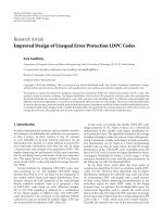
Figure 3: Angle grinder noise spectrograph.

Spectral content of the angle grinder noise is an important factor to be considered in the development of our noise
removal system. The noise spectrum is typically comprised of
a wide-band section and some peaks that have been referred
to as a periodic part plus its harmonics. Figure 3 shows the
spectrograph of the angle grinder noise. Dark lines indicate
existence of strong frequency components in the spectrum.
The frequency is related to the rotation speed of the angle

grinder.
It also reveals that the noise is wide band and each
frequency bin contains some of the noise power. The noise
spectrum is not flat. Variation in noise spectrum due to
change in working condition is apparent from Figure 3.
Major frequency components of the noise change in both
amplitude and frequency. Generation of new frequency
components is apparent from the spectrograph. Change
in noise spectrum means that we are facing a type of
nonstationary behavior.

x(n) = s(n) + n(n).

(1)

The other assumption is that the noise power spectrum in
each window W is a slowly varying process; thus it can be
assumed stationary in each window. The power spectrum of
the noisy signal in window W can be represented by
2

2

|Xw (k)| = |Sw (k)| + |Nw (k)|

2

∗
+ Sw (k)Nw (k) + S∗ (k)Nw (k),
w

(2)

∗
where S∗ (k) and Nw (k) represent the complex conjugate of
w
Sw (k) and Nw (k), respectively. The functions |Sw (k)|2 and
2
|Nw (k)| are referred to as the short-time power spectrum
of the speech and noise, respectively. Here, the short-term
Fourier transform (STFT) of Xw (k) is obtained by

N −1

Xw (k) =

x(λR + n)W(n)e− j2π(kn/N)
(3)

n=0

= |Xw (λ, k)|e

jΦ(λ,k)

,

where λ, N, and 100 × (N − R)/N are the frame index, the
frame length, and the overlapping percentage, respectively.
Φ(λ, k) is the phase of the corrupted noisy signal.

4

EURASIP Journal on Advances in Signal Processing

∗
In (2), the term |Nw (k)|2 , cross-terms Sw (k)Nw (k) and
Sw (k)Nw (k) cannot be obtained directly and are approxi∗
mated by E[|Nw (k)|2 ], E[Sw (k)Nw (k)], and E[S∗ (k)Nw (k)].
w
Where E[·] denotes the expectation operator. If we assume
that n(k) is zero mean and uncorrelated with s(k), then the
∗
cross-terms E[Sw (k)Nw (k)] and E[S∗ (k)Nw (k)] are reduced
w
to zero. Thus, from the above assumptions, the estimate of
the clean speech is given by
∗

2

Sw (k)

2

2

= |Xw (k)| − E|Nw (k)| .

(4)

Typically, E[|N(k)|2 ] is estimated during the silent periods
2
and denoted by |N(k)| . With respect to the assumption that
2
the noise is stationary in each window, |N(k)| is regarded as
the noise power estimate.
To construct the denoised signal, two steps are undertaken. First, the estimated noise minimum statistics amplitude is reduced from the noisy speech spectrum amplitude.
In the second step then, the result is combined with the
phase of the noisy speech signal spectrum. The described
operations are managed through using an inverse discrete
Fourier transform that yields the processed denoised signal
as follows
sw (n) = IDFT

Sw (k) e

jΦ(k)

.

(5)

The phase of the noisy signal is not modified since human
perception is not sensitive to the phase [28]. However, in
a recent work [29], the authors have shown that at lower
SNRs, below 0 db, the phase error causes considerable speech
distortion.
Since the average magnitude of an instantaneous noise

spectrum does not follow truly sharp peaks of the noise, an
annoying residual noise, called musical noise, appears after
applying spectral subtraction method. Most of the research
in the past decade has been focused on the ways to combat
the problem of the musical noise. It is literally impossible to
minimize musical noise without affecting the speech quality,
and hence, there should be a trade-off between the amount
of noise reduction and speech distortion.
The proposed method in [30] is one of the earliest
methods to reduce residual noise. Modifications that we
made to the original spectral subtraction method are (1)
subtracting an overestimate of the noise power spectrum
and (2) preventing the resultant spectrum from going below
a preset minimum level (spectral floor). The proposed
algorithm is expressed by
Sw (k)
=

the segmental noisy signal to noise ratio (NSNR) that is
calculated for every frame by:
⎡
⎢

SNRi = 10 log⎣

ei
k=bi
ei
k=bi

⎤
2
|Xi (k)| ⎥
2 ⎦,

(7)

Ni (k)

where bi and ei are the beginning and ending frequency bins
of the ith frequency band. In this definition, it is allowed that
the overall frequency band divided into several subbands.
The oversubtraction factor α is calculated by
⎧
⎪1
⎪
⎪
⎪
⎪
⎨

NSNR ≥ 20 dB,

α = ⎪α0 − 3 NSNR −5dB ≤ NSNR ≤ 20 dB,
⎪
20
⎪
⎪
⎪
⎩5

NSNR ≤ −5 dB,

(8)

where α0 = 4 is the desired value of α at 0 db NSNR.

5. Noise Minimum Statistics Estimation:
The Proposed Multiband Fast Adaptive
Algorithm
5.1. The Initial Algorithm:The Martin’s Method. A very
challenging task of spectral subtraction speech enhancement
algorithms is noise spectrum estimation. For estimating
stationary noise specifications, the first 100–200 ms of each
noisy signal are usually assumed pure noise and used to
estimate the noise for over the time [31]. For estimation of
nonstationary noise, the noise spectrum needs to be estimated and updated continuously. To do so, we need a voice
activity detector (VAD) to find silence frames for updating
noise estimation [32]. In a nonstationary noise case or low
SNR situations, nonspeech/pause section detection reliability
is a concern. In [18], the author proposes an algorithm that
does not require explicit speech/pause detection and can
update noise estimation even from noisy speech sections.
The minimum statistics noise tracking method is based on
the observation that even during speech activity a short-term
power spectral density estimate of the noisy signal frequently
decays to values that are representative of the noise power
level. Thus, by tracking the minimum power within finite
(D) PSD frames, large enough to bridge high power speech
segments, the noise floor can be estimated [33].
The smoothed power spectrum of noisy speech Px (λ, k)

is calculated with a first-order recursive equation as follows:
Px (λ, k) = ηPx (λ − 1, k) + 1 − η |X(λ, k)|2 ,

(9)

2

⎧
⎪|Xw (k)|2 − α Nw (k)
⎨
⎪
⎩

β Nw (k)

2

2

2

if |Xw (k)|2 ≥ α Nw (k) ,
else,
(6)

where α is the oversubtraction factor, and β is the spectral
floor parameter. The oversubtraction factor α depends on

where λ and k are the frame and the frequency bin indices,
respectively. η is a smoothing constant where value is to be set

appropriately between zero and one. Often a constant value
of 0.85 to 0.95 is suggested [33].
If x(n) can be assumed stationary with a relatively small
span of correlation and for a large frame size, the real and
imaginary part of the Fourier transform coefficients, X(λ, k),
can be considered independent and modeled as zero mean
Gaussian random variables [34]. Under this assumption,


EURASIP Journal on Advances in Signal Processing

5

7

The corrupted speech

Amplitude

1
6

Mean PSD

5

0
−1

4

0

2

4

6
Time (s)

3

10

12

8

10

12

8

10

12

(a)

2

The initial alg.

1

0

100

200

300
400
500
Frame number

The noisy signal
The original noise

600

700

800

Amplitude

1

0

8

−1

2

4

6
Time (s)
(b)

the true PSD of the noise, can be replaced by
where
its latest estimate, Pn (λ, k). More works on this subject have
recently been reported in [35]. Dependency of the optimal
value of η on λ, k and noise Power Density Frequency (PDF)
increases its computation burden while, its allowable range
(0.85 to 0.95) is limited, and there is uncertainty about
PDF of the (non stationary) noise. This justifies using an
average value that is calculated occasionally, instead of the
nonoptimal exact value computation in each iteration.
5.2. Noise Spectral Minimum Estimation. Since spectrum of
noisy speech signal often decays to the spectrum of noise, we
can get an estimate of the noise in a time window of about
0.8–1.4 s. This corresponds to finding the minimum among
a number (D) of consecutive PSDs, Px (λ, k), as follows:

λD = i ∗ L,

−1

0

2

4

6
Time (s)
(c)

(10)

2
σn (λ, k),

PD min (λD , k) = min Px λD − j, k ,

0

(11)

where i is the estimation iteration number. The calculated
spectral minimum, then, is used in the future frames, (λ >
λD ), for spectral subtraction. The equation may be updated
in every and each λ step, L = 1, then k × (D − 1) compare
operations are needed per step. However, if it is computed

after every D consecutive PSDs, L = D, the number of
compare operations lessens to about k operation per λ step.
In any case, if the current noisy speech power spectrum

Figure 5: Speech signal corrupted with angle grinder noise (a), the
initial method produced signal (b), and our modified de-noising
method output (c).

5

4

3
MOS

1
2,
2
1 + (Px (λ − 1, k))/ σn (λ, k) − 1

The improved alg.

1
Amplitude

each periodogram bin is an exponentially distributed random variable. If the condition holds, an optimal smoothing
constant derived in [33] can be employed that enhances the
performance

j = 0 · · · D − 1,

0

The initial alg.
The improved alg.

Figure 4: The average smoothed PSD of the noisy speech, the noise,
the initial method estimate and our algorithm estimate.

ηopt (λ, k) =

0

2

1

0
1

2

3

4

Listener no.

Figure 6: Comparison of the perceptual quality of the enhanced
speech signals (vertical) by 4 listeners (Horizontal), the dark

column: the initial method, and the light column: the modified
method.


6

EURASIP Journal on Advances in Signal Processing
Table 1: The five-point scale in the Mean Opinion Score.

Rating
5
4
3
2
1

Speech quality
Excellent
Good
Fair
Poor
Unsatisfactory

Levels of distortion
Imperceptible
Just perceptible but not annoying
Perceptible and annoying
Annoying but not objectionable
Objectionable

is smaller than PD min (λD , k), the noise power is updated
immediately:
PD min (λD , k) = min{Px (λ, k), PD min (λD , k)},

λ > λD .
(12)

However, in case of increase in noise power in the current
frame, the update of the noise estimate is delayed by more
than D spectral frames.
The estimate of PD min (λD , k) suffers from bias toward
lower values that has to be compensated
PDn (λD , k) = δmin PD min (λD , k).

(13)

In case of a relatively white x(n), bias compensation equations have been derived in [18, 33], with the one in [33] being
as follows:
δmin (λD , k) ≈ 1 + (D − 1)

var{Px (λ, k)}
,
4
σn (λD − L, k)

PM min , the next D-PSD spectral minimum is derived as
follows:
PDmin (λ D , k) = min{PM min (λD − i × M, k)},
i = 0 · · · C − 1.

(16)

D must be large enough to bridge any peak of speech activity,
but short enough to follow nonstationary noise variations.
Experiments with different speakers and modulated noise
signals have shown that window lengths of approximately
0.8 s–1.4 s give good results [18].
Now, in case of increasing noise power in the current
frame, the update of the noise estimate is delayed by D + M
spectral frames. To speed up the tracking of the noise spectral
minimum, an increase in the importance of the current subframe, with respect to the other past subframes is proposed
PD min (λD , k) = min{δi PM min (λD − i × M, k)},
i = 0 · · · C − 1,

(17)

where δ is a look-ahead constant with δi ≤ δi−1 . At the
simplest case we have δi = 1. Also, for having an accurate
noise spectral minimum estimation when a jump occurs in
noise power, we modify (12) as follows:
PD min (λD , k) = min Px (λ, k), ξPM min (λD + i × M, k) ,

(14)

(18)

where λD − L indicates the time of the previous PDmin estimation. The equation indicates that the compensation constant
is a function of time, λ and frequency bin, k. However, its
exact value will not be optimal for nonstationary situations.
Deriving an average value, occasionally, and using it are a

remedy that circumvents its computational costs and fits its
nonoptimal value.
Incorporating the temporal specs of angle grinder noise
in the algorithm has been elaborated in Section 5.2 while
employing the frequency specs of noise power has been
addressed in Section 5.3.

where ξ is the relation-ahead parameter that is related to the
segmental NSNR and λD + i × M < λ < λD + (i + 1) × M.
At the simplest situation we set ξ = 1. With increasing
the value of δ and ξ, the algorithm can track nonstationary
noises well and the upper bound limit is preventing speech
distortions. The above provisions are in close tie with the
temporal specs of noise spectrum. In case of angle grinder,
change in working conditions from nonengaged (stationary
noise) to start of engagement (jump in noise power) to
engaged (nonstationary) with part and vice versa shapes the
dependency of the spectrum to time.

5.3. Fast Adapting Noise Estimation. To compensate the
noise estimation delay, when the noise power jumps, the
division of a D-PSD block into C-weighted M-PSD block
is considered (D = C × M). It reduces the computational
complexity and makes the adaptation faster [18]. The
decomposition of the D-PSD block into C subblocks has
the advantage that a new minimum estimate is available
after already M samples without a substantial increase in
operations.
The computation steps start with the calculation of the
spectral minimum of the first M frame spectral minimum as

follows:

5.4. Multiband Fast Adapting Noise Spectral Estimation. In
the case of angle grinder noise, the segmental SNR of
high frequency band is significantly lower than the SNR of
low frequency band; it implies that their noise variance is
different. Another important point that should be considered
here is that the high-energy first formant of vowels rests
approximately on the frequency band between 400 and
1000 Hz. As a result, this band is not so much susceptible
to noise spectrum coarse estimation. On the other hand,
the upper frequency band that consonants occupy, the noise
spectral estimate should be as precise as possible; otherwise,
the intelligibility of speech is impaired. For these reasons, to
enhance the performance of our algorithm, we divide the
overall spectrum into four regions (0–400 Hz, 400–600 Hz,
600–1000 Hz, and above), and in compliance with (14),
separate values for δ and ξ are assigned to each of them. This
is somehow similar to the study in [36] regarding colored
noise. By this technique, diverse sensitivities in tracking

PMmin (λD + M, k) = min Px λD + M − j, k ,
j = 0 · · · M − 1.

(15)

Then, PM min for each of the other next M frames is
determined. After the calculation of a set of C number of

EURASIP Journal on Advances in Signal Processing
The clean
Frequency
(KHz)

2
Amplitude

7

0

−2

0

3

6
Time (s)

9

2

4

6
Time (s)

8

10

12

8

10

12

8

10

12

8

10

12

Frequency
(KHz)

The noisy speech

2

0

0

2

4

6
Time (s)
(b)

3

6
Time (s)

9

12
Frequency
(KHz)

0

(b)
The initial alg.

1

The initial alg.

4
2
0

0

2

4

6
Time (s)

0

−1

(c)

0

3

6
Time (s)

9

12

(c)

Frequency
(KHz)

Amplitude

0

4

0

−1

Amplitude

0

(a)

(a)

The improved alg.

4
2
0

The improved alg.

1
Amplitude

2

12

The noisy

1

The clean speech

4

0

2

4

6
Time (s)
(d)

0

−1

Figure 8: Spectra of the clean, corrupted, and enhanced speech.
0

3

6
Time (s)

9

12

(d)
4

Figure 7: Waveform of the clean, corrupted and enhanced speech
signal.

nonstationary noise in the different frequency bands are
employed. Hence, it is expected that reduction in the speech
distortion and increases in the SNR of the processed speech
are achieved. For good performance, lower values for δ and ξ
in the lower bands are suggested.

MOS

3

2

1

6. Performance Evaluation
0

In order to evaluate the performance of any speech enhancement algorithm, it is necessary to have reliable and appropriate means, based on which the quality and intelligibility
of the processed speech can reliably and fairly be quantified.
The measures are divided in two groups, objective and
subjective measures.

1

2

3

4

Listener no.

Figure 9: Comparison of the perceptual quality of the enhanced
speech signals (vertical) by 4 listeners (horizontal), the dark
column: the initial method, and the light column: the modified
method.


8

EURASIP Journal on Advances in Signal Processing
Table 2: Average of SNR and IS values obtained from 24 male and female speech samples.
Angle grinder noise (nonengaged)

SNR
Seg SNR

in
in
the initial
the proposed
in
the initial
the proposed
in
the initial
the proposed

SNR f w

Seg IS

0

5
1.83
5.70
5.82
−7.1
0.75

3.04
1.38
1.31
0.69

−1.3

3.7
4.72
−11.5
−2.29
1.8
2.05
1.78
0.97

10
4.81
7.36
7.36
−2.95
3.26
4.01
0.89
1.02
0.58

6.1. Objective Measures. Segmental SNR is one of the most
famous objective measures that is defined by [21]
⎡

ei
k=bi

⎢

SNRM = 10 log⎣

ei
k=bi

2
|XM (k)|

SM (k) − SM (k)

⎤
⎥

2 ⎦,

(19)

Angle grinder noise (engaged)
0
−1.15

1.76
2.60
−13.2

−6.14
−1.58
3.64
2.74
2.37

5
0.62
3.21
3.6
−10.1
−3.36
0.17
3.15
2.57
2.03

10
3.16
5.07
5.11
−6.01
0.01
2.12
2.50
2.11
1.63

6.2. Subjective Measure. In the subjective measure test, the
quality of an utterance is evaluated by the opinion of

listeners. One of the most often used tests is Mean Opinion
Score (MOS), in which listeners rate the speech quality on a
five-point scale, according to Table 1.

where SM (k) and SM (k) are the clean and estimated speech in
frame M, respectively.
The other method for calculating SNR is based on a
frequency-weighting scheme. This measure better reflects the
human auditory system. It is called the Frequency-weighted
segment-based SNR (SNRfw ) and is defined by

7. Experimental Setup and Results

SNRfw

7.1. Adaptive Notch Filter. The algorithm worked in canceling pure simulated sine signals, but its performance
regarding angle grinder noise was not acceptable. Even
though, there are distinct peaks in the spectrum of the angle
grinder noise, and the algorithm is able to canceling them;
the SNR of the processed signal is not acceptable to be
applicable in the headset design. In fact, 1 db improvement
in SNR does not satisfy what is really needed.
Further analysis of the noise indicates that the quasiperiodic part of the noise does not carry enough percentage of
the noise energy, to the extent that by its removal major
improvement occurs. Therefore, other methods of denoising
must be considered.

=

1

M

M −1

N
k=1 αk

× 10 log[(Es (λ, k))/(Es−s (λ, k))]

λ=0

N
k=1 αk

,

(20)
where Es ( j, n) and Es−s ( j, n) denote the short-term signal
and noise energy in one of the M frames (index by j),
respectively, and the weight αk is applied to each of the N
frequency band indexed by k.
Itakra-Saito (IS) distance is another objective measure
that is usually used and has high degree of correlation
with the subjective measure (r = 0.59) [37]. It performs
a comparison between spectral envelopes (all-pole parameters) and that is more influenced by a mismatch in formant
location than in spectral valleys. The minimum value of IS
corresponds to the best speech quality [27, 29–32, 36, 38].
We use the mean of IS measure that is defined as
d(c1 , c2 ) = 0.5 10 log

c1 R2 c1
cRc
+ 10 log 2 1 2 ,
c2 R2 c2
c1 R1 c1

(21)

where c1 and c2 are the linear prediction coefficient vectors
of the clean and enhanced speech segments, respectively. R1
and R2 are the Toeplitz autocorrelation matrices of the clean
and enhanced speech segment, respectively.
Perceptual Evaluation of Speech Quality (PESQ) enjoys
high degree of correlation with the subjective measures (r =
0.9) but is one of the most computationally complex of all
[39].

Simulations were carried out using 24 Iranian males and
females pieces of speeches. Speech samples are recorded in
the presence of angle grinder noise in (1) engaged, and (2)
non-engaged modes. Signals are sampled at 8 KHz.

7.2. Fast Adaptive Spectral Subtraction. Signal is framed with
an N = 256 samples hamming window with 50% overlap,
R = 128. In the noise estimation section, the time interval for
finding the minimum of noisy speech spectrum is considered
0.72 s, and the number of spectral frames, D, is calculated as
follows:
(D − 1)R + N
= 0.72 s,

fs

(22)

where fs is the sampling frequency. The D = 44 spectral
frames is divided into 4 sections each with 11 spectral frames.
Then, the estimate of the noise using the modified estimator
is computed. We set the values δ1 = 1.01, δ2 = 1.02,
δ3 = 1.03,and ξ = 1.1 based on the experimental results.
Using spectral subtraction with oversubtraction parameter


EURASIP Journal on Advances in Signal Processing

9

Table 3: δ and ξ for each of the frequency bands.

δ1
δ2
δ3
ξ

1 Hz ≤ k <
400 Hz
1
1.01
1.05
1.02

400 ≤ k <
600 Hz
1
1.07
1.08
1.1

600 ≤ k <
1 KHz
1
1.03
1.09
1.03

1 KHz ≤ k
1
1.1
1.12
1.13

α0 = 4 and spectral floor β = 0.002, the clean speech in each
FFT subwindow is obtained and with taking inverse Fourier
transform and overlap and add method, the estimated clean
speech signal in the time domain is derived.
Increase in the spectral floor parameter results in residual
noise contraction and inversely speech signal distortion.
Therefore, an appropriate floor constant (e.g., θ = 0.03) has
to be set for the processed signal. As a result, a considerable
reduction in the musical noise is gained.
Figure 4 shows one bin, k, of the average smoothed PSD

of the noisy speech signal, the original noise, the estimated
noise by the initial method and the one produced by our
improved algorithm. Our method has clearly followed the
original noise spectrum. By setting δ and ξ to one, the results
tend to the one of the initial method.
Figure 5 shows a piece of speech signal corrupted
with a nonstationary angle grinder noise at 0 db SNR, the
processed signal by the initial algorithm and by our improved
algorithm. It is seen that the proposed algorithm can reduce
the noise truly, and the amount of the residual noise is very
low.
Table 2 compares the results obtained from averaging
SNR and IS distance measures from the processed 24 male
and female speech samples. According to Table 2, the value
of mean SNR in the proposed algorithm is increased and the
mean IS distance is considerably decreased, especially when
speech is corrupted with highly nonstationary noise and SNR
is low. The objective results show superiority of our modified
algorithm to the initial algorithm achievements.
To do the subjective test, 3 speech signal samples, each
with length 6 Sec, were corrupted with the engaged angle
grinder noise under various SNRs. The processed speeches
are scored by four listeners. Figure 6 shows the average results
gathered from each listener. The dark column is related to
the initial method, and the light column is related to our
modified method.
As it is shown, the processed speech with the modified
algorithm has better perceptual quality than that of the initial
algorithm.
7.3. Multi Band Fast Adapting Spectral Subtraction. In this

test, the time interval for finding minimum of the noisy
speech spectrum is set to 1.5 s:
(D − 1)R + N
= 1.5 s = D = 92,
⇒
fs

(23)

where N = 256 is the time window length. With 50%
overlapping, R is 128. The D = 92 spectral frame is
subdivided into 4 sections of each with 23 spectral frames.
Then, the estimate of the noise using the modified estimator
is conducted. Based on the experiments, the values of δ and
ξ in (17) and (18) in each four bands are set as indicated in
Table 3.
As you noticed, different values have been set for each of
the 4 frequency bands (low: 1–400 Hz, middle: 400–600 Hz,
600–1000 Hz and above). This accounts for the different
noise power in each section of the angle grinder noise
spectrum. Using spectral subtraction with oversubtraction
parameter α0 = 4 and spectral floor β = 0.002, the
clean speech in each FFT subwindow is obtained. By using
Inverse Fourier Transform and Overlap and Add method, the
estimated clean speech signal in the time domain is derived.
Since with increasing the spectral floor, the residual noise
would decrease at the cost of speech signal distortion, we use
a time floor constant of θ = 0.03. As a result, a considerable
reduction in the musical noise is achieved.
Figures 7 and 8 show the waveform and spectra of a

female speech signal corrupted with a nonstationary angle
grinder noise at 0 db SNR, and the processed signal by the
initial algorithm and the output of the modified multi band
algorithm proposed here. It is viewed that the proposed
algorithm can reduce the noise truly and the amount of
the residual noise is very low. This can be verified better by
listening to the pieces of speeches.
Table 4 shows the results obtained from the average
of SNR, IS distance and PESQ measures for the improved
method in comparison with the initial method. The test
was enhancement of 24 male and female speech samples
corrupted with noises with various SNRs. According to
the Table 4, the values of SNR and the PESQ in the
proposed algorithm have been increased and the IS distance
is considerably decreased, especially for low SNR samples.
The objective results show the advantage of our modified
algorithm performance versus the initial algorithm results.
To do the subjective test, 24 speech signal samples
each with 6-sec-length were corrupted with the engaged
angle grinder noise with various SNRs (0 db to 15 db). The
processed speeches are scored by four listeners. Figure 9
shows the average results gathered from each listener.
The dark column belongs to the initial method, and the
light column is related to our improved method. As it
is shown, the processed speech with the modified algorithm has better perceptual quality than that of the initial
algorithm.
7.4. Overall Assessment. Comparing the contents of Table 2
and Table 4 reveals the outcome gained during this study.
In the 0 db SNR case, the worst case analyzed here, Table 2
indicates that the method has achieved 2.6 db improvement.

The same case in Table 4 shows 6.2 db increase in segmental
SNR. Meaning that multiband algorithm is more fit to
the case than the single frequency band algorithm. The
effectiveness of the algorithm is more noticed in low SNR
situations than in moderate SNR cases.


10

EURASIP Journal on Advances in Signal Processing

Table 4: The mean SNR, PESQ, and IS values obtained from
enhancing 24 noisy male and female speech samples at our
experiments for the proposed method compared to the other
methods for various SNRs.
Input SNR
Seg SNR
In
The initial
The improved
SNR fw
In
The initial
The improved
PESQ mos
In
The initial
The improved
IS
In

The initial
The improved

non engaged
0
5
10
−1 2.4 6.2
3.7 6
8.1
5.5 6.3 6.9
−9 −6 −1
−1 1.3 4.3
3 3.8 4.8
1.4 1.6 1.8
1.5 1.9 2.2
2 2.3 2.4
2.1 1.3 0.7
1.7 1.2 0.9
0.6 0.5 0.4

engaged
0
5
−1.2 1.56
1.7 3.94
6.2 7.22
−13 −8.5
−6.2 −2
2.2

3.8
1.52 1.68
1.29 1.62
1.93 2.19
3.65 2.91
2.77 2.43
1.63 1.42

10
4.49
5.94
8
−4
1.45
5.1
1.92
1.96
2.4
2.22
1.91
1.22

[6]

[7]

[8]

[9]

[10]

[11]

8. Conclusion
In this paper, the spectral subtraction method was used to
reduce nonstationary angle grinder noise from speech signal.
A modified noise estimation algorithm with rapid adaptation
for tracking sudden variations in noise power was proposed,
and its performance was checked using both objective
and subjective measures. It was shown that, the proposed
algorithm using multiband weighted subwindow behaves
faster and renders more accurate estimate of nonstationary
noise and provides a processed signal with minimum musical
noise and speech distortion. More works are underway using
other appropriate methods. Our challenge is obtaining high
quality denoised speech under low SNR situations.

Acknowledgment

[12]

[13]

[14]

[15]

[16]

This work has been partially supported by the Shahed
University research office (SURO), Tehran, Iran.
[17]

References
[1] S. F. Boll, “Suppression of acoustic noise in speech using
spectral subtraction,” IEEE Transactions on Acoustics, Speech,
and Signal Processing, vol. 27, no. 2, pp. 113–120, 1979.
[2] P. Vary and M. Eurasip, “Noise suppression by spectral
magnitude estimation-mechanism and theoretical limits,”
Signal Processing, vol. 8, no. 4, pp. 387–400, 1985.
[3] J. S. Lim and A. V. Oppenheim, “Enhancement and bandwidth
compression of noisy speech,” Proceedings of the IEEE, vol. 67,
no. 12, pp. 1586–1604, 1979.
[4] R. J. McAulay and M. L. Malpass, “Speech enhancement using
a soft-decision noise suppression filter,” IEEE Transactions on
Acoustics, Speech, and Signal Processing, vol. 28, no. 2, pp. 137–
145, 1980.
[5] Y. Ephraim and D. Malah, “Speech enhancement using a
minimum mean-square error short-time spectral amplitude

[18]

[19]

[20]

[21]

estimator,” IEEE Transactions on Acoustics, Speech, and Signal

Processing, vol. 32, no. 6, pp. 1109–1121, 1984.
G. Iliev and K. Egizarian, “Adaptive system for engine noise
cancellation in mobile communications,” Automatica, vol. 34, pp. 137–143, 2004.
Y. Hu and P. C. Loizou, “Speech enhancement based on
wavelet thresholding the multitaper spectrum,” IEEE Transactions on Speech and Audio Processing, vol. 12, no. 1, pp. 59–67,
2004.
A. Mouchtaris, J. Van Der Spiegel, P. Mueller, and P. Tsakalides,
“A spectral conversion approach to single-channel speech
enhancement,” IEEE Transactions on Audio, Speech and Language Processing, vol. 15, no. 4, pp. 1180–1193, 2007.
K. K. Paliwal and A. Basu, “A speech enhancement method
based on Kalman filtering,” in Proceedings of the International
Conference on Acoustics, Speech, and Signal Processing (ICASSP
’87), pp. 177–180.
N. Ma, M. Bouchard, and R. A. Goubran, “Perceptual
Kalman filtering for speech enhancement in colored noise,” in
Proceedings of the IEEE International Conference on Acoustics,
Speech, and Signal Processing (ICASSP ’04), vol. 1, pp. 717–720,
May 2004.
C. H. You, S. Rahardja, and S. N. Koh, “Perceptual Kalman
filtering speech enhancement,” in Proceedings of the IEEE International Conference on Acoustics, Speech and Signal Processing
(ICASSP ’06), vol. 1, pp. 461–464, May 2006.
F. Musti` re, M. Bouchard, and M. Boli´ , “Low-cost modificae
c
tions of Rao-Blackwellized particle filters for improved speech
denoising,” Signal Processing, vol. 88, no. 11, pp. 2678–2692,
2008.
G. Yu, S. Mallat, and E. Bacry, “Audio denoising by timefrequency block thresholding,” IEEE Transactions on Signal
Processing, vol. 56, no. 5, pp. 1830–1839, 2008.
Y. Ephraim, “Statistical-model-based speech enhancement
systems,” Proceedings of the IEEE, vol. 80, no. 10, pp. 1526–

1554, 1992.
D. Y. Zhao and W. B. Kleijn, “HMM-based gain modeling for
enhancement of speech in noise,” IEEE Transactions on Audio,
Speech and Language Processing, vol. 15, no. 3, pp. 882–892,
2007.
R. C. Hendriks, R. Heusdens, and J. Jensen, “An MMSE estimator for speech enhancement under a combined stochasticdeterministic speech model,” IEEE Transactions on Audio,
Speech and Language Processing, vol. 15, no. 2, pp. 406–415,
2007.
Q. Yan, S. Vaseghi, E. Zavarehei et al., “Formant tracking linear
prediction model using HMMs and Kalman filters for noisy
speech processing,” Computer Speech and Language, vol. 21,
no. 3, pp. 543–561, 2007.
R. Martin, “Spectral subtraction based on minimum statistics,” in Proceedings of the 17th European Signal Processing
Conference, pp. 1182–1185, 1994.
G. Doblinger, “Computationally efficient speech enhancement
by spectral minima tracking in subbands,” in Proceedings
of the 4th European Conference on Speech Communication
and Technology (EUROSPEECH ’95), pp. 1513–1516, Madrid,
Spain, September 1995.
H. G. Hirsch and C. Ehrlicher, “Noise estimation techniques
for robust speech recognition,” in Proceedings of the 20th
International Conference on Acoustics, Speech, and Signal
Processing (ICASSP ’04), pp. 153–156, Detroit, Mich, USA,
May 1995.
L. Lin, W. H. Holmes, and E. Ambikairajah, “Subband noise
estimation for speech enhancement using a perceptual Wiener


EURASIP Journal on Advances in Signal Processing

[22]

[23]

[24]

[25]

[26]

[27]

[28]

[29]

[30]

[31]

[32]

[33]

[34]
[35]

[36]

filter,” in Proceedings of the IEEE International Conference on

Accoustics, Speech, and Signal Processing (ICASSP ’03), pp. 80–
83, Hong Kong, April 2003.
I. Cohen and B. Berdugo, “Noise estimation by minima controlled recursive averaging for robust speech enhancement,”
IEEE Signal Processing Letters, vol. 9, no. 1, pp. 12–15, 2002.
S. Rangachari, P. C. Loizou, and Y. Hu, “A noise estimation
algorithm with rapid adaptation for highly non-stationary
environments,” in Proceedings of the IEEE International Conference on Acoustics, Speech, and Signal Processing (ICASSP ’04),
pp. 305–308, May 2004.
N. Fan, J. Rosca, and R. Balan, “Speech noise estimation
using enhanced minima controlled recursive averaging,” in
Proceedings of the IEEE International Conference on Acoustics,
Speech and Signal Processing (ICASSP ’07), vol. 4, pp. 581–584,
April 2007.
D. Farrokhi, R. Togneri, and A. Zaknich, “Single channel
speech enhancement using a 9 Dimensional noise estimation
algorithm and controlled forward march averaging,” in Proceedings of the 9th International Conference on Signal Processing
(ICSP ’08), pp. 17–21, October 2008.
V. Stahl, A. Fischer, and R. Bippus, “Quantile based noise
estimation for spectral subtraction and Wiener filtering,” in
Proceedings of the IEEE Interntional Conference on Acoustics,
Speech, and Signal Processing (ICASSP ’00), vol. 3, pp. 1875–
1878, June 2000.
H. M. Goodarzi and S. Seyedtabaee, “Speech enhancement
using spectral subtraction based on a modified noise minimum statistics estimation,” in Proceedings of the 5th International Joint Conference on INC, IMS and IDC, pp. 1339–1343,
2009.
J. S. Lim and A. V. Oppenheim, “Enhancement and bandwidth
compression of noisy speech,” Proceedings of the IEEE, vol. 67,
no. 12, pp. 1586–1604, 1979.
N. W. D. Evans, J. S. D. Mason, W. M. Liu, and B. Fauve, “An
assessment on the fundamental limitations of spectral subtraction,” in Proceedings of the IEEE International Conference on

Acoustics, Speech and Signal Processing (ICASSP ’06), vol. 1, pp.
145–148, May 2006.
M. Berouti, R. Schwartz, and J. Makhoul, “Enhancement of
speech corrupted by acoustic noise,” in Proceedings of the
IEEE International Conference on Acoustics, Speech, and Signal
Processing (ICASSP ’79), pp. 208–211, April 1979.
C. Cole, M. Karam, and H. Aglan, “Spectral subtraction of
noise in speech processing applications,” in Proceedings of the
40th Southeastern Symposium on System Theory (SSST ’08), pp.
50–53, New Orleans, LA, USA, March 2008.
P. Krishnamoorthy and S. R. Prasanna, “Modified spectral
subtraction method for enhancement of noisy speech,” in
Proceedings of the IEEE 3rd International Conference on
Intelligent Sensing and Information Processing, pp. 146–150,
Bangalore, India, December 2005.
R. Martin, “Noise power spectral density estimation based on
optimal smoothing and minimum statistics,” IEEE Transactions on Speech and Audio Processing, vol. 9, no. 5, pp. 504–512,
2001.
D. R. Brillinger, Time Series: Data Analysis and Theory,
Holden-Day, New York, NY, USA, 1981.
N. Derakhshan, A. Akbari, and A. Ayatollahi, “Noise power
spectrum estimation using constrained variance spectral
smoothing and minima tracking,” Speech Communication, vol.
51, no. 11, pp. 1098–1113, 2009.
S. Kamath and P. Loizou, “A multi-band spectral subtraction
method for enhancing speech corrupted by colored noise,” in

11
Proceedings of the IEEE International Conference on Acoustics,
Speech and Signal Processing (ICASSP ’02), vol. 4, pp. 4160–

4164, Orlando, US, 2002.
[37] S. V. Vaseghi, Advanced Digital Signal Processing and Noise
Reduction, John Wiley & Sons, New York, NY, USA, 2000.
[38] J. R. Deller Jr., J. H. L. Hansen, and J. G. Proakis, Discrete-Time
Processing of Speech Signals, IEEE Press, Piscataway, NJ, USA,
2000.
[39] Y. Hu and P. C. Loizou, “Evaluation of objective quality
measures for speech enhancement,” IEEE Transactions on
Audio, Speech and Language Processing, vol. 16, no. 1, pp. 229–
238, 2008.