Báo cáo sinh học: " Research Article Two-Dimensional Harmonic Retrieval in Correlative Noise Based on Genetic Algorithm" pdf
Bạn đang xem bản rút gọn của tài liệu. Xem và tải ngay bản đầy đủ của tài liệu tại đây (1.12 MB, 10 trang )
Hindawi Publishing Corporation
EURASIP Journal on Advances in Signal Processing
Volume 2010, Article ID 569371, 10 pages
doi:10.1155/2010/569371
Research Article
Two-Dimensional Harmonic Retri eval in Correlative Noise
Based on Genetic Algorithm
Sun-Yong Wu,
1, 2
Gui-Sheng Liao,
1
and Zhi-Wei Yang
1
1
National Lab of Radar Signal Processing, Xidian University, Xi’an, Shanxi 710071, China
2
Department of Computational Science and Mathematics, Guilin University of Electronic Technology, Guilin, Guangxi 541004, China
Correspondence should be addressed to Sun-Yong Wu, and Gui-Sheng Liao,
Received 30 December 2009; Revised 13 May 2010; Accepted 16 June 2010
Academic Editor: Ljubi
ˇ
sa Stankovi
´
c
Copyright © 2010 Sun-Yong Wu et al. This is an open access article distributed under the Creative Commons Attribution License,
which permits unrestricted use, distribution, and reproduction in any medium, provided the original work is properly cited.
We propose a niche Genetic algorithm (GA) for the two-dimensional (2D) harmonic retrieval in the presence of correlative
zero-mean, multiplicative, and additive noise. Firstly, we introduce a 2D fourth-order time-average moment spectrum which
has extremum values at the harmonic frequencies. On this basis, the problem of harmonic retrieval is treated as a problem of
finding the extremum values for which the niche GA is resorted. Utilizing the global searching ability of the GA, this method can
improve the frequency estimation performance. The effectiveness of the proposed algorithm is demonstrated through computer
simulations.
1. Introduction
2D harmonic retrieval is of interest in signal processing such
as sonar, radar, geophysics, and radio astronomy. In the case
of additive noise, some high-resolution techniques such as
the 2D MUSIC [1], the 2D MEMP [2], and the 2D ESPRIT
method [3] have been developed from their 1D versions. Of
these algorithms, the ESPIRIT algorithm is more effective as
it does not require to search for the peak value in a 2D space.
Different from the above methods considering white noise, in
the presence of colored Gaussian noise, Ibrahim and Gharieb
[4, 5] have presented some methods based on fourth-order
cumulants since the cumulants are insensitive to Gaussian
noise while they contain frequency and phase information.
Under certain circumstances, the amplitudes of the
received harmonic signals are random since the y are usually
corrupted by multiplicative noise. For example, multiplica-
tive noise is encountered in underwater acoustic applications
due to the dispersive medium [6, 7], and random amplitude
modulation occurs in Doppler-radar signals when the target
scintillates or when the point target assumption is no
longer valid [8]. Techniques based on cyclic statistics have
been proposed to estimate the 2D harmonic frequencies in
multiplicative noise [9, 10]. However, these methods are
based on the assumption that multiplicative and additive
noises are mutually independent and mixing.
In practice, the correlation of the multiplicative
and additive noise should be considered. In correlative
multiplicative and additive noise, Wu and Li [11]has
studied the problem of the quadratic nonlinear coupling
of 2D harmonics based on 2D third-order time-average
moment spectrum. Another two new 2D cyclic statistics
are also introduced to estimate the harmonic frequencies
in [12, 13], respectively. However, both the methods
suffer from a resolution limit and no strategy of searching
for the extremum values is discussed. In this paper, we
propose a new strategy to improve the frequency estimation
performance. Since the fourth-order time-average moment
spectrum defined in [13] peaks at the harmonic frequencies,
the harmonic retrie val can be treated as finding the
extremum values in a 2D space. Utilizing the global searching
ability, a GA-based algorithm is presented to estimate the
frequencies of 2D harmonic corrupted by correlative
multiplicative and additive noise. Simulation examples show
that the improved frequency estimation can be achieved.
The organization of the paper is as follows. In Section 2,
we introduce a special 2D fourth-order time-average
moment spectrum. In Section 3, a GA-based algorithm
is proposed to estimate harmonic frequencies. Numerical
examples are presented in Section 4, and conclusions are
drawn in Section 5.
2 EURASIP Journal on Advances in Signal Processing
2. 2D Harmonic Model
Consider a discrete-time L-component 2D harmonics in
multiplicative and additive noise model
x
(
m, n
)
=
L
l=1
s
l
(
m, n
)
exp
j
ω
1l
m + ω
2l
n + φ
l
+ v
(
m, n
)
,
(1)
where m
= 0, 1, , T
1
− 1, n = 0,1, , T
2
− 1, (ω
1l
, ω
2l
)
denotes the lth frequency pair and φ
l
represents the lth phase.
s
l
(m, n)andv(m, n) denote multiplicative and additive noise,
respectively. In this paper, the following assumptions are
given by
(AS1) (ω
1l
, ω
2l
) ∈ (0, 2π/3) × (0, 2π/3), l = 1, , L,fre-
quency pairs are mutually unequal and not coupled;
(AS2) φ
l
s are deterministic constants in (−π, π];
(AS3) s
l
(m, n)s and v(m, n) are mutually correlative and
stationary stochastic processes with the mean m
s
l
E[s
l
(m, n)] = 0andm
v
E[v(m, n)] = 0;
(AS4) s
l
(m, n)s and v(m, n) satisfy the so-called cross-
mixing condition [12]:
∞
ξ
1
···ξ
p
=−∞
∞
η
1
···η
p
=−∞
sup
m,n
cum
s
l0
(
m, n
)
, s
l1
m + ξ
1
, n + η
1
,
, s
lp
m + ξ
p
, n + η
p
< +∞,
(2)
where s
li
(m, n) ∈{s
l
(m, n), s
∗
k
(m, n)}, s
0
(m, n)
v(m, n), i
= 0, , p; l, k = 0, , L.
Note that if the variance σ
2
s
l
E[s
2
l
(m, n)] − m
2
s
l
=
0, the model in (1) would become the classical case of
harmonics with constant amplitude in additive noise. The
first assumption ensures that the fourth-order time-average
moment spectrum which will be defined latter peaks at the
harmonic frequencies. The second assumption ensures the
identifiability of harmonic phases. In the third assumption,
without loss of generality, the mean of the additive noise
can be assumed to be zero. A nonzero mean can always
be estimated consistently via the sample mean and then
subtracted from the data. When the mean of multiplicative
noise s
l
(m, n), m
s
l
/
= 0, ∀l, Wang et al. [9] and Yang and Li
[10] have presented some effective methods to estimate the
harmonic frequencies.
Generally, s
l
(m, n)andv(m, n) are always assumed to
be mixing and mutually independent [6–10]. In order to
describe the correlativity of multiplicative and additive noise,
Xu et al. [12] derived the cross mixing condition. If s
l
(m, n)
and v(m, n) are mixing and mutually independent, the y are
also cross mixing. On the contrary, if s
l
(m, n)andv(m, n)
are cross mixing, they must be mixing, but it doesn’t mean
that they are mutually independent. The correlativity of
multiplicative and additive noise can be described by cross-
mixing condition. The cross-mixing property implies that
samples of the processes that are well separa ted in time can
be regarded as approximately independent [14]. Under the
cross-mixing condition, time averages of the cyclic statistics
converge in the mean-square sense to their sample averages.
In model (1), if s
l
(m, n)andv(m, n) are cross-mixing, the
observed signal x(m, n) is cyclostationary, and the sample
estimates of its cyclic statistics converge in the sense of mean
square and are asymptotically normal [15].
For notational simplicity, let s
0
(m, n) = v(m, n),
(ω
10
, ω
20
) = (0, 0), φ
0
= 0. Then (1)isgivenby
x
(
m, n
)
=
L
l=0
s
l
(
m, n
)
exp
j
ω
1l
m + ω
2l
n + φ
l
. (3)
Definition 1. The special fourth-order time-average moment
of x(m, n)isdefinedas
m
4x
τ, ξ
lim
T
1
,T
2
→∞
1
T
1
T
2
T
1
−1
m=0
T
2
−1
n=0
m
4x
m, n; τ, ξ
=
lim
T
1
,T
2
→∞
1
T
1
T
2
T
1
−1
m=0
T
2
−1
n=0
E
(
x
∗
(
m, n
))
2
x
∗
(
m + τ, n + ξ
)
× x
(
m + τ, n + ξ
)
,
(4)
where τ
= (0, τ, τ), ξ = (0, ξ, ξ).
Definition 2. The special fourth-order time-average moment
spectrum is defined as
M
4x
α, β
lim
T
1
,T
2
→∞
1
T
1
T
2
T
1
−1
τ=0
T
2
−1
ξ=0
m
4x
τ, ξ
e
− jατ
e
− jβξ
= lim
T
1
,T
2
→∞
1
T
2
1
T
2
2
×
T
1
−1
τ=0
T
2
−1
ξ=0
T
1
−1
m=0
T
2
−1
n=0
E
(
x
∗
(
m, n
))
2
x
∗
(
m + τ, n + ξ
)
× x
(
m + τ, n + ξ
)
e
− jατ
e
− jβξ
.
(5)
EURASIP Journal on Advances in Signal Processing 3
Theorem 1. From [13], the fourth-order time-average
moment spectrum of x(m, n) corresponding to (5) can be
obtained by
M
4x
α, β
=
2
L
l
1
=1
E
s
∗
0
(
m, n
)
s
∗
l
1
(
m, n
)
E
s
∗
0
(
m, n
)
s
l
1
(
m, n
)
×
δ
α − ω
1l
1
δ
β − ω
2l
1
+
⎡
⎣
L
l
2
=1
E
s
∗
0
(
m, n
)
s
∗
0
(
m, n
)
×
E
s
∗
l
2
(
m, n
)
s
l
2
(
m, n
)
+ E
s
∗
0
(
m, n
)
s
∗
0
(
m, n
)
×
E
s
∗
0
(
m, n
)
s
0
(
m, n
)
⎤
⎦
δ
(
α
)
δ
β
,
(6)
where δ(α) is Kronecker function. Equation (6) contains
harmonic frequency information. This relation will be proved
in the appendix.
From (6),
M
4x
(α, β) is unequal to zero only if (α, β) =
(ω
1l
, ω
2l
), l = 1, , L,or(α, β) = (0, 0). According to
Assumption 1, (ω
1l
, ω
2l
)
/
= (0, 0), the number of the obtained
greatest maxima of
|M
4x
(α, β)| should be L rather than L +1
in the (α, β) plane.
From [16],
M
4x
(α, β) can be estimated using single
record, namely,
M
4x
α, β
1
T
2
1
T
2
2
T
1
−1
τ=0
T
2
−1
ξ=0
T
1
−1
m=0
T
2
−1
n=0
(
x
∗
(
m, n
))
2
x
∗
(
m + τ, n + ξ
)
× x
(
m + τ, n + ξ
)
e
− jατ
e
− jβξ
.
(7)
Further, we have
M
4x
α, β
a.s.
−−→ M
4x
α, β
,(8)
where a.s. represents almost sure convergence which is uni-
form in α and β.Equation(8) means that the single record
estimator
M
4x
(α, β) is strongly consistent. Alternatively,
we can estimate the harmonic frequencies by searching
for L greatest maxima of
|
M
4x
(α, β)| in the (α, β) plane.
Consequently, the frequency estimation of 2D harmonics can
be treated as finding the extremum values of binary function.
In this paper, the GA is proposed to seek L local optimum
solutions.
3. Genetic Algorithm Realization
GA is nowadays one of the most popular stochastic opti-
mization techniques which is inspired by natural genetics
and biological evolutionary process. It is supposed that
individuals with more adaptability in current generation
would have better capability of survival and breeding in the
next generation. One of the most important advantages of
GA is that it can make use of the limited searching processes
to automatically find the optimal or near-optimal result in
the solution space. Compared with the classical optimization
algorithms, GA has such features as follows [17].
(1) GA starts from multipoints instead of one p oint.
Thereby, it could effectively prevent the searching
processes from stopping in local optimum solutions.
(2) The optimization rule of GA is varied. It is deter-
mined by probability.
(3) The fitness is calculated only from object function.
No other information is necessary.
(4) It automatically seeks the optimal result in the whole
solution space.
(5) The calculation is relatively simple.
GA evaluates a population and generates a new one
iteratively, with each successive population referred to as a
generation. Assume the current generation t is G(t). After
applying a set of genetic operations, the GA generates a new
generation G(t + 1) based on the previous generation. Three
basic operators are used to manipulate the genetic composi-
tion of a population: selection, crossover, and mutation [17].
The detailed implementation of the proposed method is
given as follows.
1
◦
Fitness Function. In order to perform GA, it is very
important to define an appropriate fitness function. In GA,
the probability of indivi dual survival to the next genera tion
depends on its fit ness value. T he greater the fitness value
of an individual, the greater probability it has to inherit to
the next generation. In this paper, the fitness function is
constructed by the operation of getting the absolute value on
the nonlinear function (7)
fitness
α, β
=
M
4x
α, β
=
1
T
2
1
T
2
2
T
1
−1
τ=0
T
2
−1
ξ=0
T
1
−1
m=0
T
2
−1
n=0
(
x
∗
(
m, n
))
2
x
∗
(
m + τ, n + ξ
)
× x
(
m + τ, n + ξ
)
e
− jατ
e
− jβξ
,
(9)
where x(m, n) is the observed signal.
2
◦
Generation of the Initial Group. Commonly in GA, the
initial p opulation is randomly generated. The real-coded GA
is adopted in this paper. The length of chromosome graph is
set as 3. The first two genes denote the frequency pairs and
the third gene denotes the fitness value.
The performance of GA is influenced heavily by the
population size. GA may run the risk of serious under-
covering of the solution space and result in a local optimum
4 EURASIP Journal on Advances in Signal Processing
0
0.5
1
1.5
2
0
0.5
1
1.5
2
0
0.5
1
1.5
2
β
α
(a) 3D view
0.4 0.6 0.8 1 1.2 1.4 1.6
0.4
0.6
0.8
1.2
1.4
1.6
1
α
β
(b) Vertical view
12345678910
0
1
0.2
0.4
0.6
0.8
1.2
1.4
Indexofindividual
Amplitude
(c) Estimation based on GA
Figure 1: |
M
4x
(α, β)| of (7), e(m, n) is white Gaussian noise, SNR = 0dB.
when the population size is relatively small, whereas GA
would increase the computational load when the population
size is relatively large. Consequently, the population size
should be chosen according to the problem scale.
3
◦
Selection. The operation is to choose the good individual
and get rid of the bad one from the group. The larger the
fitness, the larger probability the individual has to be selected.
To achieve this, the roulette wheel selection is used. The
fitness of the ith individual is denoted as F
i
. The selection
probability of the ith individual is computed as P
is
=
F
i
/
m
i=1
F
i
. At the same time, we reserve the best individual
to the next population.
4
◦
Crossover. The crossover is to exchange some parts of
an individual with corresponding parts of another. The
crossover is performed in the following way. Assume that X
i
and X
j
are pairs of parent chromosome, whether to crossover
or not depends on the crossover probability P
c
. The result of
crossover is
X
i
=
(
1
− λ
)
X
i
+ λX
j
,
X
j
=
(
1
− λ
)
X
j
+ λX
i
,
(10)
where λ is a uniformly distributed random number in [0, 1].
5
◦
Mutation. The mutation op erator adopts “Nonuniform
Mutation” [18 ]. Compared with the classical uniform
mutation operator, this operator has the advantage of
making fewer changes on the genes with the number of
generations increasing. This property makes the tradeoff
between exploration and exploitation. It is more favorable
to have exploration in the early stages of the algorithm,
while exploitation becomes of greater importance when the
obtained solution is closer to the optimal solution. The
mutation can be completed in the following way: assuming
x
k
is the kth component of the individual X
i
, the mutation
EURASIP Journal on Advances in Signal Processing 5
−20
−15
−10 −5
0
5
10
−3
10
−2
10
−1
10
0
SNR (dB)
RMSE
RMSE versus SNR
FOTAMS (0.5, 0.8)
FOTAMS (1.2, 1.5)
FOTAMS (1.6, 1.2)
GA (0.5, 0.8)
GA (1.2, 1.5)
GA (1.6, 1.2)
Figure 2: RMSEs of frequency estimation versus the SNR, e(m, n)
is white Gaussian noise, the data size is 50
× 50.
40
50 60
70 80
90 100
110
120
10
−3
10
−2
10
−1
RMSE
FOTAMS (0.5, 0.8)
FOTAMS (1.2, 1.5)
FOTAMS (1.6, 1.2)
GA (0.5, 0.8)
GA (1.2, 1.5)
GA (1.6, 1.2)
RMSE versus data size
K
Figure 3: RMSEs of frequency estimation versus the data size,
e(m, n) is white Gaussian noise, SNR
= 0dB.
probability P
m
determines whether to mutate or not. The
result of mutation is
x
k
=
⎧
⎨
⎩
x
k
+ Δ
x, u
k
max
− x
k
,ifβ>0.5,
x
k
− Δ
x, x
k
− u
k
min
,ifβ<0.5,
Δ
x, y
= y ·
1 − r
(1−t/T)b
,
(11)
where positive number b controls the dependence degree
of random fluctuation to evolution number t. r and β are
uniformly distributed as random numbers on the interval
[0, 1]. T is the largest evolution number.
6
◦
Condition to Terminate the GA Iterations. When the
number of generation reaches T, the iterations would be
terminated.
In this paper, we seek all the optimal solutions of nonlin-
ear function
|
M
4x
(α, β)|, including local optimal solutions
and global optimal solutions. However, the simple genetic
algorithm is unable to get all optimal solutions. According
to the niche phenomenon in nature [19, 20], a niche GA-
based method is proposed to estimate harmonic frequencies.
A niche in nature can be viewed as a subspace in the
environment. Accordingly, a niche is commonly thought as
a peak of the fitness function. The niche techniques gather
the individuals on several peaks of fitness function in the
population according to genetic likeness. The structure of a
niche is implemented by decreasing the fitness value of the
individual. The concrete method is implemented by calcu-
lating the Euclidean distance between parent individual and
arbitrary other child individual and then judging whether
two individuals are in the circle defined by estimating niche
radius d. Compare with simple GA, niche GA can find more
than one optima during evolution. The basic steps of the
algorithm are given as follows.
(1) Set the generation number t
= 0. Create an
initial population which includes M individuals and
evaluate their fitness.
(2) Sort the population according to their fitness and
memorize the first N individuals.
(3) Produce a new population through selection,
crossover and mutation.
(4) Evaluate the fitness of every new individual.
(5) Keep the M individuals from step 3 and N memorial
individuals from s tep 2. Evaluate the distance d
between each two of them. Introduce a penalty P to
the individual with lower fitness when d<R.
(6) Combine the M individuals with the N individuals.
Sort the M + N individuals according to their
fitness. Save the first N individuals and the first M
individuals.
(7) Set t
= t + 1 and repeat steps 3–6 until t = T.
4. Simulations
Computer simulations are presented here to illustrate the
main aspects of this paper. In all simulations, we generate
6 EURASIP Journal on Advances in Signal Processing
β
α
0
0.02
0.04
0.06
0.08
0.1
0.12
0
0.5
1
1.5
2
0
0.5
1
1.5
2
(a) 3D view
0.4 0.6 0.8 1 1.2 1.4 1.6 1.8
0.4
0.6
0.8
1.2
1.4
1.6
1
α
β
(b) Vertical view
123
45
6
7
89
10
0.01
0.02
0.03
0.04
0.05
0.06
0.07
0.08
0.09
0.1
Index of individual
Amplitude
(c) Estimation based on GA
Figure 4: |
M
4x
(α, β)| of (7), e(m, n) is i.i.d white exponential noise, SNR = 0dB.
(1)withL = 3, (ω
11
, ω
21
) = (0.5, 0.8), (ω
12
, ω
22
) =
(1.2, 1.5), (ω
13
, ω
23
) = (1.6, 1.2), φ
1
= 0.1, φ
2
= 0.2, and
φ
3
= 0.6. The multiplicative noises are generated by
s
1
(
m, n
)
= e
(
m, n
)
− 0.5e
(
m − 1, n − 1
)
− 0.5e
(
m − 2, n − 2
)
,
s
2
(
m, n
)
= e
(
m, n
)
− 0.3e
(
m − 1, n − 1
)
− 0.7e
(
m − 2, n − 2
)
,
s
3
(
m, n
)
= e
(
m, n
)
− 0.4e
(
m − 1, n − 1
)
− 0.6e
(
m − 2, n − 2
)
,
(12)
where the mean m
s
l
= 0, l = 1, 2, 3. The additive noise
v(m, n) is also generated by e(m, n) with the mean m
v
= 0.
The signal-to-noise ratio (SNR) is defined as
SNR
= 10 log
10
⎡
⎣
L
l
=1
σ
2
s
l
σ
2
v
⎤
⎦
. (13)
Example 1. Consider e(m, n) as white Gaussian noise with
the mean m
e
= 0 and the variance σ
2
e
= 1. The fourth-order
time-average moment spectrum is computed according to
(7). Figure 1 shows
|
M
4x
(α, β)| when the SNR is 0 dB and
the data size is 50
× 50. |
M
4x
(α, β)| which varies with α and
β is plotted in Figure 1(a). It can be observed that there are
three obvious peaks. It is shown in Figure 1(b) that three
peaks locate at the accurate positions (ω
1l
, ω
2l
), l = 1, 2,
and 3. Figure 1(c) shows the ten greatest estimated mean
of
|
M
4x
(α, β)| using the GA from 100 Monte Carlo runs.
The x-coordinate denotes the index of individuals and the
y-coordinate denotes the corresponding estimated mean. It
can be shown that there is an obvious b oundary among the
estimated values. The estimated number of harmonics is 3.
However, if the SNR is very low, there is no obvious boundary
among the estimate values. In this situation, we should esti-
mate the number of harmonics firstly. More detail of estimat-
ing the number of harmonics has been presented in [21, 22].
EURASIP Journal on Advances in Signal Processing 7
−20 −15 −10 −50 5
10
−3
10
−2
10
−1
10
0
10
1
SNR (dB)
RMSE
RMSE versus SNR
FOTAMS (0.5, 0.8)
FOTAMS (1.2, 1.5)
FOTAMS (1.6, 1.2)
GA (0.5, 0.8)
GA (1.2, 1.5)
GA (1.6, 1.2)
Figure 5: RMSEs of frequency estimation versus the SNR, e(m, n)
is i.i.d white exponential noise, the data size is 50
× 50.
40
50 60 70 80
90
100 110 120
10
−3
10
−2
10
−1
RMSE
RMSE versus data size
FOTAMS (0.5, 0.8)
FOTAMS (1.2, 1.5)
FOTAMS (1.6, 1.2)
GA (0.5, 0.8)
GA (1.2, 1.5)
GA (1.6, 1.2)
K
Figure 6: RMSEs of frequency estimation versus the data size,
e(m, n) is i.i.d white exponential noise, SNR
= 0dB.
The GA parameters are set as follows. Initial population
M
= 300, memorial population N = 120, genetic times T =
300, crossover probability P
c
= 0.6, mutation probability
P
m
= 0.05, mutation control parameter b = 1, niche
destining distance R
= 0.1, and individual penalty P = 10
−4
.
In this simulation, the performance of the GA-based
and the fourth-order time-average moment spectrum-based
(FOTAMS) method [13] is compared. Figure 2 shows the
root mean squared errors (RMSEs) on the estimated fre-
quency pairs when the data size is 50
× 50 which are
computed as functions of the SNR from 100 Monte Carlo
runs. The frequency estimates of the proposed method are
more accurate than that of the FOTAMS-based method
whatever the SNR is. The RMSEs of the estimated fre-
quency pairs versus the data size K
× K at SNR = 0dB
are shown in Figure 3. It is clear that as the data size
increases, the estimation accuracy improves. The estimated
values of the proposed method are also more accurate than
that of the FOTAMS-based method regardless of the data
size.
Example 2. To illustr ate that the proposed method is insen-
sitive to the distribution of the noise, e(m, n)isassumedto
be the i.i.d. white exponential noise with the mean m
e
= 0.5.
Other parameters are the same as that in Example 1. Figure 4
shows
|
M
4x
(α, β)| with SNR = 0 dB. Similar to Example 1,
we can also observe that three obvious peaks locate at the
accurate positions (ω
1l
, ω
2l
), l = 1, 2, and 3. Figures 5 and 6
show the RMSEs performance of frequency estimation versus
the SNR and the data size, respectively. It is illustrated that
the GA estimators also perform better than the FOTAMS
estimators.
5. Conclusion
In this paper, a cyclic statistics-based method for frequency
estimation of 2D harmonics in correlative multiplicative
and additive noise is addressed. Since the 2D fourth-order
time-average moment spectrum peaks at the frequencies of
harmonic, the problem of harmonic retrieval can be solved
by finding the extremum values. Exploiting global searching
ability of GA and the niche phenomenon in nature, we
propose a niche GA method to estimate harmonic frequen-
cies. This method can improve the estimation accuracy.
Simulation results demonstrated the effectiveness of the
presented method. Moreover, our method c an be extended
to the parameter estimation of 2D harmonics under other
conditions.
Appendix
Proof of Theorem 1
m
4x
(
τ, ξ
)
lim
T
1
,T
2
→∞
1
T
1
T
2
T
1
−1
m=0
T
2
−1
n=0
E
(
x
∗
(
m, n
))
2
x
∗
(
m + τ, n + ξ
)
× x
(
m + τ, n + ξ
)
8 EURASIP Journal on Advances in Signal Processing
= lim
T
1
,T
2
→∞
1
T
1
T
2
×
T
1
−1
m=0
T
2
−1
n=0
E
⎧
⎨
⎩
L
l
1
=0
L
l
2
=0
L
l
3
=0
L
l
4
=0
S
∗
l
1
(
m, n
)
S
∗
l
2
(
m, n
)
× S
∗
l
3
(
m + τ, n + ξ
)
× S
l
4
(
m + τ, n + ξ
)
× e
− j(ω
1l
1
+ω
1l
2
+ω
1l
3
−ω
1l
4
)m
× e
− j(ω
2l
1
+ω
2l
2
+ω
2l
3
−ω
2l
4
)n
× e
− j(ω
1l
3
−ω
1l
4
)τ
× e
− j(ω
2l
3
−ω
2l
4
)ξ
⎫
⎬
⎭
=
L
l
1
=0
L
l
2
=0
L
l
3
=0
L
l
4
=0
E
S
∗
l
1
(
m, n
)
S
∗
l
2
(
m, n
)
S
∗
l
3
(
m + τ, n + ξ
)
× S
l
4
(
m + τ, n + ξ
)
×
e
− j(ω
1l
3
−ω
1l
4
)τ
e
− j(ω
2l
3
−ω
2l
4
)ξ
× δ
−
ω
1l
1
− ω
1l
2
− ω
1l
3
+ ω
1l
4
×
δ
−
ω
2l
1
− ω
2l
2
− ω
2l
3
+ ω
2l
4
. (A.1)
According to the formula of Cumulant-Moment (C-M),
we hav e
E
S
∗
l
1
(
m, n
)
S
∗
l
2
(
m, n
)
S
∗
l
3
(
m + τ, n + ξ
)
S
l
4
(
m + τ, n + ξ
)
=
E
S
∗
l
1
(
m, n
)
S
∗
l
2
(
m, n
)
×
E
S
∗
l
3
(
m + τ, n + ξ
)
S
l
4
(
m + τ, n + ξ
)
+Cum
S
∗
l
1
(
m, n
)
S
∗
l
2
(
m, n
)
, S
∗
l
3
(
m + τ, n + ξ
)
× S
l
4
(
m + τ, n + ξ
)
. (A.2)
In the following, it is proved that the fourth-order time-
average moment spectrum of the second term (denoted as
M)iszero:
M =
lim
T
1
,T
2
→∞
1
T
1
T
2
×
T
1
−1
τ=0
T
2
−1
ξ=0
Cum
S
∗
l
1
(
m, n
)
S
∗
l
2
(
m, n
)
, S
∗
l
3
(
m + τ, n + ξ
)
× S
l
4
(
m + τ, n + ξ
)
e
− jατ
e
− jβξ
≤
lim
T
1
,T
2
→∞
1
T
1
T
2
×
T
1
−1
τ=0
T
2
−1
ξ=0
Cum
S
∗
l
1
(
m, n
)
S
∗
l
2
(
m, n
)
, S
∗
l
3
(
m + τ, n + ξ
)
× S
l
4
(
m + τ, n + ξ
)
. (A.3)
(Leonov-Shiryaev [14]):
M ≤ lim
T
1
,T
2
→∞
1
T
1
T
2
×
T
1
−1
τ=0
T
2
−1
ξ=0
Cum
S
∗
l
1
(
m, n
)
, S
∗
l
3
(
m + τ, n + ξ
)
×
Cum
S
∗
l
2
(
m, n
)
, S
l
4
(
m + τ, n + ξ
)
+Cum
S
∗
l
1
(
m, n
)
, S
∗
l
4
(
m + τ, n + ξ
)
×
Cum
S
∗
l
2
(
m, n
)
, S
l
3
(
m + τ, n + ξ
)
+Cum
S
∗
l
1
(
m, n
)
, S
∗
l
2
(
m, n
)
,
S
∗
l
3
(
m + τ, n + ξ
)
,
S
l
4
(
m + τ, n + ξ
)
.
(A.4)
(Triangle Inequality):
M ≤ lim
T
1
,T
2
→∞
1
T
1
T
2
⎧
⎨
⎩
T
1
−1
τ=0
T
2
−1
ξ=0
C
S
l
1
S
l
3
(
τ, ξ
)
C
S
l
2
S
l
4
(
τ, ξ
)
+
T
1
−1
τ=0
T
2
−1
ξ=0
C
S
l
1
S
l
4
(
τ, ξ
)
C
S
l
2
S
l
3
(
τ, ξ
)
+
T
1
−1
τ=0
T
2
−1
ξ=0
C
S
l
1
S
l
2
S
l
3
S
l
4
(
0, τ, τ;0,ξ, ξ
)
⎫
⎬
⎭
.
(A.5)
(Schwarz Inequality):
M ≤ lim
T
1
,T
2
→∞
1
T
1
T
2
×
⎧
⎪
⎨
⎪
⎩
T
1
−1
τ=0
T
2
−1
ξ=0
C
S
l
1
S
l
3
(
τ, ξ
)
2
T
1
−1
τ=0
T
2
−1
ξ=0
C
S
l
2
S
l
4
(
τ, ξ
)
2
+
T
1
−1
τ=0
T
2
−1
ξ=0
C
S
l
1
S
l
4
(τ, ξ)
2
T
1
−1
τ=0
T
2
−1
ξ=0
C
S
l
2
S
l
3
(
τ, ξ
)
2
+
T
1
−1
τ=0
T
2
−1
ξ=0
C
S
l
1
S
l
2
S
l
3
S
l
4
(
0, τ, τ;0,ξ, ξ
)
⎫
⎪
⎪
⎬
⎪
⎪
⎭
.
(A.6)
EURASIP Journal on Advances in Signal Processing 9
So
M
4x
α, β
=
L
l
1
=0
L
l
2
=0
L
l
3
=0
L
l
4
=0
E
S
∗
l
1
(
m, n
)
S
∗
l
2
(
m, n
)
× S
∗
l
3
(
m, n
)
S
l
4
(
m, n
)
×
δ
α + ω
1l
3
− ω
1l
4
×
δ
β + ω
2l
3
− ω
2l
4
×
δ
−ω
1l
1
− ω
1l
2
− ω
1l
3
+ ω
1l
4
×
δ
−
ω
2l
1
− ω
2l
2
− ω
2l
3
+ ω
2l
4
.
(A.7)
M
4x
(τ, ξ) is unequal to zero if and only if
α + ω
1l
3
− ω
1l
4
= 0mod
(
2π
)
,
β + ω
2l
3
− ω
2l
4
= 0mod
(
2π
)
,
(A.8)
ω
1l
1
+ ω
1l
2
+ ω
1l
3
= ω
1l
4
mod
(
2π
)
,(A.9)
ω
2l
1
+ ω
2l
2
+ ω
2l
3
= ω
2l
4
mod
(
2π
)
.
(A.10)
We analyze four cases as follows.
(1) None of the four frequency pairs satisfying (A.9)and
(A.10) are unequal to (0, 0). According to (AS1), it is
impossible.
(2) Only one of the four frequency pairs satisfying
(A.9)and(A.10) is zero. According to (AS1), it is
impossible.
(3) Two of the four frequency pairs satisfying (A.9)and
(A.10) are equal to (0, 0). Since (ω
1l
4
, ω
2l
4
)isnot(0,0)
according to (AS1), there must be two pairs equal to
(0, 0) among (ω
1l
1
, ω
2l
1
), (ω
1l
2
, ω
2l
2
), and (ω
1l
3
, ω
2l
3
).
Thus, the fourth-order time-average moment spec-
trum is
M
4x
α, β
=
L
l
3
=1
E
S
∗
0
(
m, n
)
S
∗
0
(
m, n
)
E
S
∗
l
3
(
m, n
)
S
l
3
(
m, n
)
×
δ
(
α
)
δ
β
+
L
l
2
=1
E
S
∗
0
(
m, n
)
S
∗
l
2
(
m, n
)
E
S
∗
0
(
m, n
)
S
l
2
(
m, n
)
×
δ
α − ω
1l
2
δ
β − ω
2l
2
+
L
l
1
=1
E
S
∗
l
1
(
m, n
)
S
∗
0
(
m, n
)
E
S
∗
0
(
m, n
)
S
l
1
(
m, n
)
×
δ
α − ω
1l
1
δ
β − ω
2l
1
=
2
L
l
1
=1
E
S
∗
0
(
m, n
)
S
∗
l
1
(
m, n
)
E
S
∗
0
(
m, n
)
S
l
1
(
m, n
)
×
δ
α − ω
1l
1
δ
β − ω
2l
1
+
L
l
2
=1
E
S
∗
0
(
m, n
)
S
∗
0
(
m, n
)
E
S
∗
l
2
(
m, n
)
S
l
2
(
m, n
)
×
δ
(
α
)
δ
β
.
(A.11)
(4) All of the four frequency pairs satisfying (A.9)and
(A.10) are unequal to (0, 0). Thus, the fourth-order
time-average moment spectrum is
M
4x
α, β
=
E
S
∗
0
(
m, n
)
S
∗
0
(
m, n
)
×
E
S
∗
0
(
m, n
)
S
0
(
m, n
)
δ
(
α
)
δ
β
,
(A.12)
thus yielding
M
4x
α, β
=
2
L
l
1
=1
E
s
∗
0
(
m, n
)
s
∗
l
1
(
m, n
)
E
s
∗
0
(
m, n
)
s
l
1
(
m, n
)
×
δ
α − ω
1l
1
δ
β − ω
2l
1
+
⎡
⎣
L
l
2
=1
E
s
∗
0
(
m, n
)
s
∗
0
(
m, n
)
E
s
∗
l
2
(
m, n
)
s
l
2
(
m, n
)
+ E
s
∗
0
(
m, n
)
s
∗
0
(
m, n
)
E
s
∗
0
(
m, n
)
s
0
(
m, n
)
⎤
⎦
δ
(
α
)
δ
β
.
(A.13)
Acknowledgments
The authors would like to thank the anonymous reviewers
for their constructive comments and suggestions that helped
to improve the paper. This work is supported by the National
Natural Science Foundation of China under Grants nos.
60736009 and 60901066.
References
[1] J. W. Odendaal, E. Barnard, and C. W. I. Pistorius, “Two-
dimensional superresolution radar imaging using the MUSIC
algorithm,” IEEE Transactions on Antennas and Propagation,
vol. 42, no. 10, pp. 1386–1391, 1994.
[2] Y. Hua, “Estimating two-dimensional frequencies by matrix
enhancement and matrix pencil,” IEEE Transactions on Sig nal
Processing, vol. 40, no. 9, pp. 2267–2280, 1992.
[3] S. Rouquette and M. Najim, “Estimation of frequencies and
damping factors by two-dimensional ESPRIT type methods,”
IEEE Transactions on Signal Processing, vol. 49, no. 1, pp. 237–
245, 2001.
[4] H. M. Ibrahim and R. R. Gharieb, “Estimating two-
dimensional frequencies by a cumulant-based FBLP method,”
IEEE Transactions on Signal Processing, vol. 47, no. 1, pp. 262–
266, 1999.
[5] R. R. Gharieb, “Cumulant-based LP method for two-
dimensional spectral estimation,” IEEE Proceedings: Vision,
Image and Signal Processing, vol. 146, no. 6, pp. 307–312, 1999.
[6] G. B. Giannakis and G. Zhou, “Harmonics in multiplicative
and additive noise: parameter estimation using cyclic statis-
tics,” IEEE Transactions on Signal Processing,vol.43,no.9,pp.
2217–2221, 1995.
[7] R. F. Dwyer, “Fourth-order spectra of Gaussian amplitude-
modulated sinusoids,” Journal of the Acoustical Society of
America, vol. 90, no. 2, pp. 918–926, 1991.
[8] O. Besson and P. Stoica, “Sinusoidal signals with random
amplitude: least-squares estimators and their statistical anal-
ysis,” IEEE Transactions on Signal Processing, vol. 43, no. 11,
pp. 2733–2744, 1995.
10 EURASIP Journal on Advances in Signal Processing
[9] F. Wang, S X. Wang, and H J. Dou, “Two-dimensional
parameter estimation using two-dimensional cyclic statistics,”
Journal of Electronics, vol. 31, no. 10, pp. 1522–1525, 2003
(Chinese).
[10] S Y. Yang and H W. Li, “Two-dimensional harmonics param-
eters estimation using third-order cyclic-moments,” Journal of
Electronics, vol. 33, no. 10, pp. 1808–1811, 2005 (Chinese).
[11] S. Wu and H. Li, “The analysis of two-dimensional quadratic
coupled harmonics in the complex noise based on genetic
algorithm,” Signal Processing Journal, vol. 22, pp. 635–638,
2006 (Chinese).
[12] J. Xu, S X. Wang, and H. Wang, “Harmonic retr ieval and non-
linear frequency-coupled harmonics in the complex noise,”
Journal of Electronics, vol. 31, pp. 117–122, 2003 (Chinese).
[13] H. Dou, S X. Wang, and F. Wang, “Two-dimensional har-
monics retrieval in correlative multiplication and additive
noise,” in Proceedings of the 7th International Conference on
Signal Processing (ICSP ’04), pp. 264–268, Beijing, China,
September 2004.
[14] D. R. Brillinger, Time Series: Data Analysis and Theory,
Holden-day, San Francisco, Calif, USA, 1981.
[15] A. V. Dandawate and G. B. Giannakis, “Asymptotic theory
of mixed time averages and kth-order cyclic-moment and
cumulant statistics,” IEEE Transactions on Information Theory,
vol. 41, no. 1, pp. 216–232, 1995.
[16] H. Li, Q. Cheng, and B. Yuan, “Strong laws of large numbers
for two-dimensional processes,” in Proceedings of the 4th
International Conference on Signal Processing (ICSP ’98),pp.
43–46, Beijing, China, October 1998.
[17] D. E. Goldberg, Genetic Algorithms in Search, Optimization
and Machine Learning, Addison-Wesley, Reading, Mass, USA,
1989.
[18] Z. Michalewicz, Genetic Algorithms + D ata Structures =
Evolution Programs, Springer, New York, NY, USA, 3rd edition,
1999.
[19] K. Deb and D. E. Coldberg , “An investigation of niche
and species formation in genetic function optimization,” in
Proceedings of the 3rd Conference on Genetic Algorithms (ICGA
’89), pp. 42–50, Morgan Kaufmann, San Mateo, Calif, USA,
1989.
[20] M. Zhou and S. Sun, The Theory and Application of Genetic
Algorithm, The Press of National Defence and Industry,
Beijing, China, 1999.
[21] S. Yang and H. Li, “Estimation of the number of harmonics
in multiplicative and additive noise,” Signal Processing, vol. 87,
no. 5, pp. 1128–1137, 2007.
[22] S. Yang and H. Li, “Estimating the number of harmonics using
enhanced matrix,” IEEE Signal Processing Letters, vol. 14, no. 2,
pp. 137–140, 2007.