Báo cáo sinh học: " Research Article Low Complexity MLSE Equalization in Highly Dispersive Rayleigh Fading Channels" pot

Hindawi Publishing Corporation
EURASIP Journal on Advances in Signal Processing
Volume 2010, Article ID 874874, 16 pages
doi:10.1155/2010/874874
Research Article
Low Complexity MLSE Equalization in Highly Dispersive
Rayleigh Fading Channels
H. C. Myburgh
1
and J. C. Olivier
1, 2
1
Department of Electrical, Electronic and Computer Engineering, University of Pretoria, Lynnwood Road, 0002 Pretoria, South Africa
2
Defence Research Unit, CSIR, Meiring Naude Road, 0184 Pretoria, South Africa
Correspondence should be addressed to H. C. Myburgh,
Received 1 October 2009; Revised 29 March 2010; Accepted 30 June 2010
Academic Editor: Xiaoli Ma
Copyright © 2010 H. C. Myburgh and J. C. Olivier. This is an open access article distributed under the Creative Commons
Attribution License, which permits unrestricted use, distribution, and reproduction in any medium, provided the original work is
properly cited.
A soft output low complexity maximum likelihood sequence estimation (MLSE) equalizer is proposed to equalize M-QAM signals
in systems with extremely long memory. The computational complexity of the proposed equalizer is quadratic in the data block
length and approximately independent of the channel memory length, due to high parallelism of its underlying Hopfield neural
network structure. The superior complexity of the proposed equalizer allows it to equalize signals with hundreds of memory
elements at a fraction of the computational cost of conventional optimal equalizer, which has complexity linear in the data block
length but exponential in die channel memory length. The proposed equalizer is evaluated in extremely long sparse and dense
Rayleigh fading channels for uncoded BPSK and 16-QAM-modulated systems and remarkable performance gains are achieved.
1. Introduction
Multipath propagation in wireless communication systems
is a challenge that has enjoyed much attention over the

last few decades. This phenomenon, caused by the arrival
of multiple delayed copies of the transmitted signal at the
receiver, results in intersymbol interference (ISI), severely
distorting the transmitted signal at the receiver.
Channel equalization is necessary in the receiver to
mitigate the effect of ISI, in order to produce reliable
estimates of the transmitted information. In the early 1970s,
Forney proposed an optimal equalizer [1] based on the
Viterbi algorithm (VA) [2], able to optimally estimate the
most likely sequence of transmitted symbols. The VA was
proposed a few years before for the optimal decoding of
convolutional error-correction codes. Shortly afterward, the
BCJR algorithm [3], also known as the maximum a posterior
probability (MAP) algorithm, was proposed, able to produce
optimal estimates of the transmitted symbols.
The development of an optimal MLSE equalizer was an
extraordinary achievement, as it enabled wireless communi-
cation system designers to design receivers that can optimally
detect a sequence of transmitted symbols, corrupted by ISI,
for the first time. Although the Viterbi MLSE algorithm and
the MAP algorithm estimate the transmitted information
with maximum confidence, their computational complexi-
ties are prohibitive, increasing exponentially with an increase
in channel memory [4]. Their complexity is O(NM
L−1
),
where N is the data block length, L is the channel impulse
response (CIR) length and M is the modulation alphabet
size. Due to the complexity of optimal equalizer, they are
rendered infeasible in communication systems with mod-

erate to large bandwidth. For this reason, communication
system designers are forced to use suboptimal equalization
algorithms to alleviate the computational strain of optimal
equalization algorithms, sacrificing system performance.
A number of suboptimal equalization algorithms have
been considered where optimal equalizers cannot be used
due to constrains on the processing power. Although these
equalizers allow for decreased computational complexity,
their performance is not comparable to that of optimal
equalizers. The minimum mean squared error (MMSE)
equalizer and the decision feedback equalizer (DFE) [5–7],
and variants thereof, are often used in systems where the
channel memory is too long for optimal equalizers to be
applied [4, 8]. Orthogonal frequency division multiplexing
2 EURASIP Journal on Advances in Signal Processing
(OFDM) modulation can be used to completely eliminate
the effect of multipath on the system performance by
exploiting the orthogonality properties of the Fourier matrix
and through the use of a cyclic prefix, while maintaining
trivial per symbol complexity. OFDM, however, is very
susceptible to Doppler shift, suffers from a large peak-to-
average power ratio (PAPR), and requires large overhead
when the channel delay spread is very long compared to the
symbol period [4, 9].
There are a number of communication channels that
have extremely long memory. Among these are underwa-
ter channels (UAC), magnetic recording channels (MRC),
power line channels (PLC), and microwave channels (MWC)
[10–13]. In these channels, there may be hundreds of
multipath components, leading to severe ISI. Due to the large

amount of interfering symbols in these channels, the use of
conventional optimal equalization algorithms are infeasible.
In this paper, a low complexity MLSE equalizer, first
presented by the authors in [14], (in this paper, the M-QAM
HNNMLSEequalizerin[14] is presented in much greater
detail. Here, a complete complexity analysis, as well as the
performance of the proposed equalizer in sparse channels,
are presented) is developed for equalization in M-QAM-
modulated systems with extremely long memory. Using the
Hopfield neural network (HNN) [15] as foundation, this
equalizer has complexity quadratic in the data block length
and approximately independent of the channel memory
length for practical systems. (In practical systems, the data
block length is larger that the channel memory length.) Its
complexity is roughly O(4ZN
2
+6L
2
), where Z is the number
of iterations performed during equalization and N and L are
the data block length and CIR length as before. (A complete
computational complexity analysis is presented in Section 5)
Its superior computational complexity, compared to that of
the Viterbi MLSE and MAP algorithms, is due to the high
parallelism and high level of interconnection between the
neurons of its underlying HNN structure.
This equalizer, henceforth referred to as the HNN MLSE
equalizer, iteratively mitigates the effect of ISI, producing
near-optimal estimates of the transmitted symbols. The
proposed equalizer is evaluated for uncoded BPSK and

16-QAM modulated single-carrier mobile systems with
extremely long memory—for (CIRs) of multiple hundreds—
where its performance is compared to that of an MMSE
equalizer for BPSK modulation. Although there currently
exist various variants of the MMSE equalizer in the literature
[16–21]—some less computationally complex and others
more efficient in terms of performance—the conventional
MMSE is nevertheless used in this paper as a benchmark
since it is well-known and well-studied. It is shown that
the performance of the HNN MLSE equalizer approaches
unfaded, zero ISI, matched filter performance as the effective
time-diversity due to multipath increases. The performance
of the proposed equalizer is also evaluated for sparse
channels and it is shown that its performance in sparse
channels is superior to its performance in equivalent dense,
or nonsparse, channels, (equivalent dense channels will be
explained in Section 7) with a negligible computational
complexity increase.
It was shown by various authors [22–25] that the prob-
lem of MLSE can be solved using the HNN. However, none
of the authors applied the equalizer model to systems with
extremely long memory in mobile fading channels. Also,
none of the authors attempted to develop an HNN-based
equalizer for higher order signal constellations. (Only BPSK
and QPSK modulation were addressed using short length
static channels whereas the proposed equalizer is able to
equalize M-QAM signals.) The HNN-based MLSE equalizer
was neither evaluated for sparse channels in previous work.
This paper is organized as follows. Section 2 discussed
the HNN model, followed by a discussion on the basic prin-

ciples of MLSE equalization in Section 3.InSection 4, the
derivation of the proposed M-QAM HNN MLSE equalizer is
discussed, followed by a complete computational complexity
analysis of the proposed equalizer in Section 5. Simulation
results are presented in Section 6, and conclusions are drawn
in Section 7.
2. The Hopfield Neural Network
The HNN is a recurrent neural network and can be applied
to combinatorial optimization and pattern recognition
problems, of which the former of interest in this paper.
In 1985, Hopfield and Tank showed how neurobiological
computations can be modeled with the use of an electronic
circuit [15]. This circuit is shown in Figure 1.
By using basic electronic components, they constructed
a recurrent neural network and derived the characteristic
equations for the network. The set of equations that describe
the dynamics of the system is given by [26]
C
i
du
i
dt
=−
u
i
τ
i
+

j

T
ij
I
i
+ I
i
,
V
i
= g
(
u
i
)
,
(1)
with T
ij
, the dots, describing the interconnections between
the amplifiers, u
1
–u
N
the input voltages of the amplifiers,
V
1
–V
N
the output voltages of the amplifiers, C
1

–C
N
the
capacitor values, ρ
1
–ρ
N
the resistivity values, and I
1
–I
N
the
bias voltages of each amplifier. Each amplifier represents a
neuron. The transfer function of the positive outputs of the
amplifiers represents the positive part of the activation func-
tion g(u) and the transfer function of the negative outputs
represents the negative part of the activation function g(u)
(negative outputs are not shown here).
It was shown in [15] that the stable state of this circuit
network can be found by minimizing the function
L
=−
1
2
N

i=1
N

j=1

T
ij
V
i
V
j
−
N

i=1
V
i
I
i
,
(2)
provided that T
ij
= T
ji
and T
ii
= 0, implying that T
is symmetric around the diagonal and its diagonal is zero
[15]. There are therefore no self-connections. This function
is called the energy function or the Lyapunov function
which, by definition, is a monotonically decreasing function,
ensuring that the system will converge to a stable state [15].
EURASIP Journal on Advances in Signal Processing 3
V

1
V
2
V
3
.
.
.
.
.
.
.
.
.
.
.
.
.
.
.
V
N
ρ
1
ρ
2
ρ
3
ρ
N

C
1
C
2
C
3
C
N
T
21
T
31
T
N1
T
12
T
32
T
N2
T
13
T
23
T
N3
I
1
I
2

I
3
I
N
T
1N
T
2N
T
3N
Figure 1: Hopfield network circuit diagram.
When minimized, the network converges to a local minimum
in the solution space to yield a “good” solution. The solution
is not guaranteed to be optimal, but by using optimization
techniques, the quality of the solution can be improved.
To minimize (2) the system equations in (1)aresolved
iteratively until the outputs V
1
–V
N
settle.
Hopfield also showed that this kind of network can
be used to solve the travelling salesman problem (TSP).
This problem is of a class called NP-complete, the class of
nondeterministic polynomial problems. Problems that fall in
this class, can be solved optimally if each possible solution
is enumerated [27]. However, complete enumeration is a
time-consuming exercise, especially as the solution space
grows. Complete enumeration is often not a feasible solution
for real-time problems, of which MLSE equalization is

considered in this paper.
3. MLSE Equalization
In a single-carrier frequency-selective Rayleigh fading
environment, assuming a time-invariant channel impulse
response (CIR), the received symbols are described by [1, 4]
r
k
=
L−1

j=0
h
j
s
k−j
+ n
k
,
(3)
where s
k
denotes the kth complex symbol in the trans-
mitted sequence of N symbols chosen from an alphabet
D containing M complex symbols, r
k
is the kth received
symbol, n
k
is the kth Gaussian noise sample N (0, σ
2

),
and h
j
is the jth coefficient of the estimated CIR [7].
The equalizer is responsible for reversing the effect of the
channel on the transmitted symbols in order to produce the
sequence of transmitted symbols with maximum confidence.
To optimally estimate the transmitted sequence of length N
in a wireless communication system, the cost function [1]
L
=
N

k=1






r
k
−
L−1

j=0
h
j
s
k−j







2
(4)
must be minimized. Here, s
={s
1
, s
2
, , s
N
}
T
is the most
likely transmitted sequence that will maximize P(s
| r). The
Viterbi MLSE equalizer is able to solve this problem exactly,
with computational complexity linear in N and exponential
in L [1]. The HNN MLSE equalizer is also able to minimizes
the cost function in (4), with computational complexity
quadratic in N but approximately independent of L,thus
enabling it to perform near-optimal sequence estimation
in systems with extremely long CIR lengths at very low
computational cost.
4. The HNN MLSE Equalizer
It was observed [22–25] that (4)canbewrittenas

L
=−
1
2
s
†
Xs − I
†
s,
(5)
4 EURASIP Journal on Advances in Signal Processing
S
1−L
S
2−L
S
0
S
1
S
2
S
3
S
N−3
S
N−2
S
N−1
S

N
S
N+1
S
N+L−2
S
N+L−1
(a)
r
1
r
2
r
3
r
4
r
N−4
r
N−3
r
N−2
r
N−1
r
N
r
N+1
r
N+1−2

r
N+L−1
(b)
Figure 2: Transmitted (a) and received (b) data block structures. The shaded blocks contain known tail symbols.
where I is a column vector with N elements, X is an N × N
matrix, and
†
implies the Hermitian transpose, where (5)
corresponds to the HNN energy function in (2). In order
to use the HNN to perform MLSE equalization, the cost
function (4) that is minimized by the Viterbi MLSE equalizer
must be mapped to the energy function (5) of the HNN.
This mapping is performed by expanding (4)foragiven
block length N and a number of CIR lengths L, starting from
L
= 2 and increasing L until a definite pattern emerges in X
and I in (5). The emergence of a pattern in X and I enables
the realization of an MLSE equalizer for the general case,
that is, for systems with any N and L, yielding a generalized
HNN MLSE equalizer that can be used in a single-carrier
communication system.
Assuming that s, I,andX contain complex values these
variables can be written as [22–25]
s
= s
i
+ js
q
,
I

= I
i
+ jI
q
,
X
= X
i
+ jX
q
,
(6)
where s and I are column vectors of length N,andX is an
N
× N matrix, where subscripts i and q are used to denote
the respective in-phase and quadrature components. X is
the cross-correlation matrix of the complex received symbols
such that
X
H
= X
T
i
− jX
T
q
= X
i
+ jX
q

,
(7)
implying that it is Hermitian. Therefore, X
T
i
= X
i
is
symmetric and X
T
q
=−X
q
is skew symmetric [22, 23]. By
using the symmetric properties of X,(5) can be expanded
and rewritten as
L
=−
1
2

s
T
i
X
i
s
i
+ s
T

q
X
q
s
q
+2s
T
q
X
q
s
i

−

s
T
i
I
i
+ s
T
q
I
q

,
(8)
whichinturncanberewrittenas[22–25]
L

=−
1
2

s
T
i
| s
T
q


X
i
X
T
q
X
q
X
i

s
i
s
q

−

I

T
i
| I
T
q


s
i
s
q

.
(9)
It is clear that (9) is in the form of (5), where the variables in
(5) are substituted as follows:
s
†
=

s
T
i
| s
T
q

,
I
†

=

I
T
i
| I
T
q

,
X
=
⎡
⎣
X
i
X
T
q
X
q
X
i
⎤
⎦
.
(10)
Equation (9)willbeusedtoderiveageneralmodelforM-
QAM equalization.
4.1. Systematic Derivati on. The transmitted and received

data block structures are shown in Figure 2, where it is
assumed that L
− 1 known tail symbols are appended and
prepended to the block of payload symbols. (The transmitted
tails are s
1−L
to s
0
and s
N+1
to s
N+L−1
and are equal to 1/
√
2+
j(1/
√
2))
The expressions for the unknowns in (9)arefoundby
expanding (4), for a fixed data block length N and increasing
CIR length L and mapping it to (9). Therefore, for a single-
carrier system with a data block of length N and CIR of
length L, with the data block initiated and terminated by L
−1
known tail symbols, X
i
and X
q
are given by
X

i
=−
⎡
⎢
⎢
⎢
⎢
⎢
⎢
⎢
⎢
⎢
⎢
⎢
⎢
⎢
⎢
⎢
⎢
⎢
⎢
⎢
⎣
0 α
1
··· α
L−1
··· 0
α
1

0 α
1
···
.
.
.
.
.
.
.
.
. α
1
0
.
.
.
.
.
. α
L−1
α
L−1
.
.
.
.
.
.
.

.
.
α
1
.
.
.
.
.
.
.
.
.
··· α
1
0 α
1
0
.
.
.
α
L−1
··· α
1
0
⎤
⎥
⎥
⎥

⎥
⎥
⎥
⎥
⎥
⎥
⎥
⎥
⎥
⎥
⎥
⎥
⎥
⎥
⎥
⎥
⎦
, (11)
X
q
=−
⎡
⎢
⎢
⎢
⎢
⎢
⎢
⎢
⎢

⎢
⎢
⎢
⎢
⎢
⎢
⎢
⎢
⎢
⎢
⎢
⎣
0 γ
1
··· γ
L−1
··· 0
γ
1
0 γ
1
···
.
.
.
.
.
.
.
.

. γ
1
0
.
.
.
.
.
. γ
L−1
γ
L−1
.
.
.
.
.
.
.
.
.
γ
1
.
.
.
.
.
.
.

.
.
··· γ
1
0 γ
1
0
.
.
.
γ
L−1
··· γ
1
0
⎤
⎥
⎥
⎥
⎥
⎥
⎥
⎥
⎥
⎥
⎥
⎥
⎥
⎥
⎥

⎥
⎥
⎥
⎥
⎥
⎦
, (12)
where α
={α
1
, α
2
, , α
L−1
} and γ ={γ
1
, γ
2
, , γ
L−1
} are
respectively determined by
α
k
=
L−k−1

j=0
h
(i)

j
h
(i)
j+k
+
L−k−1

j=0
h
(q)
j
h
(q)
j+k
,
(13)
γ
k
=
L−k−1

j=0
h
(q)
j
h
(i)
j+k
−
L−k−1


j=0
h
(i)
j
h
(q)
j+k
,
(14)
EURASIP Journal on Advances in Signal Processing 5
where k
= 1,2, 3, , L − 1andi and q denote the real and
complex components of the CIR coefficients. Also,
I
i
=
⎡
⎢
⎢
⎢
⎢
⎢
⎢
⎢
⎢
⎢
⎢
⎢
⎢

⎢
⎢
⎢
⎢
⎢
⎢
⎢
⎢
⎢
⎢
⎢
⎢
⎢
⎢
⎢
⎢
⎢
⎢
⎢
⎢
⎢
⎢
⎢
⎢
⎢
⎢
⎢
⎣
λ
1

− ρ

α
1
+ γ
1
+ ···+ α
L−1
+ γ
L−1

λ
2
− ρ

α
2
+ γ
2
+ ···+ α
L−1
+ γ
L−1

λ
3
− ρ

α
3

+ γ
3
+ ···+ α
L−1
+ γ
L−1

.
.
.
.
.
.
.
.
.
λ
L−1
− ρ

α
L−1
+ γ
L−1

λ
L
.
.
.

.
.
.
.
.
.
λ
N−L+1
λ
N−L+2
− ρ

α
L−1
− γ
L−1

.
.
.
.
.
.
.
.
.
λ
N−2
− ρ


α
3
− γ
3
+ ···+ α
L−1
− γ
L−1

λ
N−1
− ρ

α
2
− γ
2
+ ···+ α
L−1
− γ
L−1

λ
N
− ρ

α
1
− γ
1

+ ···+ α
L−1
− γ
L−1

⎤
⎥
⎥
⎥
⎥
⎥
⎥
⎥
⎥
⎥
⎥
⎥
⎥
⎥
⎥
⎥
⎥
⎥
⎥
⎥
⎥
⎥
⎥
⎥
⎥

⎥
⎥
⎥
⎥
⎥
⎥
⎥
⎥
⎥
⎥
⎥
⎥
⎥
⎥
⎥
⎦
, (15)
I
q
=
⎡
⎢
⎢
⎢
⎢
⎢
⎢
⎢
⎢
⎢

⎢
⎢
⎢
⎢
⎢
⎢
⎢
⎢
⎢
⎢
⎢
⎢
⎢
⎢
⎢
⎢
⎢
⎢
⎢
⎢
⎢
⎢
⎢
⎢
⎢
⎢
⎢
⎢
⎢
⎢

⎣
ω
1
− ρ

α
1
− γ
1
+ ···+ α
L−1
− γ
L−1

ω
2
− ρ

α
2
− γ
2
+ ···+ α
L−1
− γ
L−1

ω
3
− ρ


α
3
− γ
3
+ ···+ α
L−1
− γ
L−1

.
.
.
.
.
.
.
.
.
ω
L−1
− ρ

α
L−1
− γ
L−1

ω
L

.
.
.
.
.
.
.
.
.
ω
N−L+1
ω
N−L+2
− ρ

α
L−1
+ γ
L−1

.
.
.
.
.
.
.
.
.
ω

N−2
− ρ

α
3
+ γ
3
+ ···+ α
L−1
+ γ
L−1

ω
N−1
− ρ

α
2
+ γ
2
+ ···+ α
L−1
+ γ
L−1

ω
N
− ρ

α

1
+ γ
1
+ ···+ α
L−1
+ γ
L−1

⎤
⎥
⎥
⎥
⎥
⎥
⎥
⎥
⎥
⎥
⎥
⎥
⎥
⎥
⎥
⎥
⎥
⎥
⎥
⎥
⎥
⎥

⎥
⎥
⎥
⎥
⎥
⎥
⎥
⎥
⎥
⎥
⎥
⎥
⎥
⎥
⎥
⎥
⎥
⎥
⎦
, (16)
where ρ
= 1/
√
2andλ ={λ
1
, λ
2
, , λ
N
} is determined by

λ
k
=
L−1

j=0
r
(i)
j+k
h
(i)
j
+
L−1

j=0
r
(q)
j+k
h
(q)
j
,
(17)
and ω
={ω
1
, ω
2
, , ω

N
} is determined by
ω
k
=
L−1

j=0
r
(q)
j+k
h
(i)
j
−
L−1

j=0
r
(i)
j+k
h
(q)
j
,
(18)
where k
= 1, 2, 3, , N with i and q again denoting the real
and complex components of the respective vectors.
4.2. Training. Since the proposed equalizer is based on a

neural network, it has to be trained. The HNN MLSE
equalizer does not have to be trained by providing a set of
training examples as in the case of conventional supervised
neural networks [28]. Rather, the HNN MLSE equalizer is
trainedanewinanunsupervizedfashionforeachreceived
data block by using the coefficients of the estimated CIR to
determine α
k
in (13)andγ
k
in (14), for k = 1, 2, 3, , L −1,
which serve as the connection weights between the neurons.
X
i
, X
q
, I
i
,andI
q
fully describes the structure of the equalizer
for each received data block, which are determined according
to (11), (12), (15)and(16), using the estimated CIR and
the received symbol sequence. X
i
and X
q
therefore describe
the connection weights between the neurons, and I
i

and I
q
represent the input of the neural network.
4.3. The Iterative System. In order for the HNN to minimize
the energy function (5), the following dynamic system is used
du
dt
=−
u
τ
+ Ts + I,
(19)
where τ is an arbitrary constant and u
={u
1
, u
2
, , u
N
}
T
is the internal state of the network. An iterative solution for
(19)isgivenby
u
(n)
= Ts
(n−1)
+ I,
s
(n)

= g

β
(
n
)
u
(n)

,
(20)
where again u
={u
1
, u
2
, , u
N
}
T
is the internal state of
the network, s
={s
1
, s
2
, , s
N
}
T

is the vector of estimated
symbols, g(
·) is the decision function associated with each
neuron and n indicates the iteration number. β(
·)isa
function used for optimization.
To determine the MLSE estimate for a data block of
length N with L CIR coefficients for a M-QAM system, the
following steps are executed:
(1) Use the received symbols r and the estimated CIR h
to calculate T
i
, T
q
, I
i
and I
q
according to (11), (12),
(15)and(16).
(2) Initialize all elements in [s
T
i
| s
T
q
]to0.
(3) Calculate [u
T
i

| u
T
q
]
(n)
=

X
i
X
T
q
X
q
X
i

[s
i
/s
q
]
(n−1)
+[I
T
i
|
I
T
q

].
(4) Calculate [s
T
i
| s
T
q
]
(n)
= g(β(n)[u
T
i
| u
T
q
]
(n)
).
(5)Gotostep(2)andrepeatuntiln
= Z,whereZ is
the predetermined number of iterations. (Z
= 20
iterations are used for the proposed equalizer.)
As is clear from the algorithm, the estimated symbol vector
[s
T
i
| s
T
q

] is updated with each iteration. [I
T
i
| I
T
q
] contains
the best linear estimate for s (it can be shown that [I
T
i
|
I
T
q
] contains the output of a RAKE reciever used in DSSS
systems) and is therefore used as input to the network,
while

X
i
X
T
q
X
q
X
i

contains the cross-correlation information of
6 EURASIP Journal on Advances in Signal Processing

−1
−0.8
−0.6
−0.4
−0.2
0
0.2
0.4
0.6
0.8
1
g(u)
−10 −8 −6 −4 −20246810
u
Figure 3: The bipolar decision function.
the received symbols. The system solves (4)byiteratively
mitigating the effect of ISI and produces the MLSE estimates
in s after Z iterations.
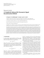
4.4. The Decision Function
4.4.1. Bipolar Decision Function. When BPSK modulation
is used, only two signal levels are required to transmit
information. Therefore, since only two signal levels are used,
a bipolar decision function is used in the HNN BPSK
MLSE equalizer. This function, also called a bipolar sigmoid
function, is expressed as
g
(
u
)
=

2
1+e
−u
− 1,
(21)
and is shown in Figure 3. It must also be noted that the
bipolar decision can also be used in the M-QAM model for
equalization in 4-QAM systems. This is an exception, since,
although 4-QAM modulation uses four signal levels, there
are only two signal levels per dimension. By using the model
derived for M-QAM modulation, 4-QAM equalization can
be performed by using the bipolar decision function in (21),
with the output scaled by ’n factor 1/
√
2.
4.4.2. Multile vel Decision Function. Apart from 4-QAM
modulation, all other M-QAM modulation schemes use
multiple amplitude levels to transmit information as the
“AM” in the acronym M-QAM implies. A bipolar decision
function will therefore not be sufficient; a multilevel decision
function with Q
= log
2
(M) distinct signal levels must be
used, where M is the modulation alphabet size.
A multilevel decision function can be realized by adding
several bipolar decision functions and shifting each by a
predetermined value, and scaling the result accordingly [29,
30]. To realize a Q-level decision function for use in an
−1

−0.8
−0.6
−0.4
−0.2
0
0.2
0.4
0.6
0.8
1
g(u)
−30 −20 −10 0 10 20 30
u
φ
= 10
φ
= 15
φ
= 20
Figure 4: The four-level decision function.
M-QAM HNN MLSE equalizer, the following function can
be used:
g
(
u
)
=
2
√
2

(
Q −1
)
⎛
⎝
(Q/2)−1

k=−((Q/2)−1)
1
1+e
−(u+φk)
⎞
⎠
−
1
√
2
,
(22)
where M is the modulation alphabet size and φ is the value by
which the respective bipolar decision functions are shifted.
Figure 4 shows the four-level decision function used for the
16-QAM HNN MLSE equalizer, for φ
= 10, φ = 15 and φ =
20.
Due to the time-varying nature of a mobile wireless com-
munication channel and energy losses caused by absorption
and scattering, the total power in the received signal is also
time-variant. This complicates equalization when using the
M-QAM HNN MLSE equalizer, since the value by which

the respective bipolar decision functions are shifted, φ,is
dependent on the power in the channel and will therefore
have a different value for every new data block arriving at the
receiver. For this reason the Q-level decision function in (22)
will change slightly for every data block. φ is determined by
the Euclidean norm of the estimated CIR and is given by
φ
=h=





⎛
⎝
L−1

k=0

h
(i)
k

2
⎞
⎠
2
+
⎛
⎝

L−1

k=0

h
(q)
k

2
⎞
⎠
2
,
(23)
where h
(i)
k
and h
(q)
k
are the kth respective in-phase and
quadrature components of the estimated CIR of length L as
before.
Figure 4 shows the four-level decision function for
different values of φ to demonstrate the effect of varying
power levels in the channel. Higher power in h will cause the
outer neurons to move away from the origin whereas lower
EURASIP Journal on Advances in Signal Processing 7
power will cause the outer neurons to move towards the
origin. Therefore, upon reception of a complete data block, φ

is determined according to the power of the CIR, after which
equalization commences.
4.5. Optimization. Because MLSE is an NP-complete prob-
lem, there are a number of possible “good” solutions in
the multidimensional solution space. By enumerating every
possible solution, it will be possible to find the best solution,
that is, the sequence of symbols that minimizes (4)and(5),
but it is not computationally feasible for systems with large
N and L. The HNN is used to minimize (5)tofindanear-
optimal solution at very low computational cost. Because
the HNN usually gets stuck in suboptimal local minima, it
is necessary to employ optimization techniques as suggested
[31]. To aid the HNN in escaping less optimal basins of
attraction simulated annealing and asynchronous neuron
updates are often used.
Markov Chain Monte Carlo (MCMC) algorithms are
used together with Gibbs sampling in [32]toaidopti-
mization in the solution space. According to [32], however,
the complexity of the MCMC algorithms may become
prohibitive due to the so called stalling problem, which
result from low probability transitions in the Gibbs sampler.
To remedy this problem an optimization variable referred
to as the “temperature” can be adjusted in order to avoid
these small transition probabilities. This idea is similar to
simulated annealing, where the temperature is adjusted to
control the rate of convergence of the algorithm as well as
the quality of the solution it produces.
4.5.1. Simulated Annealing. Simulated annealing has its
origin in metallurgy. In metallurgy annealing is the process
used to temper steel and glass by heating them to a high

temperature and then gradually cooling them, thus allowing
the material to coalesce into a low-energy crystalline state
[28]. In neural networks, this process is imitated to ensure
that the neural network escapes less optimal local minima to
converge to a near-optimal solution in the solution space. As
the neural network starts to iterate, there are many candidate
solutions in the solution space, but because the neural
network starts to iterate at a high temperature, it is able to
escape the less optimal local minima in the solutions space.
As the temperature decreases, the network can still escape less
optimal local minima, but it will start to gradually converge
to the global minimum in the solution space to minimize
the energy. This state of minimum energy corresponds to the
optimal solution.
The output of the function β(
·)in(20)isusedfor
simulated annealing. As the system iterates, n is incremented
with each iteration, and β(
·) produces a value according to
an exponential function to ensure that the system converges
to a near-optimal local minimum in the solution space. This
function is give by
β
(
n
− 1
)
= 5
2(n−Z+1)/Z
,

(24)
and shown in Figure 5. This causes the output of β(
·) to start
at a near-zero value and to exponentially converge to 1 with
each iteration.
0
0.1
0.2
0.3
0.4
0.5
0.6
0.7
0.8
0.9
1
2 4 6 8 10 12 14 16 18 20
Iteration number (n)
Figure 5: β-updates for Z = 20 iterations.
−1
−0.8
−0.6
−0.4
−0.2
0
0.2
0.4
0.6
0.8
1

g(u)
−30 −20 −10 0 10 20 30
u
β
= 1
β
 1
Figure 6: Simulated annealing on the bipolar decision function for
Z
= 20 iterations.
The effect of annealing on the bipolar and four-level
decision function during the iteration cycle is shown in
Figures 6 and 7, respectively, with the slope of the decision
function increasing as β(
·)isupdatedwitheachiteration.
Simulated annealing ensures near-optimal sequence estima-
tion by allowing the system to escape less optimal local
minima in the solution space, leading to better system
performance.
Figures 8 and 9 show the neuron outputs, for the real and
complex symbol components, of the 16-QAM HNN MLSE
equalizer for each iteration of the system with and without
annealing. It is clear that annealing allows the outputs of the
neuronstograduallyevolveinordertoconvergetonear-
optimal values in the N-dimensional solution space, not
produce reliable transmitted symbol estimates.
8 EURASIP Journal on Advances in Signal Processing
−1
−0.8
−0.6

−0.4
−0.2
0
0.2
0.4
0.6
0.8
1
g(u)
−30 −20 −10 0 10 20 30
u
β
= 1
β
 1
Figure 7: Simulated annealing on the four-level decision function
for Z
= 20 iterations.
−0.6
−0.4
−0.2
0
0.2
0.4
0.6
Neuron output
123456789101112
Iteration number (n)
Figure 8: Convergence of the 16-QAM HNN MLSE equalizer
without annealing.

4.5.2. Asynchronous Updates. In artificial neural networks,
the neurons in the network can either be updated using
parallel or asynchronous updates. Consider the iterative
solution of the HNN in (20). Assume that u, s and I each
contain N elements and that T is an N
× N matrix with Z
iterations as before.
When parallel neuron updates are used, N elements in
u
(n)
are calculated before N elements in s
(n)
are determined,
for each iteration. This implies that the output of the
neurons will only be a function of the neuron outputs
from the previous iteration. On the other hand, when
using asynchronous neuron updates, one element in s
(n)
is
determined for every corresponding element in u
(n)
. This
is performed N times per iteration—once for each neuron.
Asynchronous updates allow the changes of the neuron
outputs to propagate to the other neurons immediately
[31], while the output of all of the N neurons will only be
propagated to the other neurons after all of them have been
updated when parallel updates are used.
With parallel updates the effect of the updates propagates
through the network only after one complete iteration cycle.

This implies that the energy of the network might change
−0.6
−0.4
−0.2
0
0.2
0.4
0.6
Neuron output
2 4 6 8 10 12 14 16 18 20
Iteration number (n)
Figure 9: Convergence of the 16-QAM HNN MLSE equalizer with
annealing.
drastically, because all of the neurons are updated together.
This will cause the state of the neural network to “jump”
around on the solution space, due to the abrupt changes in
the internal state of the network. This will lead to degraded
performance, since the network is not allowed to gradually
evolve towards an optimal, or at least a near-optimal, basin
of attraction.
With asynchronous updates the state of the network
changes after each element in u
(n)
is determined. This
means that the state of the network undergoes N gradual
changes during each iteration. This ensures that the network
traverses the solution space using small steps while searching
for the global minimum. The computational complexity is
identical for both parallel and asynchronous updates [31].
Asynchronous updates are therefore used for the HNN MLSE

equalizer. The neurons are updated in a sequential order:
1, 2, 3, , N.
4.6. Convergence and Performance. Therateofconvergence
and the performance of the HNN MLSE equalizer are
dependent on the number of CIR coefficients L as well
as the number of iterations Z. Firstly, the number of CIR
coefficients determines the level of interconnection between
the neurons in the network. A long CIR will lead to dense
population of the connection matrix in X (10), consisting
of X
i
in (11)andX
q
(12), which translates to a high level
of interconnection between the neurons in the network. This
will enable the HNN MLSE equalizer to converge faster while
producing better maximum likelihood sequence estimates,
which is ultimately the result of a high level of diversity
provided by a highly dispersive channel. Similarly, a short
CIR will result in a sparse connection matrix X, where the
HNN MLSE equalizer will converge slower while yielding less
optimal maximum likelihood sequence estimates.
Second, simulated annealing, which allows the neuron
outputs to be forced to discrete decision levels when the
iteration number reaches the end of the iteration cycle (when
n
= Z), ensures that the HNN MLSE equalizer will have
converged by the last iteration (as dictated by Z). This is
clear from Figure 9. For small Z, the output of the HNN
MLSE equalizer will be less optimal than for large Z.Itwas

found that the HNN MLSE equalizer produces acceptable
performance without excessive computational complexity
for Z
= 20.
EURASIP Journal on Advances in Signal Processing 9
4.7. Soft Outputs. To enable the HNN MLSE equalizer to
produce soft outputs, β(
·)in(24) is scaled by a factor 0.5.
This allows the outputs of the equalizer to settle between the
discrete decision levels instead of being forced to settle on the
decision levels.
5. Computational Complexity Analysis
The computational complexity of the HNN MLSE equalizer
is quadratic in the data block length N and approximately
independent of the CIR length L for practical systems
where the data block length is larger than channel memory
length. This is due to the high parallelism of its underlying
neural network structure an high level of interconnection
between the neurons. The approximate independence of the
complexity from the channel memory is significant, as the
CIR length is the dominant term in the complexity of all
optimal equalizers, where the complexity is O(NM
L−1
).
In this section, the computational complexity of the
HNN MLSE equalizer is analyzed, where it is compared
to that of the Viterbi MLSE equalizer. The computational
complexities of these algorithms are analyzed by assuming
that an addition as well as a multiplication are performed
using one machine instruction. It is also assumed that

variable initialization does not add to the cost.
5.1. HNN MLSE Equalizer. The M-QAM HNN MLSE
equalizer performs the following steps. (The computational
complexity of the BPSK HNN MLSE equalizer is easily
derived from that of the M-QAM HNN MLSE equalizer.)
(1) Determine α and γ values using the est imated CIR:
There are L
− 1 distinct α values and L − 1 distinct γ values.
α
1
and γ
1
both contain L − 1 terms, each consisting of a
multiplication between two values. Also, α
L−1
and γ
L−1
both
contain one term. Therefore the number of computations to
determine all α-andγ values can be written as
2
L−1

n=1
n +2
L−1

n=1
n = 4
L−1


n=1
n
= 4
(
1+2+···+
(
L − 1
))
= 4
(((
L − 1
)
+1
)
+
((
L − 2
)
+2
)
+
((
L
− 3
)
+3
)
+
((

L −
(
L+1
))
+
(
L +1
)))
= 4
(
L − 1
)

L − 1
2

=
2
(
L − 1
)
2
.
(25)
(2) Populate matrices T
i
and T
q
(of size N ×N)andvectors
I

i
and I
q
(of size N). Under the assumption that variable
initialization does not add to the total cost, the population of
T
i
and T
q
does not add to the cost. However, I
i
and I
q
are not
only populated, but some calculations are performed before
population. All elements in I
i
and I
q
need L additions of two
multiplicative terms. Also, the first and the last L
−1 elements
in I
i
and I
q
together contain (L −1)
2
α and γ addition and/or
subtraction terms. Therefore, the cost of populating I

i
and I
q
is given by
2N

n=1
L
−1

m=1
m +4
(
L − 1
)
2
= 2N
(
L − 1
)
+4
(
L − 1
)
2
.
(26)
(3) Initialize s
= [s
T

i
| s
T
q
] and u = [u
T
i
| u
T
q
],bothof
length 2N. Under the assumption that variable initialization
does not add to the total cost, initialization of these variables
does not add to the cost.
(4) Iterate the system Z times:
(i) Determinethestatevector[u
T
i
| u
T
q
]
(n)
=

X
i
X
T
q

X
q
X
i

[s
i
/s
q
]
(n−1)
+[I
T
i
| I
T
q
]. The cost of multiply-
ing a matrix of size 2N
× 2N with a vector of size 2N
and adding another vector of length 2N to the result,
Z times, is given by
Z
⎛
⎝
2N

n=1
⎛
⎝

2N

m=1
m
⎞
⎠
+2N
⎞
⎠
=
Z

(
2N
)
2
+2N

=
(
2N
)
2
Z +2ZN.
(27)
(ii) Calculate [s
T
i
| s
T

q
]
(n)
= g(β(n)[u
T
i
| u
T
q
]
(n−1)
)Z
times. The cost of calculating the estimation vector
s of length 2N by using every value in state vector u,
also of length 2N, assuming that the sigmoid function
uses three instructions to execute, Z times, is given
by (it is assumed that the values of β(n)isstoredina
lookup table, where n
= 1, 2,3, , Z, to trivialize the
computational complexity of simulated annealing)
3
× 2ZN = 6ZN.
(28)
Thus, by adding all of the computations above, the total
computational complexity for the M-QAM HNN MLSE
equalizer is
(
2N
)
2

Z +8ZN +2N
(
L − 1
)
+6
(
L − 1
)
2
.
(29)
The structure of the M-QAM HNN MLSE equalizer is
identical to that of the BPSK HNN MLSE equalizer. The
only difference is that, for the BPSK HNN MLSE equalizer,
all matrices and vectors are of dimension N and instead
of 2N, as only the in-phase component of the estimated
symbol vector is considered. Therefore, it follows that
the computational complexity of the BPSK HNN MLSE
equalizer will be
N
2
Z +4ZN + N
(
L − 1
)
+3
(
L − 1
)
2

.
(30)
5.2. Viterbi MLSE Equalizer. The Viterbi equalizer performs
the following steps:
(1) Setup trellis of length N, where each stage contains
M
L−1
states, where M is the constellation size: It is
assumed that this does not add to the complexity. It
must however be noted that the dimensions of the
trellis is N
× M
L−1
.
10 EURASIP Journal on Advances in Signal Processing
(2) Determine two Euclidean distances for each node.The
Euclidean distance is determined by subtracting L
addition terms, each containing one multiplication,
from the received symbol at instant k. The cost for
determining one Euclidean distance is therefore given
by
2NM
L−1
(
2L +1
)
= 4LNM
L−1
+2NM
L−1

.
(31)
(3) Eliminate contending paths at each node.Twopath
costs are compared using an if -statement, assumed
to count one instruction. The cost is therefore
2NM
L−1
.
(32)
(4) Backtrack the trellis to determine the MLSE solution.
Backtracking accross the trellis, where each time
instant k requires an if -statement. The cost is there-
fore
NM
L−1
.
(33)
Adding all costs to give the total cost results in
4LNM
L−1
+5NM
L−1
.
(34)
5.3. HNN MLSE Equalizer and Viterbi MLSE Equalizer Com-
parison. Figure 10 shows the computational complexities of
the HNN MLSE equalizer and the Viterbi MLSE equalizer as
a function of the CIR length L,forL
= 2toL = 10, where
the number of iterations is Z

= 20. For the HNN MLSE
equalizer, it is shown for BPSK and M-QAM modulation,
since the computational complexities of all M-QAM HNN
MLSE equalizers are equal. Also, for the Viterbi MLSE
equalizer, it is shown for BPSK and 4-QAM modulation. It is
clear that the computational complexity of the HNN MLSE
equalizer is superior to that of the Viterbi MLSE equalizer for
system with larger memory. For BPSK, the break-even mark
between the HNN MLSE equalizer and the Viterbi MLSE
equalizer is at L
= 7, and for 4-QAM it is at L = 4.2 ≈ 4.
The complexity of the HNN MLSE equalizer for both
BPSK and M-QAM seems constant whereas that of the
Viterbi MLSE equalizer increases exponentially as the CIR
length increases. Also, note the difference in complexity
between the BPSK HNN MLSE equalizer and the M-
QAM HNN MLSE equalizer. This is due to the quadratic
relationship between the complexity and the data block
length, which dictates the size of the vectors and matrices
in the HNN MLSE equalizer. The HNN MLSE equalizer is
however not well-suited for systems with short CIRs, as the
complexity of the Viterbi MLSE equalizer is less than that of
the HNN MLSE equalizer for short CIRs. This is however
not a concern, since the aim of the proposed equalizer is
on equalization of signals in systems with extremely long
memory.
Figure 11 shows the computational complexity of the
HNN MLSE equalizer for BPSK and M-QAM modulation
for block lengths of N
= 100 and N = 500, respectively,

indicating the quadratic relationship between the computa-
tional complexity and the data block length, also requiring
0
1
2
3
4
5
6
7
8
9
10
×10
5
Number of computations
2345678910
CIR length (L)
BPSK HNN MLSE
M-QAM HNN MLSE
BPSK Viterbi MLSE
4-QAM Viterbi MLSE
Figure 10: Computational complexity comparison between the
HNN MLSE and Viterib MLSE equalizers.
larger vectors and matrices in the HNN MLSE equalizer. It is
clear that, as the data block length increases, the data block
length N, rather than the CIR length L, is the dominant factor
contributing to the computational complexity. However, due
to the approximate independence of the complexity on the
CIR length, the HNN MLSE equalizer is able to equalize

signals in systems with hundreds of CIR elements for large
data block lengths. This should be clear from Figures 10 and
11.
The scenario in Figure 11 is somewhat unrealistic, since
the data block length must at least be as long as the CIR
length. However, Figure 12 serves to show the effect of the
data block length and the CIR length on the computational
complexity of the HNN MLSE equalizer. Figure 12 shows the
computational complexity for a more realistic scenario. Here
the complexity of the BPSK HNN MLSE and the M-QAM
HNN MLSE equalizer is shown for N
= 1000, N = 1500 and
N
= 2000, for L = 0toL = 1000.
From Figure 12 it is clear that the computational com-
plexity increases quadratically as the data block length
linearly increases. It is quite significant that the complexity
is nearly independent of the CIR length when the data block
length is equal to or great then the CIR length, which is the
case in practical communication systems. It should now be
clear why the HNN MLSE equalizer is able to equalize signals
in systems, employing BPSK or M-QAM modulation, with
hundreds and possibly thousands of resolvable multipath
elements.
The superior computational complexity of the HNN
MLSE equalizer is obvious. Its low complexity makes it
suitable for equalization of signals with CIR lengths that
are beyond the capabilities of optimal equalizers like the
Viterbi MLSE equalizer and the MAP equalizer, for which
EURASIP Journal on Advances in Signal Processing 11

0
0.5
1
1.5
2
2.5
3
×10
7
Number of computations
0 100 200 300 400 500 600 700 800 900 1000
CIR length (L)
BPSK HNN MLSE: N
= 100
M-QAM HNN MLSE: N
= 100
BPSK HNN MLSE: N
= 500
M-QAM HNN MLSE: N
= 500
Figure 11: Computational complexity comparison for the HNN
MLSE equalizers for different data block lengths.
the computational complexity increases exponentially with
an increase in the channel memory (note that the computa-
tional complexity graphs of the Viterbi MLSE equalizer can-
not be presented on the same scale as that of the HNN MLSE
equalizer, as shown in Figure 10 through Figure 12), and it
is also exponentially related to the number of symbols in the
modulation alphabet. On the other hand, the computational
complexity of the HNN MLSE equalizer is quadratically

related to the data block length and almost independent of
the CIR length for realistic scenarios. Also, the complexity of
the HNN MLSE equalizer is independent of the modulation
alphabet size for M-QAM systems, making it suitable for
equalization in higher order M-QAM system with even
moderate channel memory, where optimal equalizer cannot
be applied.
6. Simulation Results
In this section, the HNN MLSE equalizer is evaluated. The
low computational complexity of the HNN MLSE equalizer
allows it to equalize signals in systems with extremely
long memory, well beyond the capabilities of conventional
optimal equalizers like the Viterbi MLSE and the MAP
equalizers. The HNN MLSE equalizer is evaluated for
long sparse and dense Rayleigh fading channels. It will be
established that the HNN MLSE equalizer outperforms the
MMSE equalizer in long fading channels and it will be shown
that the performance of the HNN MLSE equalizer in sparse
channels is better than its performance in equivalent dense
channels, that is, longer channels with the same amount of
nonzero CIR taps.
0
0.5
1
1.5
2
2.5
3
3.5
×10

8
Number of computations
0 100 200 300 400 500 600 700 800 900 1000
CIR length (L)
BPSK HNN MLSE: N
= 1000
M-QAM HNN MLSE: N
= 1000
BPSK HNN MLSE: N
= 1500
M-QAM HNN MLSE: N
= 1500
BPSK HNN MLSE: N
= 2000
M-QAM HNN MLSE: N
= 2000
Figure 12: Computational complexity comparison for the HNN
MLSE equalizers for realistic data block lengths.
The communication system is simulated for a GSM
mobile fading environment, where the carrier frequency is
f
c
= 900 MHz, the symbol period is T
s
= 3.7 μsand
the relative speed between the transmitter and receiver is
v
= 3 km/h. To simulate the fading effect on each tap,
the Rayleigh fading simulator proposed in [33] is used to
generate uncorrelated fading vectors. Least Squares (LS)

channel estimation is used to determine an estimate for the
CIR, in order to include the effect of imperfect channel
state information (CSI) in the simulation results. Where
perfect CSI is assumed, however, the statistical average of
each fading vector is used to construct the CIR vector for
each received data block. In all simulations, the nominal CIR
weights are chosen as h
={h
0
/h, h
1
/h, , h
L−1
/h}
such that h
T
h = 1, where L is the CIR length, and h
is a column vector of length L, in order to normalize the
energy in the channel. The normalized nominal taps are
used to scale the uncorrelated fading vectors produced by the
Rayleigh fading simulator. To simulated dense channels, all
the nominal tap weights are chosen as 1, after which the taps
are normalized as explained. To simulated sparse channels,
K% of the nominal taps weights are chosen as 1 (for sparse
channels the nonzero taps are evenly spaced), while the rest
are set to zero. Again the taps are normalized, but now only
K%ofL taps are nonzero.
In order to compare the performance of the HNN MLSE
equalizer in dense channels to its performance in sparse
channels, an equivalent dense channel is used. An equivalent

dense channel is a dense channel with an equal amount
of nonzero taps as that of a sparse channel of any length.
12 EURASIP Journal on Advances in Signal Processing
0
0.5
1
We ig h t
0 20 40 60 80 100
Nominal CIR tap
(a)
0
0.5
1
We ig h t
0 20 40 60 80 100
Nominal CIR tap
(b)
0
0.5
1
We ig h t
0 20 40 60 80 100
Nominal CIR tap
(c)
0
0.5
1
We ig h t
0 20 40 60 80 100
Nominal CIR tap

(d)
Figure 13: Normalized evenly spaced nominal CIR taps of sparse channels. (a) K = 100% (b) K = 50% (c) K = 25% (d) K = 10%.
A sparse channel of length L,whereonlyK% of the taps
are nonzero, is compared to a dense channel of length [L
·
K]/100, so that the number of nonzero taps in the sparse
channel is equal to that in the equivalent dense channel.
Figure 13 shows the evenly spaced normalized nominal CIR
taps of sparse channels of length L
= 100, where K = 100%
(a), K
= 50% (b), K = 25% (c) and K = 10% (d), reducing
the number of nonzero CIR taps to K% of the CIR length.
6.1. Performance in Dense Channels. The performance of
the BPSK HNN MLSE equalizer and 16-QAM HNN MLSE
equalizers is evaluated for long dense channels, for perfect
CSI, with channel delays from 74 μsto1.9ms(L
= 10 to L =
500). The performance of the BPSK HNN MLSE equalizer is
also compared to that of an MMSE equalizer for imperfect
CSI.
Figure 14 shows the performance of the BPSK HNN
MLSE equalizer for perfect CSI, where the uncoded data
block length is N
= 500 and the CIR lengths range from
L
= 10 to L = 500, corresponding to channel delay spreads of
37 μsto1.85 ms. As the channel memory increases, the per-
formance increases correspondingly, approaching unfaded
matched filter performance as a result of the effective time

diversity provided by the multipath channels. It is clear the
BSPK HNN MLSE equalizer performs near-optimal, if not
optimal, equalization. Note that for L
= 500, a Viterbi MLSE
equalizer would require M
L−1
= 2
499
states in its trellis per
transmitted symbol.
Figure 15 shows the performance of the 16-QAM HNN
MLSE equalizer, where again perfect CSI and an uncoded
data block length of N
= 500 are assumed. Here, the CIR
length ranges from L
= 25 to L = 400 which corresponds
tochanneldelayspreadsof92.5 μsto1.48 ms. Here, it is
also clear that the performance approaches unfaded matched
filter performance as the channel memory increases. Note
that a Viterbi MLSE equalizer would require M
L−1
= 16
399
states in its trellis per transmitted symbol for L = 400.
10
−6
10
−5
10
−4

10
−3
10
−2
10
−1
BER
02468101214
E
b
/N
0
(dB)
HNN MLSE: L
= 10
HNN MLSE: L
= 20
HNN MLSE: L
= 50
HNN MLSE: L
= 100
HNN MLSE: L
= 200
HNN MLSE: L
= 500
BPSK bound
Rayleigh diversity order 1
Figure 14: BPSK HNN MLSE equalizer performance in extremely
long channels.
Figure 16 shows the performance of the BPSK HNN

MLSE equalizer compared to that of an MMSE equalizer,
for moderate to long channels, using channel estimation.
It is assumed that 3L training symbols are available for
channel estimation per data block of length N
= 450.
For the HNN MLSE equalizer the LS channel estimator is
used to estimate the CIR using 3L training symbols, and
for the MMSE equalizer the channel is estimated as part
of the filter coefficient optimization—an integral part of
MMSE equalization—where the filter smoothing length is
EURASIP Journal on Advances in Signal Processing 13
10
−8
10
−7
10
−6
10
−5
10
−4
10
−3
10
−2
10
−1
10
0
BER

0 2 4 6 8 10121416
E
b
/N
0
(dB)
HNN MLSE: L
= 25
HNN MLSE: L
= 50
HNN MLSE: L
= 100
HNN MLSE: L
= 250
HNN MLSE: L
= 400
16-QAM bound
Rayleigh diversity order 1
Figure 15: 16-QAM HNN MLSE equalizer performance in
extremely long channels.
3L.FromFigure 16 it is clear that the HNN MLSE equalizer
outperforms the MMSE equalizer for high E
b
/N
0
-levels and
when the channel memory is large.
From these results it is clear that the HNN MLSE equal-
izer effectively equalizes the received signal and performs
near-optimally when the channel memory is large, if perfect

CSIisassumed.
6.2. Performance in Sparse Channels. The performance of
the BSPK HNN MLSE equalizer, and 16-QAM HNN MLSE
equalizers is evaluated for sparse channels, where their
performance is compared to equivalent dense channels. The
equalizer is simulated for various levels op sparsity, where
K indicates the percentage of nonzero CIR taps. The perfor-
mance of the HNN MLSE equalizers in these sparse channels
is compared to their performance in equivalent dense
channels of length L
= 10 to L = 100. Perfect CSI is assumed.
For the BPSK HNN MLSE equalizer an uncoded data
block length of N
= 200 is used where the channel delay of
the sparse channel is 0.74 ms, corresponding to a CIR length
of L
= 100. To simulate the BPSK equalizer K is chosen as
K
= 10%, K = 20%, K = 40%, K = 60%, and K = 80%,
such that the number of nonzero taps in the CIR is 10, 20, 40,
60, and 80, respectively. Figure 17 shows the performance of
the BPSK HNN MLSE equalizer in a sparse channel of length
L
= 100, compared to its performance in dense channels of
length L
= 10 to L = 100. It is clear from Figure 17 that the
performance of the BPSK HNN MLSE equalizer in sparse
is better compared to the corresponding equivalent dense
channels. Because of the approximate independence of the
computational complexity on the CIR length, the increase in

complexity due to larger L is negligible.
10
−8
10
−7
10
−6
10
−5
10
−4
10
−3
10
−2
10
−1
BER
0 2 4 6 8 101214161820
E
b
/N
0
(dB)
HNN MLSE: L
= 6
HNN MLSE: L
= 10
HNN MLSE: L
= 20

HNN MLSE: L
= 40
HNN MLSE: L
= 60
HNN MLSE: L
= 80
MMSE: L
= 6
MMSE: L
= 10
MMSE: L
= 20
MMSE: L
= 40
MMSE: L
= 60
MMSE: L
= 80
Coded BPSK bound
Figure 16: BPSK HNN MLSE and MMSE equalizer performance
comparison.
The 16-QAM HNN MLSE equalizer is also simulated for
sparse channels, where the uncoded block length is N
= 200
and the channel delay spread is L
= 100 which corresponds
to 1.5 ms. Here, K is chosen as K
= 25% and K = 40%
such that the number of nonzero taps in the CIR is 25 and
40, respectively. Figure 18 shows the performance of the 16-

QAM HNN MLSE equalizer in a sparse channel of length
L
= 100, compared to its performance in dense channels
of length L
= 25 to L = 100. Here, again it is clear that
the performance of the equalizer in sparse channels is better
than its performance in the corresponding equivalent dense
channels. Again, the complexity increase for equalization in
sparse channels is negligible.
From the simulation results in Figures 17 and 18 it is
clear that the HNN MLSE equalizer performs well in sparse
channels compared to its performance in equivalent dense
channels. Having an equal amount of nonzero nominal CIR
taps, the performance increase in the sparse channels is not
attributed to more diversity due to extra multipath, but
rather to the higher level of interconnection between the
neurons in the HNN. (Longer estimated CIRs will allow the
connection matrix of the HNN to be more densely pop-
ulated, increasing the level of interconnection between the
neurons.) This allows the HNN MLSE equalizer to mitigate
the effect of multipath more effectively to produce better
performance in sparse channels than in their corresponding
equivalent dense channels.
Figure 19 shows the performance of the BPSK HNN
MLSE equalizer for various sparse channels, all with a fixed
amount of nonzero nominal CIR taps such that the level
14 EURASIP Journal on Advances in Signal Processing
10
−7
10

−6
10
−5
10
−4
10
−3
10
−2
10
−1
BER
2 3 4 5 6 7 8 9 10 11 12
E
b
/N
0
(dB)
HNN MLSE: L
= 100 (K = 10%)
HNN MLSE: L
= 100 (K = 20%)
HNN MLSE: L
= 100 (K = 40%)
HNN MLSE: L
= 10
HNN MLSE: L
= 20
HNN MLSE: L
= 40

HNN MLSE: L
= 100
BPSK bound
Rayleigh diversity order 1
Figure 17: BPSK HNN MLSE equalizer performance in sparse
channels.
10
−6
10
−5
10
−4
10
−3
10
−2
10
−1
BER
6 7 8 9 10 11 12 13 14
E
b
/N
0
(dB)
HNN MLSE: L
= 100 (K = 25%)
HNN MLSE: L
= 100 (K = 40%)
HNN MLSE: L

= 25
HNN MLSE: L
= 40
HNN MLSE: L
= 100
16-QAM bound
Rayleigh diversity order 1
Figure 18: 16-QAM HNN MLSE equalizer performance in sparse
channels.
10
−4
10
−3
10
−2
10
−1
BER
012345678910
E
b
/N
0
(dB)
HNN MLSE: L
= 20 (K = 100%)
HNN MLSE: L
= 60 (K = 33%)
HNN MLSE: L
= 100 (K = 20%)

HNN MLSE: L
= 140 (K = 14%)
BPSK bound
Rayleigh diversity order 1
Figure 19: BPSK HNN MLSE performance in sparse channels with
constant diversity.
10
−6
10
−5
10
−4
10
−3
10
−2
10
−1
BER
6 7 8 9 10 11 12 13 14
E
b
/N
0
(dB)
HNN MLSE: L
= 50 (K = 100%)
HNN MLSE: L
= 100 (K = 50%)
HNN MLSE: L

= 200 (K = 25%)
HNN MLSE: L
= 300 (K = 16.7%)
16-QAM bound
Rayleigh diversity order 1
Figure 20: 16-QAM HNN MLSE performance in sparse channels
with constant diversity.
EURASIP Journal on Advances in Signal Processing 15
of diversity due to multipath remains constant. Using an
uncoded data block length of N
= 200 and with L such
that [L
· K]/100 = 20 for K = 100%, K = 33%, K =
20% and K = 14% (corresponding to L = 20, L = 60,
L
= 100 and L = 140), it is clear that the performance
increases as the CIR length L increases, although the number
of multipath channels remains unchanged for all cases. Also,
Figure 20 shows the performance of the 16-QAM HNN
MLSE equalizer. Using an uncoded data block length of N
=
400 and with L such that [L · K]/100 = 50 for K = 100%,
K
= 50%, K = 25% and K = 16.7% (corresponding to
L
= 50, L = 100, L = 200 and L = 300), the performance
increases with an increase in L.
From these results in is clear that the BER performance
increases with an increase in L. The HNN MLSE equalizer
thus exploits sparsity in communication channels by reduc-

ing the BER as the level of sparsity increases, given that the
nonzero CIR taps remains constant.
7. Conclusion
In this paper, a low complexity MLSE equalizer was proposed
for use in single-carrier M-QAM modulated systems with
extremely long memory. The equalizer has computational
complexity quadratic in the data block length and approx-
imately independent of the channel memory length. An
extensive computational complexity analysis was performed,
and the superior computational complexity of the proposed
equalizer was graphically presented. The HNN was used as
the basis of this equalizer due to its low complexity opti-
mization ability. It was also highlighted that the complexity
of the equalizer for any single carrier M-QAM system is
independent of the number of symbols in the modulation
alphabet, allowing for equalization in 256-QAM systems
with equal computational cost as for 4-QAM systems, which
is not possible with conventional optimal equalizers like the
VA and MAP.
When the equalizer was evaluated for extremely long
channels for perfect CSI its performance matched unfaded
AWGN performance, providing enough evidence to assume
that the equalizer performs optimally for extremely long
channels. It is therefore assumed that the performance of
the equalizer approaches optimality as the connection matrix
of the HNN is populated. It was also shown that the HNN
MLSE equalizer outperforms an MMSE equalizer at high
E
b
/N

0
values.
The HNN MLSE equalizer was evaluated for sparse
channels and it was shown that its performance was better
compared to its performance in equivalent dense channels,
with a negligible increase in computational complexity. It
was also shown how the equalizer exploits channel sparsity.
The HNN MLSE equalizer is therefore very attractive for
equalization in sparse channels, due to its low complexity and
good performance.
With its low complexity equalization ability, the HNN
MLSE equalizer can find application in systems with
extremely long memory lengths, where conventional optimal
equalizers cannot be applied.
References
[1] G. D. Forney Jr., “Maximum likelihood sequence estimation of
digital sequences in the presence of intersymbol interference,”
IEEE Transactions on Information Theor y,vol.18,no.3,pp.
363–378, 1972.
[2] A. D. Viterbi, “Error bounds for convolutional codes and an
asymptotically optimum decoding algorithm,” IEEE Transac-
tions on Information Theory, vol. 13, no. 1, pp. 260–269, 1967.
[3] L. R. Bahl, J. Cocke, F. Jelinek, and J. Raviv, “Optimal decoding
of linear codes for minimizing symbol error rate,” IEEE
Transactions on Information Theory, vol. 20, no. 2, pp. 284–
287, 1974.
[4]J.G.Proakis,Digital Communications, McGraw-Hill, New
York, NY, USA, 4th edition, 2001.
[5] A. Duel-Hallen and C. Heegard, “Delayed decision-feedback
sequence estimation,” IEEE Transactions on Communications,

vol. 37, no. 5, pp. 428–436, 1989.
[6] W. U. Lee and F. S. Hill Jr., “A maximum likelihood sequence
estimator with decision feedback equalizer,” IEEE Transactions
on Communications, vol. 25, no. 9, pp. 971–979, 1977.
[7] W. H. Gerstacker and R. Schober, “Equalization concepts for
EDGE,” IEEE Transactions on Wireless Communications, vol. 1,
no. 1, pp. 190–199, 2002.
[8] A. Goldsmith, Wireless Communications, Cambridge Univer-
sity Press, Cambridge, UK, 2005.
[9] J. Terry and J. Heiskala, OFDM Wireless LANs: A Theoretical
and Practical Guide, Sams, Indianapolis, Ind, USA, 2001.
[10] R. R. Lopes and J. R. Barry, “The soft-feedback equalizer
for turbo equalization of highly dispersive channels,” IEEE
Transactions on Communications, vol. 54, no. 5, pp. 783–788,
2006.
[11] M. Stojanovic, L. Freitag, and M. Johnson, “Channel-
estimation-based adaptive equalization of underwater acous-
tic signals,” Oceans, vol. 2, pp. 985–990, 1999.
[12] M. Zimmermann and K. Dostert, “A multipath model for the
powerline channel,” IEEE Transactions on Communications,
vol. 50, no. 4, pp. 553–559, 2002.
[13] J. W. M. Bergmans, Digital Baseband Transmission and
Recording, Springer, New York, NY, USA, 1996.
[14] H. C. Myburgh and J. C. Olivier, “Low complexity iterative
MLSE equalization of M-QAM signals in extremely long
rayliegh fading channels,” in Proceedings of the European
International Science Fiction Convention (EUROCON ’09),pp.
1632–1637, 2009.
[15] J. J. Hopfield and D. W. Tank, “Neural computation of
decisions in optimization problems,” Biological Cybernetics,

vol. 52, no. 3, pp. 141–152, 1985.
[16] H. H. Zeng, L. Ye, and J. H. Winters, “Improved spatial-
temporal equalization for EDGE: a fast selective-direction
MMSE timing recovery algorithm and two-stage soft-output
equalizer,” IEEE Transactions on Communications, vol. 49, no.
12, pp. 2124–2134, 2001.
[17] X. Dayong, X. Yang, and D. Haifeng, “An improved algorithm
of MMSE multiuser detection for CDMA systems,” in Pro-
ceedings of the International Sy mposium on Communications
and Information Technologies (ISCIT ’05), vol. 1, pp. 552–555,
2005.
[18] H. Zhou and S. Zhou, “Improved adaptive MMSE detector for
downlink multi-cell MIMO signals,” in Proceedings of the 60th
IEEE Vehicular Technology Conference (VTC ’04), pp. 3733–
3737, September 2004.
[19] N. Czink, G. Matz, D. Seethaler, and F. Hlawatsch, “Improved
MMSE estimation of correlated MIMO channels using
16 EURASIP Journal on Advances in Signal Processing
a structured correlation estimator,” in Proceedings of the
IEEE Workshop on Signal Processing Advances in Wireless
Communications (SPAWC ’05), pp. 595–599, 2005.
[20] J H. Park, Y. Whang, and K. S. Kim, “Low complexity MMSE-
SIC equalizer employing time-domain recursion for OFDM
systems,” IEEE Signal Processing Letters, vol. 15, pp. 633–636,
2008.
[21] Z. Rong and L. Guangqiu, “Low complexity code multiplexed
pilot aided adaptive MMSE equalizerfor CDMA systems,”
in Proceedings of the International Conference on Wireless
Communications, Networking and Mobile Computing, pp. 1–4,
2008.

[22] S. H. Bang, B. J. Sheu, and R. C H. Chang, “Maximum
likelihood sequence estimation of communication signals
by a Hopfield neural network,” in Proceedings of the IEEE
International Conference on Neural Networks, vol. 5, pp. 3369–
3374, July 1994.
[23] S. H. Bang and B. J. Sheu, “A neural network for detection of
signals in communication,” IEEE Transactions on Circuits and
Systems I, vol. 43, no. 8, pp. 644–655, 1996.
[24] J. D. Provence, “Neural network implementation for an
adaptive maximum-likelihood receiver,” in Proceedings of the
IEEE International Symposium on Circuits and Systems, vol. 3,
pp. 2381–2385, June 1988.
[25] D. C. Chen, B. J. Sheu, and E. Y. Chou, “A neural network
communication equalizer with optimized solution capability,”
in Proceedings of the IEEE International Conference on Neural
Networks, vol. 4, pp. 1957–1962, June 1996.
[26] J. J. Hopfield, “Artificial neural networks,” IEEE Circuits and
Devices Magazine, vol. 4, no. 5, pp. 3–10, 1988.
[27] J. C. Olivier, “Essential Digital Communication Theory,”
ESF320 Lecture notes, 2007.
[28] S. Russell and P. Norvig, Artificial Intelligence: AModern
Approach, Prentice-Hall, Upper Saddle River, NJ, USA, 2nd
edition, 2003.
[29]S.H.Bang,O.T C.Chen,J.C F.Chang,andB.J.Sheu,
“Paralleled hardware annealing in multilevel Hopfield neural
networks for optimal solutions,” IEEE Transactions on Circuits
and Systems II, vol. 42, no. 1, pp. 46–49, 1995.
[30] S. H. Bang, B. J. Sheu, and J. C F. Chang, “Search of optimal
solutions in multi-level neural networks,” in Proceedings of the
IEEE International Symposium on Circuits and Systems (ISCAS

’94), vol. 6, pp. 423–426, June 1994.
[31] U. Halici, “Artificial Neural Networks,” EE 543 Lecture notes,
2004.
[32] B. Farhang-Boroujeny, H. Zhu, and Z. Shi, “Markov chain
Monte Carlo algorithms for CDMA and MIMO communica-
tion systems,” IEEE Transactions on Signal Processing, vol. 54,
no. 5, pp. 1896–1909, 2006.
[33] Y. R. Zheng and C. Xiao, “Improved models for the generation
of multiple uncorrelated Rayleigh fading waveforms,” IEEE
Communications Letters, vol. 6, no. 6, pp. 256–258, 2002.